Option Pricing under Multiscale Stochastic Volatility
Cristina Tessari∗1 and Caio Almeida†1
1EPGE-FGV
Ongoing Master’s Thesis
First Draft: November 30, 2015
Abstract
The stochastic volatility model proposed by Fouque, Papanicolaou, and Sircar
(2000) explores a fast and a slow time-scale fluctuation of the volatility process to end up with a parsimonious way of capturing the volatility smile implied by close to the money options. In this paper, we test three different models of these authors using options on the S&P 500. First, we use model independent statistical tools to demonstrate the presence of a short time-scale, on the order of days, and a long time-scale, on the order of months, in the S&P 500 volatility. Our analysis of market data shows that both time-scales are statistically significant. We also provide a calibration method using observed option prices as represented by the so-called term structure of implied volatility. The resulting approximation is still independent of the particular details of the volatility model and gives more flexibility in the parametrization of the implied volatility surface. In addition, to test the model’s ability to price options, we simulate options prices using four different specifications for the Data generating Process. As an illustration, we price an exotic option.
Keywords: Option pricing; Stochastic volatility; Mean-reversion.
∗[email protected]; Corresponding author.
1
Introduction
Asset return volatility is a central concept in finance, whether in asset pricing, portfolio selection, or risk management. Although many well-known theoretical models assumed constant volatility (seeMerton,1969;Black and Scholes,1973), sinceEngle(1982) seminal paper on ARCH models, the financial literature has widely acknowledge that volatility is time-varying, in a persistent fashion, and predictable (seeAndersen and Bollerslev,1997).
From the point of view of derivative pricing and hedging, continuous time stochastic volatility models, which can be seen as continuous time versions of ARCH-type models, have become popular in the last twenty years. The idea of using stochastic volatility models to describe the dynamics of an asset price comes from empirical evidence indicating that asset price dynamics is driven by processes with time-varying volatility. In fact, two phenomena are observed: (i) a non-flat implied volatility surface when the Black and Scholes (1973) model is used to interpret financial data, and (ii) skewness and kurtosis are present in the asset price probability density function deduced from empirical data. These phenomena stands in empirical contradiction to the consistent use of a classical Black-Scholes approach to pricing options and similar securities, as the Black–Scholes model fails to correctly describe the market behavior.
Stochastic volatility models relax the constant volatility assumption of the Black-Scholes model by allowing volatility to follow a random process. In this context, the market is incomplete because the volatility is not traded and the volatility risk cannot be fully hedged using the basic instruments (stocks and bonds). To preclude arbitrage, the market selects a unique risk neutral derivative pricing measure, from a family of possible measures. As a result, in contrast to the Black-Scholes model, the stochastic volatil-ity models are able to capture some of the well-known features of the implied volatilvolatil-ity surface, such as the volatility smile and skew.
The presence of volatility factors is well documented in the literature using underlying returns data (seeAlizadeh et al.,2002;Andersen and Bollerslev,1997;Chernov et al.,2003;
Engle and Patton,2001;Fouque et al.,2003b;Hillebrand,2005;LeBaron,2001;Gatheral,
2006, for instance). While some single-factor diffusion stochastic volatility models such as
Heston(1993) enjoy wide success, numerous empirical studies of real data have shown that the two-factor stochastic volatility models can produce the observed kurtosis, fat-tailed return distributions and long memory effect. For example,Alizadeh, Brandt, and Diebold
that two factors are necessary for log-linear models. These evidences, among others, have motivated the development of multiscale stochastic volatility models as an efficient way to capture the principle effects on derivative pricing and portfolio optimization of randomly varying volatility.
In this paper, motivated by both the popularity and appeal of stochastic volatility models and by the difficulty associated with their estimation, we compare the performance of three different specifications of theFouque, Papanicolaou, and Sircar(2000) stochastic volatility model for pricing European call options with the Black-Scholes model. We assume that the underlying asset evolves according to a geometric Brownian motion, as in the Black and Scholes (1973) model, but with stochastic volatility. We use S&P 500 data to demonstrate that the volatility of this index is driven by two diffusions: one fast mean-reverting and one svarying. In order to identify these scales, we analyze low-and high-frequency data using the empirical structure function, or variogram, of the log absolute returns. To retrieve the scale on the order of months, we use daily closing prices of the S&P 500 over several years. To extract the scale on the order of days, we follow
Fouque et al. (2003a) and use high-frequency, intraday data.
In their work, Fouque, Papanicolaou, and Sircar (2000) show that multiscale stochas-tic volatility models lead to a first-order approximation of derivatives prices and of the implied volatility surface. By using a combination of singular and regular perturbations to approximate prices when volatility is driven by short and long time scale factors, they derive a first-order approximation for European options prices and their induced implied volatilities. This first-order approximation is composed by the Black-Scholes price and the first-order correction only involves Greeks. In terms of implied volatility, this pertur-bation analysis translates into an affine approximation in the log-moneyness to maturity ratio (LMMR). This perturbation method allows a direct calibration using real data of the group market parameters, which are exactly those needed to price exotic contracts at this level of approximation. The advantage of this approach is that the resulting formula for the option price does not depend on the unobserved current value of the volatil-ity. However, calibration of this model requires information on near-the-money implied volatilities.
block-length selection of Politis and White (2004). The second goal, conditional on the market supporting evidence of a multiscale stochastic volatility process, is related to the calibration of the model using option data on the underlying. At this stage, we compare the observed prices with the corrected Black-Scholes prices by using three different first-order corrections: (i) a fast time scale correction; (ii) a slow time scale correction; and (iii) a multiscale (fast and slow) correction. Finally, the third goal of this paper is to simulate both the trajectories of these three different corrected prices based on the model of Fouque, Papanicolaou, and Sircar (2000) and the Black-Scholes prices, and compare the prices of exotic derivatives based on these simulated prices.
The rest of this paper proceeds as follows. In Section 2, we describe the class of multiscale stochastic volatility models that we will work with. In Section 2.3, we present the empirical structure function, or variogram, which is used as an estimator of the speed of mean reversion. In Section 2.4, we present the first-order approximation derived in
Fouque, Papanicolaou, and Sircar (2000), which is valid for any European-style option. Additionally, we present an explicit formula for the implied volatility surface induced by the option pricing approximation. In Section 3, we report the numerical results. In Section 4, we show how the corrected Black-Scholes prices can be used to price exotic options. Finally, Section 5 concludes.
2
A Model for the Stock Price Dynamics
2.1
The Model
Let (Ω,F,P,{Ft}t≥0) be a complete probability space with a filtration satisfying the usual conditions. We consider a family of stochastic volatility models (Xt, Yt, Zt), where
Xt is the underlying price, and Yt and Zt are two mean-reverting Ornstein–Uhlenbeck
(OU) processes. Under the physical probability measure P, our model can be written as the following system of stochastic differential equations (SDE):
dXt =µXtdt+f(Yt, Zt)XtdWt0,
dYt = 1ǫα(Yt)dt+ √1ǫβ(Yt)dWt1,
dZt =δc(Zt)dt+ √
δg(Zt)dWt2,
(1)
where (W(0), W(1), W(2)) are correlated P-Brownian motions with
and |ρ1| < 1, |ρ2| < 1, |ρ12| < 1, and 1 + 2ρ1ρ2ρ12 −ρ2
1 −ρ22 − ρ212 > 0 in order to ensure that the correlation matrix of the Brownian motions is positive-semidefinite. The underlying price Xt evolves as a diffusion with geometric growth rate µ and stochastic
volatility σt = f(Yt, Zt).1 The fast volatility factor, Yt, evolves with a mean reversion
timeǫ, while the slow volatility factor, Zt, evolves with a time scale 1/δ. In order to have
a separation of scales, we must assume thatδ ≪1/ǫ.
Here, it is worth mentioning that this model characterizes an incomplete market, in contrast to the Black and Scholes (1973) model, since the volatility presents its own in-dependent sources of uncertainty, Yt and Zt. The introduction of these two new sources
of randomness give rise to a family of equivalent martingale measures that will be pa-rameterized by the market price of risk,λ(y, z) = (µ−r)/f(y, z), and two market prices of volatility risk, which we denote by ξ(y, z) and ζ(y, z), associated respectively with Yt
and Zt. All these market prices are not determined within the model, but are fixed
ex-ogenously by the market. To preclude arbitrage, we assume that the market chooses one measureP∗ through the combined market price of volatility risk (ξ, ζ).
Under the risk neutral measure P∗, an application of the Girsanov’s theorem provides that our model can be written as
dXt =rXtdt+f(Yt, Zt)XtdWt0∗,
dYt =
1
ǫα(Yt)−
1
√ǫβ(Yt)Λ1(Yt, Zt)
dt+ √1ǫβ(Yt)dWt1∗,
dZt =
δc(Zt)− √
δg(Zt)Λ2(Yt, Zt)
dt+√δg(Zt)dWt2∗,
(3)
wheref is a positive function, bounded above and away from zero, r ≥0 is the risk-free rate of interest, and the combined market prices of volatility risk associated with Yt and
Zt are
Λ1(y, z) =ρ1λ(y, z) +ξ(y, z) q
1−ρ2
1, (4)
Λ2(y, z) =ρ2λ(y, z) +ξ(y, z) ˜ρ1,2+ζ(y, z) q
1−ρ2
2−ρ˜212. (5)
In our model, the coefficientsα(y) =mY −y and β(y) =νY √
2 describe the dynamics of Y under the physical measure P and the coefficients c(z) =mZ−z and g(z) =νZ
√
2 describe the dynamics of Z under P. Their particular form does not play a role in the perturbation analysis provided that they are defined so that the processes Y and Z are mean-reverting and have a unique invariant distribution denoted by ΦY and ΦZ,
respectively. SinceY andZare OU processes, it can be shown that ΦY is the density of the
normal distribution N(mY, νY2), where νY2 =β2/2α and ΦZ is the density of the normal
1
If σt is constant, then Xt is a geometric Brownian motion and corresponds to the classical model
distribution N(mZ, νZ).2 Finally, the P∗-standard Brownian motions (Wt0∗, Wt1∗, Wt2∗)
present the same correlation structure as between theirP-counterparts in Equation (2).
2.2
Pricing Equation
Consider a European option with smooth and bounded payoff functionh(x) and expira-tion dateT. The fact that the discounted price ˜Pt=e−rtPtis aP∗-martingale guarantees
that the no-arbitrage pricing function of this option at timet < T is given by
Pǫ,δ(t, Xt, Yt, Zt) =E∗
n
e−r(T−t)h(XT)
Xt, Yt, Zt o
, (6)
where the expectation E∗{·} is taken under the risk-neutral pricing measure P∗, and we have used the Markov property of (Xt, Yt, Zt). By an application of the Feynman-Kac
formula, we obtain a characterization of Pǫ,δ as the solution of the parabolic partial
differential equation (PDE)
∂Pǫ,δ
∂t +L(X,Y,Z)P
ǫ,δ
−rPǫ,δ = 0 (7)
with terminal conditionPǫ,δ(T, x, y, z) =h(x), whereL
(X,Y,Z)is the infinitesimal generator
of the Markov processes (Xt, Yt, Zt). Define the infinitesimal generator Lǫ,δ as
Lǫ,δ = ∂
∂t+L(X,Y,Z)−r, (8)
so that (7) can be written as
Lǫ,δPǫ,δ = 0, (9)
with terminal condition Pǫ,δ(T, x, y, z) = h(x). It is convenient to re-write the operator Lǫ,δ as a sum of components that are scaled by the different powers of the small parameters
(ǫ, δ) that appear in the infinitesimal generator of (X, Y, Z) as
Lǫ,δ = 1 ǫL0+
1
√
ǫL1+L2+
√
δM1+δM2+ s
δ
ǫM3, (10)
where the operators are defined as
L0 = 1 2β
2(y) ∂2
∂y2 +α(y) ∂
∂y, (11)
L1 =β(y) ρ1f(y, z)x ∂2
∂x∂y −Λ1(y, z) ∂ ∂y
!
, (12)
2
L2 = ∂ ∂t+
1 2f
2(y, z)x2 ∂2
∂x2 +r x ∂ ∂x − ·
!
, (13)
M1 =g(z) ρ2f(y, z)x ∂2
∂x∂z −Λ2(y, z) ∂ ∂z
!
, (14)
M2 = 1 2g
2(z) ∂2
∂z2 +c(z) ∂
∂z, (15)
M3 =β(y)ρ1,2g(z) ∂2
∂y∂z. (16)
Note thatL2 is the Black-Scholes operator, corresponding to a constant volatility level f(y, z). The Black-Scholes price CBS(t, x;σ), the price of a European claim with payoff
h at the volatilityσ, is given as the solution of the following PDE
LBSCBS = 0, (17)
with terminal condition CBS(T, x;σ) = h(x). If we are able to calculate the solution
of the PDE given by Equation (9), then we know how to price derivatives under the proposed model. However, for general coefficients (f, α, β, c, g,Λ1,Λ2), we do not have an explicit solution to this equation. In this context, Fouque, Papanicolaou, and Sircar
(2000) developed an asymptotic approximation for the option price in the neighborhood of the Black-Scholes price that made the calibration problem computationally tractable. In order to obtain the first-order approximation, they expand Pǫ,δ in powers of √ǫ and √
δ as follows:
Pǫ,δ(t, x, y, z) = X
j≥0
X
i≥0
√
ǫi√δjPi,j(t, x, y, z), (18)
where P0,0 = PBS is the Black-Scholes price, P1ǫ,0 =
√
ǫP1,0 is the first-order fast scale correction, andPδ
0,1 =
√
δP0,1 is the first-order slow scale correction. In the Appendix, we present the derivation of the this first-order correction to the Black-Scholes solution.
If we define Dk as
Dk=xk
∂k
∂xk, (19)
then, for nice payoff functions h, Fouque, Papanicolaou, and Sircar(2000) show that the corrected call price P∗ for European options using a combination of singular and regular perturbation is given by
˜
P∗ =PBS∗ + (T −t) V0δ(z)∂PBS∗ ∂σ +V
δ
1(z)D1 ∂P∗
BS
∂σ +V
ǫ
3(z)D1D2PBS∗
!
, (20)
where Pǫ,δ = P∗ +O(ǫ+δ). Note that this formula involves only Greeks of the Black-Scholes price P∗
BS evaluated at σ∗(z). In addition, observe that only the group market
parameters (σ∗, Vδ
and Vδ
1 are of order
√
δ and Vǫ
3 is of order
√
ǫ. Thus, the main advantages of this price approximation are the ease of implementation and the parsimony in the number of parameters. In addition, ifδ= 0, then only the group market parametersσ∗(z) andVǫ
3(z) are needed to compute the contribution due to the fast time scale rather than the full specification of the stochastic volatility model. Similarly, ifǫ= 0, then the slow time scale contribution to ˜P∗is contained in only two parameters,Vδ
0(z) andV1δ(z). Accordingly, the corrected price (20) obtained when we consider a two-factor stochastic volatility models includes the correction due to the fast time scale and the correction due to the slow time scale as its particular cases.
2.3
The Variogram and Time Scales in Market Data
In order to identify the time scales in the volatility, this section introduces the vari-ogram, or empirical structure function, as a tool for estimating the mean-reversion times.
Consider a discrete version of time, with ∆t=tn−tn−1, 0≤n ≤N, and letXndenote
the S&P 500 data recorded at time tn. Adopting a discrete version of Equation (1), we
define the normalized fluctuation of the data, ¯Dn, as
¯ Dn=
1
√
∆t
∆Xt
Xt −
µ∆t !
=σt
∆Wt
∆t , (21)
whereXn,Yn,Znand Wn represent the processesXt,Yt,Ztand Wtsampled at time n∆t,
σt=f(Yt, Zt), t≥ 0, is the (positive) volatility process, µ is a constant, and ∆Wt is the
increment of a Brownian motion. From the basic properties of a Brownian motion, we are able to model ¯Dn by
¯
Dn=f(Yn, Zn)ǫn, (22)
where{ǫn} is a sequence of i.i.d. N(0,1) random variables. In order to obtain an
expres-sion similar to that found in Fouque, Papanicolaou, and Sircar (2000), we assume that the stochastic volatility can be written asf(y, z) =f1(y)f2(z). This functional form was proposed by Fouque, Papanicolaou, Sircar, and Solna (2003c) for the case in which the correlation between the instantaneous volatility components is zero.3 In this case, in order to obtain an additive noise process, we define the log absolute value of the normalized fluctuations as
Fn = log|D¯n|= log|f1(Yn)|+ log|f2(Zn)|+ log|ǫn|. (23)
3
Machuca (2010) demonstrated that this equation remains valid even when the correlation between
Thus, the empirical structure function or variogram of Fn, which is a measure of the
correlation structure of the sampled version of the process log (f(Yt, Zt)), is given by
VjN = 1 Nj
X
n
(Fn+j−Fn)2, (24)
wherej is the lag for which we are measuring the correlation andNj is the total number
of points for each lag.
In this paper, we consider a model with two components driving the volatility, one fast and one slow. In this case, the stochastic volatility model is given by
f(Yt, Zt) = eYt+Zt, (25)
where {Yt} and {Zt} are independent OU processes. Fouque, Papanicolaou, and Sircar
(2000) show that, for each j = 1,2, . . . , J, the empirical variogram VN
j is an unbiased
estimator of
Vj = 2γ2+ 2νY2
1−e−αj∆t+ 2νZ2 1−e−δj∆t, (26)
where α ≡ 1/ǫ, γ2 = Var(log|ǫ|), ν2
Y is the variance of the stationary distribution of
the process logf1(Yt) and νZ2 is the variance of the stationary distribution of the process
logf2(Zt).
Note that, for the range of lags we are looking at, that is j∆t up to a week, δj∆t is small and the last term is negligible. Hence, we can use the following approximation in order to obtain the component of fast mean-reversion:
VjN ≈2γ2+ 2νY2 1−e−αj∆t. (27)
At the opposite extreme, if we had looked at a longer data sample and included larger lags, then the term related to α in (26) is sufficiently large. In this case, we can consider the following approximation to obtain the component of slow mean-reversion:
VjN ≈2(γ2+νY2) + 2νZ2 1−e−δj∆t. (28)
The resulting estimates are reported in Section 3.
2.4
Implied Volatility Asymptotic and Calibration
It is common practice to quote option prices in units of implied volatility, by inverting the Black-Scholes formula for the European option with respect to the volatility parame-ter. This quantity is a convenient change of unit through which to view the departure of market data from the Black-Scholes theory.
The multiscale asymptotic theory developed in Fouque, Papanicolaou, and Sircar
(2000) is designed to capture some of the important effects that fluctuations in the volatil-ity have on derivative prices. In their work, they propose a first order approximation for the implied volatility function obtaining a very nice linear relation between implied volatility and the ratio log moneyness to time to maturity, from which we can estimate the parameters from Equation (20). This procedure is robust and no specific model of stochastic volatility is actually needed.
In order to obtain the implied volatilities, we consider a European call option with strike K and maturity T. In this case, the corresponding payoff function is given by h(x) = (x−K)+, and the Black-Scholes price at the corrected effective volatility σ∗ is
P∗
BS =xN(d∗1)−Ke−rτN(d∗2), (29)
whereτ =T−tis the time to maturity,N is the cumulative standard normal distribution and
d∗1,2 =
log(x/K) +r±12σ∗2τ
σ∗√τ . (30)
Given an observed European call option price Cobs, the implied volatility I is defined to be the value of the volatility parameter that must go into the Black-Scholes formula (29) in order to haveCBS(t, x;K, T;I) =Cobs. Thus, as ∂P
∗
BS
∂σ =τ σ∗D2PBS∗ for European
vanilla options, we can rewrite the corrected price (20) as
P∗ =PBS∗ +
τ V0δ+τ V1δD1+ Vǫ
2 σ∗D1
∂P∗
BS
∂σ , (31)
where ∂PBS∂σ = x√τ e−d 2 1/2
√ 2π .
Remember that σ∗ solves P∗
BS = CBS(σ∗). Thus, by expanding the difference I −σ∗
between the implied volatility I and the volatility used to compute P∗
BS in powers of √
for the implied volatility, I ≈σ∗+√ǫI1
,0+
√
δI0,1, takes the simple form
I ≈b∗+τ bδ+aǫ+τ aδLMMR, (32)
where LMMR, the log-moneyness to maturity ratio, is defined by
LMMR = log (K/x) T −t =
log (K/x)
τ . (33)
The parameters (b∗, bδ, aǫ, aδ) depend on z and are related to the group parameters
(σ∗, Vδ
0, V1δ, V3ǫ) by
b∗ =σ∗+ V3ǫ 2σ∗
1− 2r σ∗2
, (34)
bδ =V0δ+ V
δ
1 2
1− 2r σ∗2
, (35)
aǫ = V
ǫ
3
σ∗3, (36)
aδ = V
δ
1
σ∗2. (37)
The coefficients b∗ and aǫ are due to the fast volatility factor, while the coefficients
bδ and aδ are due to the slow volatility factor, which becomes more important for large
maturities. If we ignore the slow scale, then the implied volatility can be approximated by
I ≈b∗+aǫ(LMMR), (38)
which corresponds to assuming δ= 0. On the other hand, if we assume ǫ= 0, then
I ≈σ∗+bδτ+aδ(LM), (39)
3
Numerical Results
In this section, we present the dataset that will be used in this paper and the numerical results of our analysis. We divide our empirical study in two parts: the results related to the dynamics of the volatility and price processes of the S&P 500 index, and the results regarding the calibration of the model using option prices on this index.
3.1
Data
We are interested in estimating the fast and slow mean-reverting times of the S&P 500. In order to find the scale on the order of days, we use high frequency, 1-min data, from October 23, 2014, to October 23, 2015. To extract the fast scale, we average the data over 5-min intervals so that we have 72 data points per day. We collapse the time by eliminating overnights, weekends and holidays, so that we have 252 trading days with 18,072 data points per year. To estimate the time scale on the order of months, we use daily closing prices from January 02, 1980, to October 23, 2015. In this case, we average the data over 5-day intervals so that we have 50 data points per year.
To perform the fitting procedure described in Section2.4, we use S&P 500 options data on November 03, 2015, obtained from the Bloomberg database. Our dataset contains S&P 500 index option quoted bid-ask prices, implied volatilities, and contract details such as strikes and expiration dates. We shall present results based on European call options, taking the average of bid and ask quotes to be the current price. Throughout the empirical analysis, we will restrict ourselves to options between 0.95 and 1.05 moneyness so as to be on the safe side of liquidity issues.
3.2
Mean-Reversion Rates and Block Bootstrap
In a previous study, Fouque, Papanicolaou, Sircar, and Solna (2003a) identify a fast mean-reversion time for the volatility of the returns of the S&P 500 index. Empirical evidences also show that the S&P 500 exhibits long memory, for example, the reader can refer toChronopoulou and Viens(2012). In this context, our goal in this subsection is to verify if the volatility of the S&P 500 index is driven by two factors simultaneously: one factor mean-reverting on a short scale and the other on a long scale.
At this point, based on the procedure described in Section2.3, we use the variogram to estimate the volatility mean-reversion times: 1/ǫandδ.4 To do that, we fit the variogram given by Equation (24) by weighted least squares solving the following problem:
min
θ
X
j
ωj
VjN −Vj(θ)
2
, (40)
whereθ is the vector of parameters to be estimated. We choose ωj as the Cressie (1985)
weights, given by an approximation for the variance ofVN
j :
ωj =
1 Var(VN
j ) ≈
Nj
[Vj(θ)]2
. (41)
Note that the Cressie’s weights put the highest emphasis on variogram estimates that are based on a large number of points (where Nj is large) and on values near j = 0
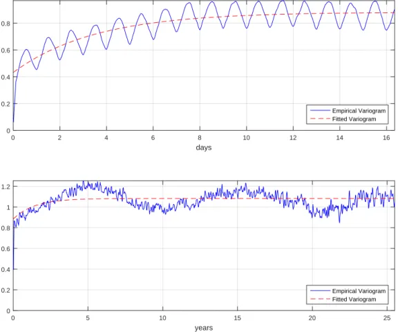
(where Vj(θ) is small). In Figure 1, we present the empirical and the fitted variograms
for the S&P 500, using the discrete model described in Section 2. The dashed line is a fitted exponential obtained by nonlinear weighted least squares regression. It is worth mentioning that, if the variograms in Figure 1 were flat, we would conclude there is no fast and/or slow time scale on the S&P 500 index.
To obtain the sample distribution of the estimated parameters, we bootstrap the pairs of residuals of the non linear regressions solved to obtain the variograms given by Equa-tions (27) and (28). We use the circular block bootstrap of Politis and Romano (1992), with 10,000 bootstrap samples. The block size was chosen according to the procedure de-veloped byPolitis and White(2004). Table1presents the estimated values and standard deviations for the parameters, as well as the 95% bootstrapped confidence interval. The
4
days
0 2 4 6 8 10 12 14 16
0 0.2 0.4 0.6 0.8
Empirical Variogram Fitted Variogram
years
0 5 10 15 20 25
0 0.2 0.4 0.6 0.8 1 1.2
Empirical Variogram Fitted Variogram
Figure 1: The empirical variogram for the S&P 500. The top graph shows the estimate of the variogram model for 5-min log normalized fluctuations after applying a 9 point median filter to compensate for the singular noise log|ǫn|, while the bottom graph shows the empirical variogram
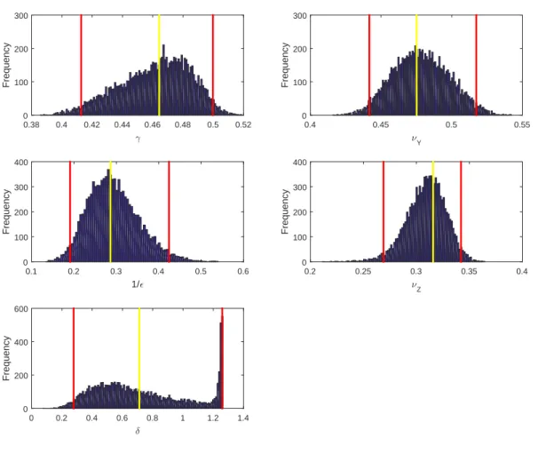
sample distribution of the estimated parameters is shown in Figure 2.
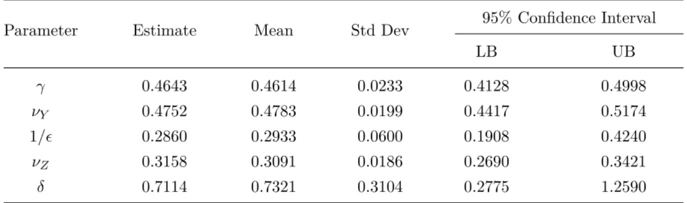
Table 1: Summary statistics of the estimates of the model variogram (36).
Parameter Estimate Mean Std Dev 95% Confidence Interval
LB UB
γ 0.4643 0.4614 0.0233 0.4128 0.4998
νY 0.4752 0.4783 0.0199 0.4417 0.5174
1/ǫ 0.2860 0.2933 0.0600 0.1908 0.4240
νZ 0.3158 0.3091 0.0186 0.2690 0.3421
δ 0.7114 0.7321 0.3104 0.2775 1.2590
Note: This table presents the summary statistics of the estimated parameters of the S&P
500 variogram given by Equation (26). The parameters were estimated using weighted least squares regression. We fit Equation (27) using 5-min data and Equation (28) using 5-day data simultaneously by performing the procedure described in Section2.3. The mean, standard deviation and 95% confidence interval of each parameter were obtained using a circular block boostrap with 10,000 bootstrap samples. LB indicates the lower bound of the confidence interval, while UB indicates the upper bound.
From Table 1, observe that the estimated fast time scale, 1/ǫ, is 0.286, with stan-dard deviation equal to 0.023, meaning an average decoupling time of 3.497 days, with a 95% confidence interval [2.358,5.241]. The estimated slow time scale, δ, is 0.711, which corresponds to a mean-reversion time of 16.868 months, with a confidence in-terval [9.531,43.243]. Notice that these mean-reversion times indicate that the volatility process of the S&P 500 is driven by a fast mean-reverting diffusion and a slowly varying mean-reverting process. The volatility of the invariant distribution of the OU process Y was estimated to be 0.475, while the volatility of the OU processZ was estimated to be 0.316.
Note the oscillatory nature of the variograms in Figure1. This characteristic is related to intra-day variation of volatility, and this was already noticed in Fouque et al. (2000). For a discussion of this cycles from an implicit-volatility viewpoint, see Fouque et al.
(2004).
3.3
Calibration Results
.
0.38 0.4 0.42 0.44 0.46 0.48 0.5 0.52
Frequency
0 100 200 300
8Y
0.4 0.45 0.5 0.55
Frequency
0 100 200 300
1/0
0.1 0.2 0.3 0.4 0.5 0.6
Frequency
0 100 200 300 400
8Z
0.2 0.25 0.3 0.35 0.4
Frequency
0 100 200 300 400
/
0 0.2 0.4 0.6 0.8 1 1.2 1.4
Frequency
0 200 400 600
Figure 2: Bootstrap distributions of the sample parameters obtained by fitting Equations (27) and (28) to two-different datasets. The red line correspond to the estimated parameter, while the red lines correspond to the lower and upper bounds of the 95% bootstrapped confidence interval. In order to obtain the sample distributions, we use the circular block bootstrap of
Politis and Romano (1992) with 10,000 bootstrap samples. The block length was chosen using
implied volatility, given by Equation (32), to market data.
In order to to that, we consider three different models:
• Model 1: in this model, we assume that the volatility is driven by a single mean-reverting OU process, Zt, fluctuating on a slow time scale;
• Model 2: at the opposite extreme, in this model we assume that the volatility process is only driven by a fast mean-reverting OU process, Yt;
• Model 3: in this model, we assume that the volatility is driven by two different factors, one fluctuating on a fast time scale, Yt, and a other fluctuating on a longer
time scale, Zt.
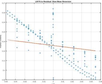
We first look at the performance of Model 1, which considers only a slow volatility factor. In Figure 3a, we show the results of the calibration using only the slow-factor approximation given by Equation (39), which corresponds to assuming ǫ = 0. Corrobo-rating with the findings of Fouque, Papanicolaou, Sircar, and Solna (2011), we observe that Model 1 fails to capture the range of maturities.
In Figure 3b, we look at the performance of Model 2, which uses only the fast-factor approximation given by Equation (38). Again, note that Model 2 fails to capture the range of maturities.
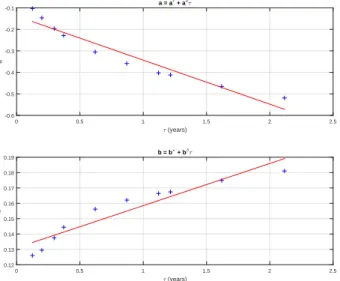
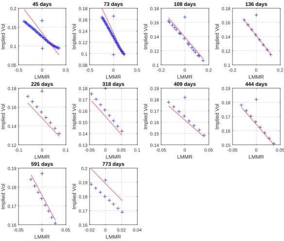
Finally, in fitting the Model 3, which uses the two-factor volatility approximation (32), we follow the two-step procedure ofFouque, Papanicolaou, Sircar, and Solna(2011). First, we fit the skew to obtain ˆai and ˆbi for different maturities τi. In the second stage, these
estimates are then fitted to an affine function ofτ to give estimates ofb∗,bδ,aǫ, andaδ. A
plot of this second term-structure fit on November 03, 2015, is shown in Figure4a along with the calibrated multiscale approximation (32) to all the data on November 03, 2015 in Figure4b.
From Figure4b, note that the ability of Model 3 to capture the range of maturities is much improved when compared to Models 1 and 2. Thus, the two-scale volatility model with its additional parameters performs better than either of the one-scale models.
Table 2reports the estimated parameters of the correction to the Black-Scholes price for each one of the three models presented in this section. Observe that in the regime where our approximation is valid, the parameters aǫ,aδ, andbδ are expected to be small,
LM
-0.05 -0.04 -0.03 -0.02 -0.01 0 0.01 0.02 0.03 0.04 0.05
Implied Volatility
0.09 0.1 0.11 0.12 0.13 0.14 0.15 0.16
0.17 LM Fit to Residual: Slow Mean Reversion
(a) τ-adjusted implied volatility I−bδτ.
LMMR
-0.4 -0.3 -0.2 -0.1 0 0.1 0.2 0.3 0.4
Implied Volatility
0.08 0.1 0.12 0.14 0.16 0.18
0.2 Pure LMMR Fit: Fast Mean Reversion
(b) S&P 500 implied volatilities.
Figure 3: Data and calibrated fit on November 03, 2015. In Figure (a), we plot the maturity adjusted implied volatility as a function of the log-moneyness, LM. The plus signs are from S&P 500 data and the lineσ∗+aδ(LM) shows the fit using the estimated parameters from only a slow
factor fit using ordinary least squares regression. In figure (b), we present the S&P 500 implied volatilities as a function of the LMMR. The plus signs are from S&P 500 data, and the line b∗+aǫ(LMMR) shows the result using the estimated parameters from only a fast factor fit using
= (years)
0 0.5 1 1.5 2 2.5
a
-0.6 -0.5 -0.4 -0.3 -0.2
-0.1 a = a
0
+ a/ =
= (years)
0 0.5 1 1.5 2 2.5
b
0.12 0.13 0.14 0.15 0.16 0.17 0.18
0.19 b = b
$ + b/=
(a) Term-structure fits.
LMMR
-0.4 -0.3 -0.2 -0.1 0 0.1 0.2 0.3 0.4
Implied Vol
0.06 0.08 0.1 0.12 0.14 0.16 0.18
0.2 Fitted Surface and Data
(b) Data and calibrated fit.
Figure 4: Data and calibrated fit on November 03, 2015. In Figure (a), the plus signs in the top plot are the slope coefficientsai of LMMR fitted in the first step of the regression. The solid
line is the straight line (aǫ+aδτ) fitted in the second step of the regression. The bottom plot shows the corresponding picture for the skew interceptsbi fitted to the straight lineb∗+bδτ. In
LMMR
-0.5 0 0.5
Implied Vol
0.05 0.1 0.15
0.2 45 days
LMMR
-0.5 0 0.5
Implied Vol 0.08 0.1 0.12 0.14 0.16
0.18 73 days
LMMR
-0.2 0 0.2
Implied Vol
0.1 0.12 0.14 0.16
0.18 108 days
LMMR
-0.2 0 0.2
Implied Vol
0.1 0.12 0.14 0.16
0.18 136 days
LMMR
-0.1 0 0.1
Implied Vol
0.12 0.14 0.16
0.18 226 days
LMMR
-0.05 0 0.05 0.1
Implied Vol 0.13 0.14 0.15 0.16 0.17
0.18 318 days
LMMR
-0.05 0 0.05
Implied Vol 0.14 0.15 0.16 0.17 0.18
0.19 409 days
LMMR
-0.05 0 0.05
Implied Vol
0.15 0.16 0.17 0.18
0.19 444 days
LMMR
-0.05 0 0.05
Implied Vol
0.16 0.17 0.18
0.19 591 days
LMMR
-0.02 0 0.02 0.04
Implied Vol
0.16 0.17 0.18 0.19
0.2 773 days
on November 03, 2015.
Table 2: Estimated values of the group market parameters
σ∗ aǫ aδ b∗ bδ Vδ
0 V1δ V3ǫ
Model 1 0.1257 -0.1223 0.0308 0.0313 -0.0019
Model 2 0.1434 -0.1192 0.1426 -0.0004
Model 3 0.1318 -0.1383 -0.2049 0.1311 0.0274 0.0285 -0.0035 -0.0003
Note: In this table, we report the estimated parameters from the fit of implied volatilities
to log-moneyness to maturity ratio for every model on November 03, 2015. For Models 1 and 2, we fit Equations (38) and (39) to data using ordinary least squares regression. The estimated parameters for Model 3 result from the fit of Equation (32) to data following the 2-step procedure suggested by Fouque, Papanicolaou, Sircar, and Solna (2011). The last three columns were obtained through the inversion of Equations (34) to (37).
In Table3, we compare the adjustment of the three models presented in this section to the market prices using the absolute percentage error|Pobserved−Pmodel|/Pobserved, where Pmodel is the price given by the model and Pobserved is the observed market price of the option. Since the volatility used to obtain the Black-Scholes prices differs in every model, we are not able to compare them unless we use the same volatility in the Black-Scholes formula across all the models.
In order to compare the corrected prices for all the three models, we calculate the historical volatility of the returns of the S&P 500. First, we obtain a time-series of historical volatilities on this index by using a rolling-window of 63 days (three-months) during one year. Then, we use the average of this time-series as our estimator of the historical volatility, ¯σ. For the time period from October 23, 2014, to October 23, 2015, the estimated historical volatility in the S&P 500 was 14%. In Panel A, we report the percentage of times in which the model in question presented the best adjustment when compared to the observed market prices. Since our model provides only corrected call prices, we use the put-call parity in order to obtain the put prices with the same strike and time to maturity. Note that, for call prices, Model 1 presents the best adjustment to data, while for put prices, Model 3 provides the best fit, followed by the Black-Scholes model.
we compare the adjustment of Model 3 to data, although the magnitudes are different. Finally, in Panel C we compare the adjustment of Model 2 to data. In this case, the Black-Scholes model performs better when we look at put prices. For call prices, Model 2 presents the best adjustment.
Notice that, when we compare the prices given by every model to the Black-Scholes prices, we find opposite results for call and put prices. This may be an evidence that the put-call parity does not hold, even in perfectly liquid markets as the American market.
Table 3: Comparison of prices generated by the models and observed market prices
Model Call Prices Put Prices
Panel A: Model Comparison using Historical Volatility
Model 1 36.3636 13.5802
Model 2 16.2338 17.9012
Model 3 29.8701 37.6543
Black-Scholes 17.5325 30.8642
Panel B: Model 1 versus Black-Scholes
Model 1 4.5455 96.2963
Black-Scholes 95.4545 3.7037
Panel C: Model 2 versus Black-Scholes
Model 2 56.4935 47.5309
Black-Scholes 43.5065 52.4691
Panel D: Model 3 versus Black-Scholes
Model 3 31.1688 71.6049
Black-Scholes 68.8312 28.3951
Note: In this table, we compare the adjustment of each model to the observed market prices
of the options. In Panel A, we compute the Black-Scholes prices using the historical volatility ¯
σ = 0.14. From Panel B to Panel D, we compute the Black-Scholes prices using the effective volatilityσ∗ estimated from every model. All the values are expressed in percentage terms.
3.4
Simulating Derivative Prices
data and also when we try to estimate using the wrong model (wrong number of scales, for example). We will also test the performance of the algorithm under different sample sizes and parameter settings.
We will denote asN∗ the true number of volatility scales that generate the data, while N will be the value with which we do the estimation. We will generate synthetic data under four possible parameter settings:
• Setting A: The first data set will be obtained by generating the option prices with the Black–Scholes formula (29), assuming a constant volatility.
• Setting B: The second data set will be obtained by generating the option prices assuming that Model 1 is the Data Generating Process (DGP) and N∗ = 1.
• Setting C: The third data set will be obtained by generating the option prices using Model 2 as the GDP, which assumes that N∗ = 1.
• Setting D: Finally, the fourth data set will be obtained by generating the options prices with Model 3 as the DGP and N∗ = 2.
In the estimation, we will useN = 1 orN = 2, with two different sample sizes: T = 500 orT = 1000. Note that any combination of the above forms an experiment.
4
Application: Pricing an Exotic Derivative
In this section, we present an application of the model for pricing a binary or digital option with no exercise option, using the calibration obtained in Section 3.3 for options in and close to the money.
Consider a cash-or-nothing call that pays a fixed amount Q on the dateT if XT > K,
and zero otherwise. Its payoff function is
h(x) = Q1{x>K}, (42)
where1A is the indicator function of a set A.
According to the perturbation theory developed in Fouque, Papanicolaou, Sircar, and Solna(2011), the stochastic volatility-corrected price is given by
˜
where
P1(t, x, z) = (T −t) V0δ ∂ ∂σ +V
δ
1D1 ∂ ∂σ
! +Vǫ
3D1D2 !
P∗
BS, (44)
and P∗
BS =Qe−r(T−t)N(d2).
Using the simulated prices from Section 3.4, the goal of this section is to obtain the prices of this exotic derivative under the four different settings considered in the last section, and then compare the models across different scenarios.
5
Concluding Remarks
The main idea of the asymptotic models of Fouque, Papanicolaou, Sircar, and Solna
(2011) is to use perturbation techniques to correct constant volatility models in order to capture the effects of stochastic volatility. In this paper, we compare the performance of three different specifications of the Fouque, Papanicolaou, and Sircar (2000) stochastic volatility model for pricing European call options with the Black-Scholes model. So far, we have found no evidence that these asymptotic models perform better than the Black-Scholes model. Moreover, we find opposite results when we apply this theory to pricing call and put options, what may indicate that the put-call parity does not hold.
FollowingFouque, Papanicolaou, and Sircar (2000), we derive a first-order asymptotic approximation for European options under multiscale stochastic volatility models with fast and slow factors. The price approximation was translated to an implied volatility surface approximation which is linear in log-moneyness. We show that the extracted pa-rameters (group market papa-rameters) are small, in accordance with the asymptotic analysis developed by these authors.
We use S&P 500 data to demonstrate that the volatility of this index is driven by two diffusions: one fast mean-reverting and one slow-varying. We find a fast time scale of 3.5 days, and a slow time scale of 16.9 months. These time-scales are statistically significant, and therefore cannot be ignored in option pricing and hedging.
References
Alizadeh, S., M. W. Brandt, and F. X. Diebold. 2002. Range-based estimation of stochas-tic volatility models. Journal of Finance 06:1047–1092.
Andersen, T. G., and T. Bollerslev. 1997. Intraday Periodicity and Volatility Persistence in Financial Markets. Journal of Empirical Finance 4:115–158.
Black, F., and M. Scholes. 1973. The Pricing of Options and Corporate Liabilities.Journal of Political Economy 81:7637–659.
Chernov, M., R. Gallant, E. Ghysels, and G. Tauchen. 2003. Alternative models for stock price dynamics. Journal of Econometrics 116:225–257.
Chronopoulou, A., and F. G. Viens. 2012. Estimation and pricing under long-memory stochastic volatility. Annals of Finance 8:379–403.
Cressie, N. 1985. Fitting variogram models by weighted least squares. J. Int. Ass. Math. Geol. 17:563–586.
Engle, R. F. 1982. Autoregressive conditional heteroskedasticity with estimates of the variance of U.K. inflation. Econometrica 50:987–1008.
Engle, R. F., and A. Patton. 2001. What good is a volatility model? Quantitative Finance
1:237–245.
Figlewski, S. 2009. Estimating the Implied Risk Neutral Density for the U.S. Market Portfolio. In Volatility and Time Series Econometrics: Essays in Honor of Robert F. Engle. Oxford University Press.
Fouque, J. P., G. Papanicolaou, and K. R. Sircar. 2000. Derivatives in Financial Markets with Stochastic Volatility. NY: Cambridge University Press.
Fouque, J. P., G. Papanicolaou, K. R. Sircar, and K. Solna. 2003a. Short time-scale in S&P 500 volatility. Journal of Computational Finance 6:1–23.
Fouque, J. P., G. Papanicolaou, K. R. Sircar, and K. Solna. 2003b. Singular Perturbations in Option Pricing. SIAM Journal on Applied Mathematics 63:1648–1681.
Fouque, J. P., G. Papanicolaou, K. R. Sircar, and K. Solna. 2004. Maturity cycles in implied volatility. Finance and Stochastics 8:451–477.
Fouque, J. P., G. Papanicolaou, R. Sircar, and K. Solna. 2011. Multiscale Stochastic Volatility for Equity, Interest-Rate and Credit Derivatives. USA: Cambridge University Press.
Gatheral, J. 2006. The Volatility Surface: a Practitioner’s Guide. Inc: John Wiley and Sons.
Heston, S. L. 1993. A Closed-Form Solution for Options with Stochastic Volatility with Applications to Bond and Currency Options. The Review of Financial Studies 6:327– 343.
Hillebrand, E. 2005. Neglecting parameter changes in GARCH models.Journal of Econo-metrics 1-2:121–138.
LeBaron, B. 2001. Stochastic volatility as a simple generator of apparent financial power laws and long memory. Quantitative Finance 1:621–631.
Machuca, G. E. G. 2010. Volatilidade Estocástica Multiescala: Modelagem, Estimação e Aplicação com Preços da Petrobras. Master Thesis, IMPA.
Merton, R. C. 1969. Lifetime portfolio selection under uncertainty: The continuous-time case. Review of Economics and Statistics 51:247–257.
Politis, D. N., and J. P. Romano. 1992. A circular block-resampling procedure for sta-tionary data. In R. LePage and L. Billard (eds.), Exploring the Limits of Bootstrap, pp. 263–270. New York: John Wiley.
Appendix
A
Properties of the Variogram Estimator
In this section, we will study some properties of the variogram estimator given by Equation (26). In order to do that, consider the following lemmas:
Lemma 1. Let s < t, then
Eh(Yt−E[Yt]) (Ys−E[Ys])
i
=νY2e−α(t−s)1−e−2αs, (A.1)
Eh(Zt−E[Zt]) (Zs−E[Zs])
i
=νZ2e−δ(t−s)1−e−2δs. (A.2)
Proof.
Eh(Zt−E[Zt]) (Zs−E[Zs])
i
=E νY √
2α Z t
0 e
−α(t−u)dW(1)
u νZ
√
2α Z s
0 e
−α(s−u)dW(1)
u
= 2ανY2e−α(t+s)E Z t
0 e
αudW(1)
u
Z s
0 e
αu)dW(1)
u
= 2ανY2e−α(t+s)E Z s
0 e
αudW(1)
u
Z s
0 e
αudW(1)
u +
+ 2ανY2e−α(t+s)E Z t
s e
αudW(1)
u
Z s
0 e
αudW(1)
u
= 2ανY2e−α(t+s)E Z t
0 e
αudW(1)
u
Z s
0 e
αudW(1)
u
= 2ανY2e−α(t+s)E Z t
0 e
αudW(1)
u
2
= 2ανY2e−α(t+s)E Z t
0 e
2αudt2
=νY2e−α(t+s)(e2αs−1) =νZ2e−δ(t−s)1−e−2δs.
Similarly, we can get (A.1).
By using the previous Lemma, we can conclude that
Ehlogf1( ¯Yj) logf1( ¯Y0) i
≈ν2
Ye−αj∆t,
Similarly, we have
Ehlogf1( ¯Zj) logf1( ¯Z0)
i
≈νZ2e−αj∆t,
Ehlogf1( ¯Z)2i≈νZ2, (A.4)
where ¯Y and ¯Z denote the asymptotic distributions of the OU processes given by (1).
Lemma 2. For the model presented in this paper, if s < t, then
Eh(Yt−E[Yt]) (Zs−E[Zs])
i = 2
√α√δ
α+δ ρ1˜,2νYνZ
e−α(t−s)−e−αte−δs. (A.5)
Otherwise, if s > t,
Eh(Yt−E[Yt]) (Zs−E[Zs])
i = 2
√
α√δ
α+δ ρ1˜,2νYνZ
e−δ(s−t)−e−αse−δt. (A.6)
Proof. Suppose thats < t, then
Eh(Yt−E[Yt]) (Zs−E[Zs])
i
=E νY √
2α Z t
0 e
−α(t−u)dW˜(1)
u νZ
√
2δρ1˜,2 Z s
0 e
−δ(s−u)dW˜(1)
u
+E νY √
2α Z t
0 e
−α(t−u)dW˜(1)
u νZ
√
2δq1−ρ1˜,2 Z s
0 e
−δ(s−u)dW˜(2)
u
=E νY √
2α Z s
0 e
−α(t−u)dW˜(1)
u νZ
√
2δρ1˜,2 Z s
0 e
−δ(s−u)dW˜(1)
u
+E νY √
2α Z s
0 e
−α(t−u)dW˜(1)
u νZ
√
2δq1−ρ1˜,2 Z s
0 e
−δ(s−u)dW˜(2)
u
=√2ανY √
2δνZρ1˜,2e−αte−δs
Z s
0 e
(α+δ)udu
= 2
√
α√δ
α+δ νYνZρ1˜,2e
−αte−δs
e(α+δ)s−1
= 2
√α√δ
α+δ ρ1˜,2νYνZ
e−δ(s−t)−e−αse−δt.
By following Fouque, Papanicolaou, Sircar, and Solna (2011) and using the previous Lemma, we get
Ehlogf1( ¯Y) logf2( ¯Z)i≈ 2
√
α√δ
α+δ ρ1˜,2νYνZ, (A.7)
Ehlogf1( ¯Yj) logf2( ¯Z0)
i
≈ 2 √
α√δ
α+δ ρ1˜,2νYνZe
−αj∆t, (A.8)
Ehlogf1( ¯Y0) logf2( ¯Zj)
i
≈ 2 √
α√δ
α+δ ρ1˜,2νYνZe
Proposition 1.
En(Fn+j −Fn)2
o
≈2c2Y + 2νY2(1−e−αj∆t) + 2νZ2(1−e−δj∆t)+
+ 4
√
α√δ
α+δ ρ1˜,2νYνZ
2−e−αj∆t−e−δj∆t.
(A.10)
Proof.
En(Fn+j −Fn)2
o
=En(Fj −F0)2
o
=Enh logf1( ¯Yj)−logf1( ¯Y0)
+logf2( ¯Zj)−logf2( ¯Z0)
io + +Enh(log|ǫj | −log|ǫ0 |)
io
=En logf1( ¯Yj)−logf1( ¯Y0)
o
+En logf2( ¯Zj)−logf2( ¯Z0)
o + +En(log|ǫj | −log|ǫ0 |)
o +
+ 2En logf1( ¯Yj)−logf1( ¯Y0) logf2( ¯Zj)−logf2( ¯Z0)
o
= 2Enlogf1( ¯Y)2 o
−2Enlogf1( ¯Yj) logf1( ¯Y0) o
+ 2Enlogf2( ¯Z)2 o
−2Enlogf2( ¯Zj) logf2( ¯Z0)
o
+ 2Var (log (¯ǫ)) + 4Enlogf1( ¯Y0) logf2( ¯Z)o
−2Enlogf1( ¯Yj) logf2( ¯Z0)
o
−2Enlogf1( ¯Y0) logf2( ¯Z)o
≈2c2Y + 2νY2 1−e−αj∆t+ 2νZ2 1−e−δj∆t+8
√
α√δ
α+δ ρ1˜,2νYνZ
− 4 √
α√δ
α+δ ρ1˜,2νYνZe −αj∆t
−4 √
α√δ
α+δ ρ1˜,2νYνZe −δj∆t
≈2c2Y + 2νY2 1−e−αj∆t+ 2νZ2 1−e−δj∆t+
+ 4
√
α√δ
α+δ ρ1˜,2νYνZ
2−e−αj∆t−e−δj∆t
In the previous proof, we used Equations (A.3), (A.4), and Equations (A.7) to (A.9). Since we assume thatδ≪1/ǫ, by Equation (A.10) we have that
√
α√δ α+δ ≈
√
α√δ
α ≈
√
δ
√
α ≈0. (A.11)
B
First-Order Perturbation Theory
In this section, we derive the asymptotic approximation for options prices of Fouque, Papanicolaou, and Sircar (2000). In order to derive the corrected prices, as the terms associated withδ are small when δ →0 and give rise to a regular perturbation problem, we first expand Pǫ,δ in powers of√δ:
Pǫ,δ =P0ǫ+√δP1ǫ+δP2ǫ+. . . . (B.1)
We insert the above expansion in equation (9) (both the PDE and the terminal condi-tion), grouping generators in term of powers ofδ in the form
1 ǫL0+
1
√ǫL1+L2 !
P0ǫ+√δ
1 ǫL0+
1
√ǫL1+L2 !
P1ǫ+ M1+ 1
√ǫM3 !
P0ǫ
+. . .= 0.
(B.2)
Write Lǫ,δ and Pǫ,δ as
Lǫ,δ =Lǫ+√δMǫ+δM2, (B.3)
Pǫ,δ =X
j≥0
(√δ)jPjǫ, (B.4)
where
Lǫ = 1 ǫL0+
1
√
ǫL1 +L2, (B.5)
Mǫ = √1
ǫM3+M1, (B.6)
Pjǫ =X
i≥0
(√ǫ)iPi,j. (B.7)
Inserting (B.1) in (9) and collecting term of like-powers of√δ, we find that the lowest order equations of the regular perturbation expansion are
O(1) : 0 =LǫP0ǫ, (B.8)
O(√δ) : 0 =LǫP1ǫ+MǫP0ǫ, (B.9)
O(δ) : 0 =LǫP2ǫ+MǫP1ǫ+M2P0ǫ. (B.10)
con-ditions 1
ǫL0+
1 √
ǫL1+L2
Pǫ
0 = 0, Pǫ
0(T, x, y, z) = h(x).
(B.11) 1
ǫL0+
1 √
ǫL1+L2
Pǫ
1 =−
M1+√1ǫM3
Pǫ
0, Pǫ
1(T, x, y, z) = 0,
(B.12)
where the terminal payoff is assigned to the independent term Pǫ
0. Next, we expand P0ǫ and Pǫ
1 in powers of
√
ǫ.
B.0.1 Zeroth-Order Approximation P0
From a fast factor expansion of equation (9), we will find the zeroth order term P0,0, in our approximation (18).
Consider the expansion of Pǫ
0 in powers of√ǫ:
Pǫ
0 =P0+√ǫP1,0 +ǫP2,0+ǫ3/2P3,0+. . . . (B.13)
By inserting (B.13) in (9) and rearranging terms, we get
1
ǫL0P0 + 1
√
ǫ(L0P1,0+L1P0) + (L0P2,0+L1P1,0+L2P0) + +√ǫ(L0P3,0+L1P2,0+L2P1,0) +. . .= 0.
(B.14)
By collecting term of like-powers of √ǫ, we get
O
1 ǫ
: L0P0 = 0, (B.15)
O √1
ǫ !
: L0P1,0+L1P0 = 0, (B.16)
O(1) : L0P2,0+L1P1,0+L2P0 = 0, (B.17)
O√ǫ: L0P3,0+L1P2,0+L2P1,0 = 0. (B.18)
automatically be satisfied. Hence, we seek solutions of the form:
P0,0 =P0,0(t, x, z), (B.19) P1,0 =P1,0(t, x, z). (B.20)
Note that Equation (B.17) is a Poisson equation for P2,0 with respect to y. For there be a solution,L2P0 must satisfy the solvability condition:5
hL2P0i= ∂P0 ∂t +
1 2σ¯
2x2∂2P0
∂x2 +r x ∂P0
∂x −P0 !
= 0, (B.21)
which is the Black-Scholes pricing operatorL(¯σ(z)) with effective averaged volatility ¯σ(z):
¯
σ(z) =hf2(·, z)i=Z f2(y, z)Φ(dy), (B.22)
where the level z of the slow factor appears as a parameter. Therefore, the leading-order termP0(t, x, z) =PBS(t, x; ¯σ(z)) is the Black-Scholes price at volatility ¯σ(z), which
satisfies the following PDE and terminal condition:
LBS(¯σ(z))PBS = 0,
PBS(T, x; ¯σ(z)) = h(x).
(B.23)
B.0.2 Fast Time Scale Correction Pǫ
1,0
The order √ǫ in (B.18) give the following Poisson equation for P3,0:
L0P3,0+L1P2,0+L2P1,0 = 0. (B.24)
The solvability condition for this equation is given by
hL2P1,0+L1P2,0i= 0. (B.25)
5
Note that Equations (B.17) and (B.18) are Poisson equations of the form 0 =L0+χ,
By the Fredholm alternative, the equation above, which is a linear ODE iny, admits a solutionP in
L2
(Φ) only if the following solvability, or centering, condition holds:
hχi ≡
Z
χ(y)Φ(dy) = 0,
LetDk be defined as
Dk=xk
∂k
∂xk, (B.26)
then, introducing a solutionφ(y, z) to the Poisson equation L0φ= f2− hf2i, we deduce the following expression forP2,0:
P2,0(t, x, y, z) =− 1
2φ(y, z)D2P0,0(t, x, y, z) +c(t, x, z), (B.27)
up to an additive functionc(t, x, z) which does not depend ony. Then, by using Equations (11) and (12) and the fact that P1,0 does not depend on y, we find that P1ǫ satisfied the following PDE:
LBS(¯σ(z))P1ǫ =AǫPBS;
Pǫ
1(T, x;z) = 0;
(B.28)
where thez-dependent operatorAǫ =√ǫhL
1L−01(L2− hL2i)i. Using Equation (B.17), we can rewriteAǫ as
Aǫ=−V3ǫ(z)D1D2−V2ǫ(z)D2, (B.29)
where the two group parametersVǫ
2(z) and V3ǫ(z) are given by
V2ǫ(z) =−ρ1
√
ǫ
2 hβf(·, z) ∂φ
∂y(·, z)i, (B.30)
V3ǫ(z) =−
√ǫ
2 hβΛ1(·, z) ∂φ
∂y(·, z)i. (B.31)
With the previous notation, we have
LBS(¯σ(z)) =
∂ ∂t+
1 2σ¯(z)
2D2+r(D1
− ·). (B.32)
Therefore, the first-order fast scale correction termP1,0(t, x, z) is given in terms ofPBS
by
P1ǫ,0(t, x, z) = −(T −t)AǫPBS(t, x; ¯σ(z)). (B.33)
B.0.3 Slow Time Scale Correction Pδ
0,1