S&P 500 OPTIONS
Pedro Santa-Clara and Shu Yan*
Abstract—We use a novel pricing model to imply time series of diffusive volatility and jump intensity from S&P 500 index options. These two measures capture the ex ante risk assessed by investors. Using a simple general equilibrium model, we translate the implied measures of ex ante risk into an ex ante risk premium. The average premium that compensates the investor for the ex ante risks is 70% higher than the premium for realized volatility. The equity premium implied from option prices is shown to significantly predict subsequent stock market returns.
I. Introduction
T
HIS paper uses option prices to estimate the risk of the stock market as it is perceived ex ante by investors. We consider two types of risk in stock prices: diffusion risk and jump risk.1As Merton (1980) argued, diffusion risk can be accurately measured from the quadratic variation of the realized price process. In contrast, since even high-probability jumps may fail to materialize in sample, the ex ante jump risk perceived by investors may be quite different from the ex post realized variation in prices. Therefore, studying measures of realized volatility and realized jumps from the time series of stock prices will give us a limited picture of the risks investors fear. Fortunately, since options are priced on the basis of ex ante risks, they give us a privileged view of the risks perceived by investors. Using option data solves the “peso problem” in measuring jump risk from realized stock returns.In our model, both the volatility of the diffusion shocks and the intensity of the jumps vary over time following separate stochastic processes.2Our model is quadratic in the state variables. This allows the covariance structure of the shocks to the state variables to be unrestricted, which proves
to be important in the empirical analysis. We are still able to solve for the European option prices in a manner similar to the affine case of Duffie, Pan, and Singleton (2000). In the empirical application, the model is shown to produce pric-ing errors of the order of magnitude of the bid-ask spread in option prices.
When we calibrate the model to S&P 500 index option prices from the beginning of 1996 to the end of 2002, we obtain time series of the implied diffusive volatility and jump intensity. We find that the innovations to the two risk processes are not very correlated with each other, although both are negatively correlated with stock returns. The two components of risk vary substantially over time and show a high degree of persistence. The diffusive volatility process varies between close to 0 and 36% per year, which is in line with the level of ex post risk measured from the time series of stock returns. The jump intensity process shows even wider variation. Sometimes the probability of a jump is 0, while at other times it is more than 99%.3We estimate that the expected jump size is⫺9.8%. Interestingly, we do not observe any such large jumps in the time series of the S&P 500 index in our sample, not even around the times when the implied jump intensity is very high. These were there-fore cases in which the jumps that were feared did not materialize. However, the perceived risks are still likely to have affected the expected return in the stock market at those times.
To investigate the impact of ex ante risk on expected returns, we solve for the stock market risk premium in a simple economy with a representative investor with power utility for final wealth. We find that the equilibrium risk premium is a function of both the stochastic volatility and the jump intensity. Given the implied stochastic volatility and jump intensity processes, together with the estimated coefficient of risk aversion for the representative investor, we estimate the time series of the ex ante equity premium. This is the expected excess return demanded by the investor to hold the entire wealth in the stock market when facing the diffusion and jump risks implicit in option prices. We decompose the ex ante equity premium into compensation for diffusive risk and compensation for jump risk. We find the ex ante equity premium to be quite variable over time. In our sample, the equity premium demanded by the repre-sentative investor varies from as low as 0.3% and as high as 54.9% per year! The compensation for jump risk is on
Received for publication January 19, 2007. Revision accepted for publication July 29, 2008.
* Santa Clara: Universidade Nova de Lisboa and NBER; Yan: Univer-sity of South Carolina.
We thank Julio Rotemberg (the editor), two anonymous referees, Ravi Bansal, David Bates, Michael Brandt, Michael Brennan, Joa˜o Cocco, Marcelo Fernandes, Mikhail Chernov, Christopher Jones, Jun Liu, Francis Longstaff, Jun Pan, Alessio Saretto, and Bill Schwert for helpful com-ments. We also thank seminar participants at Instituto de Empresa (Ma-drid), Universidade Nova de Lisboa, University of Arizona, University of South Carolina, University of Vienna, the Fifteenth FEA Conference at USC, the NBER Spring 2008 Asset Pricing Meeting, the 2008 Luso-Brazilian Finance Meeting, and the University of Amsterdam Fourth Annual Empirical Asset Pricing Retreat. An appendix with derivations of some expressions in the paper and some additional results is available online at http://www.mitpressjournals.org/doi/suppl/10.1162/rest.2010. 11549.
1There is ample empirical evidence for this kind of specification. See,
for example, Jorion (1988), Bakshi, Cao, and Chen (1997), and Bates (2000).
2In contrast, other jump-diffusion models impose a constant jump
intensity (Merton, 1976; Bates, 1996) or make it a deterministic function of the diffusive volatility (Bates, 2000; Duffie, Pan, & Singleton, 2000; Pan, 2002). The empirical analysis shows that the jump intensity varies a lot and that although it is related to the diffusive volatility, it has its own source of shocks.
3We calculate this probability as 1⫺e⫺, whereis the instantaneous jump intensity. This calculation assumes that the jump intensity remains constant for an entire year. Since the process we estimate for the jump intensity is strongly mean reverting, this figure overstates the probability of a jump during the year.
The Review of Economics and Statistics,May 2010, 92(2): 435–451
average more than half of the total premium. Moreover, in times of crisis, the jump risk commands a premium of 45.4% per year and can be close to 100% of the total premium.4
The ex ante premium evaluated at the average levels of diffusive volatility and jump intensity implied from the options in our sample is 11.8%. In contrast, the same investor would require a premium of only 6.8% as compen-sation for the realized volatility (i.e., the sample standard deviation of returns) during the same sample period. There-fore, the required compensation for the ex ante risks is more than 70% higher than the compensation for the realized risks! This finding supports the peso explanation of the equity premium puzzle proposed by Rietz (1988), Brown, Goetzmann, and Ross (1995), and Barro (2006).
According to this explanation, there is a risk of a sub-stantial crash in the stock market that has not materialized in the sample but justifies a larger risk premium than what has traditionally been thought reasonable along the lines of Mehra and Prescott (1985).
To show that the equity premium implied from the op-tions market is indeed related to stock prices, we run predictive regressions of stock returns on the lagged implied equity premium. We find that the regression coefficient is significant for different predictability horizons. For
one-month returns, the R2 is 4.1%, and it becomes 6.6% for
three-month returns. The regression coefficient is close to 1 for the three-month horizon as expected for an unbiased forecast. Finally, we examine the relation between the option implied equity premium and three variables related to financial crises: the T-bill rate, the spread of bank com-mercial paper over T-bills, and the spread of high-yield bonds over Treasuries. Intuitively, the jump risk we uncover in options should be related to large-scale financial crises in which the Fed lowers interest rates, interbank loans dry up and become more expensive, and corporations are more likely to default. We find significant relations between these
variables and the implied equity premium, with an R2 as
high as 13.9% for the high-yield spread.
The paper closest to ours is Pan (2002).5She estimates a jump-diffusion model from both the time series of the S&P 500 index and its options from 1989 to 1996. She uses the pricing model proposed by Bates (2000) which has a square root process for the diffusive variance and jump intensity proportional to the diffusive variance. The jump risk pre-mium is specified to be linear in the variance. Pan finds a significant jump premium of roughly 3.5%, which is of the same order of magnitude of the volatility risk premium of
5.5%. The main difference between our paper and hers is that in Pan’s framework, it is hard to disentangle the diffusion and jump risks and risk premia since they are all driven by a single state variable, the diffusive volatility.
Finally, a word of caution. Our analysis relies on option prices, and, of course, options may be systematically mis-priced. That would bias our ex ante risk measures. Coval and Shumway (2001) and Driessen and Maenhout (2003) report empirical evidence that some option strategies have unusually high Sharpe ratios, which may indicate mispric-ing. Santa-Clara and Saretto (2004) show that transaction costs and margin requirements impose substantial limits to arbitrage in option markets, which may allow mispricings to persist.
The paper proceeds as follows. In section II, we present the dynamics of the stock market index under the objective and the risk-adjusted probability measures, and we derive an option pricing formula. In section III, we discuss the data and the econometric approach. The model estimates and its performance in pricing the options in the sample are cov-ered in section IV. Section V contains the main results of the paper, the analysis of the risks implied from option prices and what they imply for the equity premium. Section VI concludes.
II. The Model
In this section we introduce a new model of the dynamics of the stock market return that displays stochastic diffusive volatility and jumps with stochastic intensity. We derive the equilibrium stock market risk premium in a simple economy with a representative investor with CRRA utility. This risk premium compensates the investor for both volatility and jump risks. We also obtain the risk-adjusted dynamics of the stock, volatility, and jump intensity processes and use them to price European options.
A. Stock Market Dynamics
We model the dynamics of the stock market index with two sources of risk: diffusive risk, captured by a Brownian motion, and jump risk, modeled as a Poisson process. The diffusive volatility and the intensity of the jump arrivals are stochastic and interdependent. We parameterize the pro-cesses as:
dS⫽共r⫹⫺Q兲Sdt⫹YSdWS⫹QSdN (1)
dY⫽共Y⫹YY兲dt⫹YdWY (2)
dZ⫽共Z⫹ZZ兲dt⫹ZdWZ (3)
ln (1⫹Q)⬃ᏺ
冉
ln共1⫹Q兲⫺1 2Q2, Q
2
冊
(4)Prob共dN⫽1兲⫽dt, where⫽Z2 (5)
4This variation in the equity premium is extreme and may be due to
overfitting a particular equilibrium model. It also assumes that option prices reflect accurately investors’ expectations. These potential limita-tions are further discussed in section VB.
5Other related work includes Ait-Sahalia, Wang, and Yared (2001),
⌺⫽
冉
1 SY SZ
SY 1 YZ
SZ YZ 1
冊
. (6)
WS, WY, and WZ are Brownian motions with constant
correlation matrix⌺, andNis a Poisson process with arrival intensity.Qis the percentage jump size and is assumed to follow a displaced log-normal distribution independently over time. This guarantees that the jump size cannot be less than⫺1 and therefore that the stock price remains positive
at all times. We assume that N and Q are independent of
each other and that Q is independent of the Brownian
motions. The instantaneous variance of the stock return is
V⫽Y2.ris the risk-free interest rate, assumed constant for convenience. We also assume that the stock pays no divi-dends, although it would be trivial to accommodate them by adding a term in the drift of the stock price. is the risk premium on the stock, which we show below to be a function ofY andZ. Finally, the termQadjusts the drift for the average jump size.
In our model, the stock price, the stochastic volatility, and the jump intensity follow a joint quadratic jump-diffusion
process where the stochastic processes ofV and are the
squares of linear (gaussian) processes ofY andZ, respec-tively.6 Applying Ito’s lemma, we can write the processes followed byVand:
dV⫽共Y 2
⫹2YY⫹2YY2兲dt⫹2YYdWY (7)
d⫽共Z2
⫹2ZZ⫹2ZZ2兲dt⫹2ZZdWZ. (8)
The drift and diffusion terms in equations (7) and (8) depend on the signs of the gaussian state variablesYandZ.
Note that the instantaneous correlation betweendSanddV
is constant,SY, while the instantaneous correlation between
dSanddY is sgn (Y)SYwhere sgnis the sign function, since公V ⫽ sgn (Y)Y and公 ⫽sgn (Z)Z.7
Without the jump component, our model collapses to a stochastic volatility model similar to that of Stein and Stein (1991).8It can easily be seen that the model does not belong to the affine family of Duffie et al. (2000), in that the drifts
and the covariance terms in V and are not linear in the
state variables. For instance, the covariance betweendVand
d isYYZYZ.
Our model belongs to the family of linear-quadratic jump-diffusion models. It is the first model in which the jump intensity follows explicitly its own stochastic pro-cess. In contrast, existing jump diffusion models either assume that the jump intensity is constant or make it a deterministic function of other state variables such as sto-chastic volatility.9 For instance, Pan (2002) assumes that is a linear function ofV. It is of course an empirical issue whether the jump intensity is completely driven by volatility or whether it has its own separate source of uncertainty. The empirical sections shed some light on this matter.
We do not include jumps in volatility as do Eraker, Johannes, and Polson (2003) and Broadie, Chernov, and Johannes (2007). After a large movement in stock prices, other large movements are likely to follow. To capture this feature of the data with stochastic volatility alone, in a model with no jumps or with only independent and identi-cally distributed (i.i.d.) jumps, volatility needs to jump up (and stay up) following the large movement in the stock. In our model, the clustering of large movements is captured by an increase in jump intensity (instead of a jump in volatil-ity), after which jumps tend to cluster together.10
We now turn our attention to finding the risk premium.
Consider a representative investor who has wealth W and
allocates it entirely to the stock market.11For simplicity, we assume that there is no intermediate consumption, so the investor chooses an optimal portfolio to maximize the utility of terminal wealth:
max w
Et关u共WT,T兲兴, (9)
where Etis the conditional expectation operator,wis the fraction of wealth invested in the stock, T is the terminal date, andu is the utility function. Define the value function of the investor as
J共Wt, Yt,Zt,t兲⬅max w
Et关u共WT,T兲兴.
Following Merton (1973) and using subscripts to denote the partial derivative ofJ, a solution to equation (9) satisfies the Bellman equation,
0⫽max
w
关Jt⫹ᏸ共J兲兴, (10) 6Cheng and Scaillet (2007) also study quadratic option pricing models.
Ahn, Dittmar, and Gallant (2002), Chen, Filipovic, and Poor (2004), and Leippold and Wu (2002) present quadratic models of the term structure.
7In our model, the correlation between dS and d, as well as the
correlation betweendVanddcan change signs, whereas the correlation betweendSanddValways has the sign ofSY. The negative correlation
betweendSanddVis well documented in the literature as the leverage effect. This gives us a strong prior on the sign ofSY. However, our
intuition about the signs of the other two correlations and whether they should or should not change over time is much weaker. Our specification allows the correlations to be freely estimated without having to make assumptions about their signs and even allowing the signs to change over time. In the empirical sections, we estimate this model and find thatYand
Zend up taking negative values (very close to 0 in all cases) in only 4 out of the 366 weeks of our sample. Therefore, there is little evidence of changing signs in the correlations between the state variables.
8In Stein and Stein (1991),公Vfollows an Ornstein-Uhlenbeck process,
whereas in our model,V⫽Y2withYfollowing an Ornstein-Uhlenbeck
process. Since the square root function is not globally invertible, the two
are not the same. See also Ball and Roma (1994) and Schobel and Zhu (1999).
9Some of these models can be transformed to allow the jump intensity
to evolve separately from the volatility. For example, the two-factor jump-diffusion model in Bates (2000) admits such a transform for extreme values of one of the state variables and for some model parameters.
10Although we do not have a formal analysis, it does not seem easy to
identify a model with jumps in volatility and time-varying jump intensity.
11Naik and Lee (1990) offer a related general equilibrium model for
with
ᏸ共J兲⫽WJW共r⫹w⫺wQ兲⫹JY共Y⫹YY兲
⫹JZ共Z⫹ZZ兲⫹ 1
2w
2
W2JWWY 2
⫹1
2JYYY 2
⫹12JZZZ 2
⫹wWJWYSYYY
⫹wWJWZSZZY⫹JYZYZYZ⫹Z 2E
Q关⌬J兴,
where EQ is the expectation with respect to the distribu-tion ofQ. The term⌬J⬅J(W(1⫹wQ),Y,Z,t) ⫺J(W,
Y, Z, t) captures jumps in the value function. In equilib-rium, the risk-free asset is in zero net supply. Therefore, the representative investor holds all the wealth in the stock market, that is, w ⫽ 1. Differentiating equation (10) with respect towand substituting inw ⫽ 1, we obtain the risk premium on the stock,
⫽⫺JWW
JW WY2
⫺SYY JWY
JW
Y⫺SZZ JWZ
JW Y
⫺E
冋
⌬JWJW Q
册
Z2,(11)
where⌬JW⬅JW(W(1⫹Q),Y,Z,t)⫺JW(W,Y,Z,t). The stock risk premium contains four components: the variance of the marginal utility of wealth and the covariances of the marginal utility of wealth with the diffusive volatility, the jump intensity, and the jump size, respectively.
For tractability, we concentrate our attention on the case of power utility:u ⫽ WT1⫺␥/(1 ⫺ ␥), where ␥ ⬎1 is the
constant relative risk aversion coefficient of the investor. In the online appendix, we show that the risk premium on the stock consistent with equilibrium in this economy is a function ofYandZ:
共Y, Z, 兲⫽␥Y2⫺SYY共BY⫹2CYYY⫹2CYZZ兲Y
⫺SZZ共BZ⫹2CYZY⫹2CZZZ兲Y (12)
⫺关e⫺␥ln共1⫹Q兲⫹ 1 2␥共␥⫺1兲Q
2
共1⫹Q⫺e␥Q
2
兲⫺Q兴Z2
⫽␥Y2
⫺共SYY SZZ兲BY
⫺2共SYY SZZ兲
冉
CYY CYZ冊
Y2
(13)
⫺2共SYY SZZ兲
冉
CYZ CZZ冊
YZ⫺关e⫺␥ln共1⫹Q兲⫹ 1 2␥共␥⫺1兲Q
2
共1⫹Q⫺e␥Q
2
兲⫺Q兴Z2,
where we define ⬅ T⫺ t,B() ⫽(BZBY) is a 2⫻1 matrix function, andC() ⫽(CYZCYY
CZZ
CYZ) is a 2⫻2 symmetric matrix
function.BandCsolve the following system of ODEs with
the initial conditionsB(0) ⫽ (00) and C(0) ⫽ (00 00):
B⬘⫽共⌳ⳕ⫹2C⌫兲B⫹2C⌸ (14)
C⬘⫽⌰⫹C⌳⫹⌳ⳕC⫹2C⌫C, (15)
whereⳕdenotes the transpose of a matrix (or the complex
transpose in the case of a complex matrix), and the constant matrices⌰, ⌸,⌳, and ⌫are defined as
⌰⬅
冉
⫺ 12␥共␥⫺1兲 0
0 e⫺␥ln共1⫹Q兲⫹ 1 2␥共␥⫺1兲Q
2
关␥共1⫹Q兲⫺共␥⫺1兲e␥Q
2 兴⫺1
冊
⌸⬅
冉
YZ
冊
⌳⬅
冉
Y 00 Z
冊
⌫⬅
冉
Y2
YZYZ
YZYZ Z 2
冊
.For a given value of the risk-aversion coefficient ␥, the ODEs (14)–(15) can be quickly solved numerically. In the special case where there is no stochastic volatility and jumps, the equity premium (12) collapses to the first term,
␥Y2⫽ ␥V, as shown by Merton (1973). In the special case where there is no stochastic volatility and the jump intensity is constant, equation (12) collapses to the first term and the last term. The other two terms in equation (12) involvingB
andC capture the effects of shifting investment opportuni-ties when bothYandZ are stochastic. The first three terms
in equation (13) involve Y only and thus correspond to
compensation for stochastic volatility, and the last term compensates the investor for jump risk as it involvesZonly. The interaction between the volatility and jump intensity risks is captured by the cross term involvingYZ.
In related work, Liu and Pan (2003) derive the optimal portfolio of a CRRA investor who can hold the stock, an option on the stock, and a risk-free asset. In their model, the stock market has stochastic diffusive volatility and jumps of deterministic size with the jump intensity driven by the stochastic volatility. In contrast to our paper, theirs is a partial equilibrium analysis that takes the price of risk as given.
B. Option Pricing
We can price European options in this economy. In the online appendix we show that the risk-adjusted dynamics of the stock price can be written as:12
12The stock price should be interpreted as being ex-dividend since we
dS⫽共r⫺**Q兲Sdt⫹YSdW*S⫹Q*SdN* (16)
dY⫽共*Y⫹*YYY⫹*YZZ*兲dt⫹YdW*Y (17)
dZ*⫽共*Z⫹*ZYY⫹*ZZZ*兲dt⫹*ZdW* (18)
ln共1⫹Q*兲⬃ᏺ
冉
ln共1⫹*Q兲⫺ 1 2Q
2, Q
2
冊
(19)Prob共dN*⫽1兲⫽*dt, where*⫽Z*2 (20)
⌺⫽
冉
1 SY SZ
SY 1 YZ
SZ YZ 1
冊
(21)
with the following simple relations between the model parameters under the objective and risk-adjusted probability measures:13
冉
*Y*Z
冊
⫽冉
1 00 b
冊
共⌸⫹⌫B兲 (22)冉
*YY *YZ*ZY *ZZ
冊
⫽冉
1 1/b
b 1
冊
ⴰ冋
⌳⫺␥⫻
冉
SYY 0SZZ 0
冊
⫹2⌫C册
(23)
*Z⫽bZ (24)
Z*⫽bZ (25)
*Q⫽共1⫹Q兲e⫺␥Q
2
⫺1 (26)
b⫽共1⫹Q兲⫺ 1 2␥e
1 4␥共␥⫹1兲Q
2
, (27)
where ⌸, ⌳, and ⌫ are defined as before, and ⴰ is the
element-by-element product of two matrices. The risk-adjusted coefficients on the left-hand sides of the equations above are related to the coefficients under the objective probability measure by the risk-aversion coefficient␥. Note that the compensation for the jump risk is reflected in the changed jump intensity as well as the changed distribution of the jump size, whereas the compensation for the diffusive risk requires only a change in the drift of the processes.14
In contrast to the complete market setting of Black and Scholes (1973), the added random jump sizes make the market incomplete with respect to the risk-free asset, the underlying stock, and any finite number of option contracts. Consequently the change of probability is not unique. We use the equilibrium pricing condition from the endowment
economy with a CRRA representative investor to identify the change of probability measure. It turns out that this particular change of probability measure involves changing the jump size and intensity.
Following the approach of Lewis (2000), we find the
price f of a European call option with strike price K and
maturity dateT:15
f共S,Y,Z*,t;K,T兲⫽S⫺e
⫺r
2
冕
i 2⫺⬁i
2⫹⬁ Kik⫹1
k2⫺ik
⫻e⫺ik共r⫹lnS兲⫹A*共兲⫹B*共兲ⳕU*⫹U*ⳕC*共兲U* dk,
(28)
wherei ⫽ 公⫺1,k is the integration variable,U*⬅ (ZY*), A*() is a scalar function,B*共兲 ⫽ 共BZ*
BY*兲
is a 2 ⫻1 matrix function, andC*共兲 ⫽ 共CYZ*
CYY* CZZ* CYZ*
兲is a 2⫻2 symmetric matrix
function. A*, B*, and C* solve the following system of
ODEs with initial conditionsA*(0)⫽0,B*(0)⫽(0 0), and C*(0) ⫽ (0
0 0 0):
A*⬘⫽⌸*ⳕB*⫹1
2B*ⳕ⌫*B*⫹tr共⌫*C*兲 (29)
B*⬘⫽共⌳*ⳕ⫹2C*⌫*兲B*⫹2C*⌸* (30)
C*⬘⫽⌰*⫹C*⌳*⫹⌳*ⳕC*⫹2C*⌫*C*, (31)
where tris the trace of a matrix, and the matrices⌰*,⌸*,
⌳*, and⌫* are defined as
⌰*⬅
冉
⫺ 1 2共k2
⫺ik兲 0
0 ik*
Q⫹e⫺ik
ln共1⫹Q*兲⫺ 1 2共k2⫺ik兲Q
2
⫺1冊
⌸*⬅
冉
*Y*Z
冊
⌳*⬅
冉
*YY⫺ikSYY *YZ*ZY⫺ikSZ*Z *ZZ
冊
⌫*⬅
冉
Y2
YZY*Z
YZY*Z *Z2
冊
.This formula involves the inverse Fourier transform of an exponential of a quadratic form of the state variables,Yand
Z*. The ODEs that define A*, B*, and C* can be easily
solved numerically. Again, the online appendix presents the gruesome algebra.
III. Estimation
In this section we discuss the data and the econometric method used to estimate the model and imply the time series of diffusive volatility and jump intensity.
13Note thatYandZ* now appear in the drift terms of each other, while YandZdo not under the objective probability measure.
14Note that in general, all the parameters governing the jump process
may change when the probability measure changes. However, in the case of a representative investor with power utility function, the volatility of
A. Data
For our econometric analysis, we use the European S&P 500 index options traded on the Chicago Board Options Exchange (CBOE) for the period January 1996 to December 2002 obtained from OptionMetrics. The S&P 500 index and its dividends are obtained from Datastream. The interest rates are LIBOR (middle) rates also obtained from Datastream.
Since the stocks within the S&P 500 index pay dividends, whereas our model does not account for payouts, we adjust the index level by the expected future dividends in order to compute the option prices. Realized dividends are used as a proxy for expected dividends. The dividend-adjusted stock price corresponding to the maturity of a given option is calculated by subtracting the present value of the future realized dividends until the maturity of the option from the current index level. Interest rates are interpolated to match the maturities of the options.
We estimate our model at weekly frequency. We collect the index level, interest rates, and option prices on Wednes-day of each week.16To ensure that the options we use are liquid enough, we choose contracts with maturity shorter than a year and moneyness between 0.85 and 1.15. We exclude options with no trading volume and options with open interest of fewer than 100 contracts. We use only put options in our study as they are more liquid than call options and since using both option types would be redundant given put-call parity. For each contract, we use the average of the bid and ask prices as the value of the option. We exclude options with time to maturity fewer than 10 days and prices less than $1/8 to mitigate market microstructure problems. Finally, we check for no-arbitrage violations in option prices. We end up with 366 trading days and 14,416 option prices in our sample, or roughly 40 options per day.
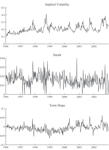
Table 1 reports the average implied volatility of the options in the sample. Rather than tabulating the option prices, we show the Black-Scholes implied volatilities since
they are easier to interpret.17We divide all options into nine buckets according to moneyness (stock price divided by the strike price) and time to maturity: moneyness less than 0.95, between 0.95 and 1.05, and above 1.05; time to maturity less than 45 days, between 45 and 90 days, and greater than 90 days. Note that when moneyness is greater than 1, the put options are out of the money. The average implied volatility across all options in our sample was 22.77%. The first panel of figure 1 plots the time series of the implied volatility of the short-term (maturity less than 45 days and as close as possible to 30 days) option with moneyness closest to
S/K ⫽ 1 (at-the-money). We can see that the implied
volatility changes substantially over time. The spike in the implied volatilities observed in fall 1998 corresponds to the Russian default crisis and long-term capital management debacle. For a fixed maturity, we can observe that the implied volatilities decrease and then increase with the strike price. This is the well-known “volatility smirk.” The second panel plots the time series of the “smirk,” defined as
16If Wednesday is not a trading day, we obtain prices from, in order of
preference, Tuesday, Thursday, Monday, or Friday.
17Here, we use the Black-Scholes model to invert option prices for
implied volatilities. This does not mean that the options are priced in the market according to that model and, indeed, we will use our model with stochastic volatility and jumps to price the options in the empirical section below. The Black-Scholes formula is used as a device to translate option prices into volatilities, which are easier to interpret.
TABLE1.—IMPLIEDVOLATILITIES OFS&P 500 INDEXOPTIONS
Moneyness
Days to Expiration
Tⱕ 45 45⬍ Tⱕ 90 T⬎ 90
S/K⬍0.95 23.83 21.39 20.7
(4.67) (4.14) (3.88)
[193] [262] [466]
0.95ⱕ S/K⬍ 1.05 20.68 20.75 21.32
(4.95) (4.62) (4.26)
[3,155] [2,928] [2,211]
S/Kⱖ1.05 27.43 25.54 24.3
(5.67) (5.22) (4.63)
[2,029] [1,924] [1,317]
Note: We report average implied volatility, the standard deviation of implied volatilities (in parenthe-ses), and the number of options (in brackets) within each moneyness-maturity bucket.
FIGURE 1.—TIME SERIES OF IMPLIED VOLATILITIES
19960 1997 1998 1999 2000 2001 2002 0.1
0.2 0.3 0.4 0.5
Implied Volatility
19960 1997 1998 1999 2000 2001 2002 0.01
0.02 0.03 0.04
Smirk
1996 1997 1998 1999 2000 2001 2002
−0.1
−0.05 0 0.05 0.1
the difference between the Black-Scholes implied volatili-ties of two short-term put options with moneyness closest to
S/K ⫽ 1.025 (out-of-the-money) and S/K ⫽ 1
(at-the-money), respectively. It shows that the smirk is positive all the time and there are changes in the steepness of the smirk over time. The third panel of figure 1 plots the time series of the “term slope,” defined as the difference between the Black-Scholes implied volatilities of the two at-the-money put options with two maturities: short term (defined as above) and long term (greater than 45 days and as close as possible to 60 days), respectively. It shows that there is some variation in the slope of the term structure through time. During our sample period, the term slope was on average close to flat.
B. Econometric Method
We adopt an implied-state quasi-maximum likelihood (IS-QML) estimation method that is similar to the implied-state generalized method of moments (IS-GMM) of Pan (2002). Our approach combines information from stock and option prices, taking advantage of the existence of an analytical option pricing formula. In Pan (2002), volatility is the only latent state variable that has to be implied. We extend Pan’s method to our setting, where both volatility and jump intensity are latent and have to be implied. We estimate the model parameters by maximizing the joint likelihood function of a discrete approximation of the con-tinuous time transition densities of the state variables and the density of the cross-sectional option pricing errors. One advantage of the QML method is that we do not need to choose the moment conditions, which is always a sensitive choice in GMM.
Our modeling of the quasi-likelihood function is inspired by Duffee (2002), who estimates a dynamic term structure model. We assume that some options are observed without error or imply the state variables, while others are observed with error. Our quasi-likelihood function combines the time series distribution of the implied state variables and the cross-sectional distribution of the pricing errors. In contrast, Pan (2002) uses only the time-series data of the implied state variables to define her moment conditions.
For estimation, we use weekly data for the stock index and four put option contracts {St,Pt
1, Pt 2, Pt 3, Pt
4}, where Pt
1
andPt
2 have the shortest maturity and Pt
3 and Pt
4 have the second shortest maturity. Pt
1 and Pt
3 are closest to at-the-money;Pt
2 and Pt
4are closest to moneyness (
S/K) of 1.05. The maturity of the first two options is greater than 15 days and as close as possible to 30 days, while the maturity of the last two options is greater than 45 days and as close as possible to 60 days.18All four contracts are actively traded.
We usePt 1and
Pt
2to imply the state variables
YtandZtand usePt
3 and Pt
4 to compute the pricing errors.
Note that the ith put option price can be expressed as
Pti ⫽ f(St, Yt, Zt; Ki, Ti, ), where f is given by equation (28) together with put-call parity,Ki and Ti are the strike price and time to maturity of theith option, and
⫽(Y,Y, Y,Z, Z,Z, Q, Q,SY, SZ, YZ,␥) is the vector of model parameters under the objective prob-ability measure. Given , proxies Yt and Zt for the
unobserved Yt and Zt can be obtained by inverting
the system of equationsPt 1⫽
f(St,Yt,Zt; K1, T1,) and
Pt 2 ⫽
f(St, Yt, Zt; K2, T2, ).19
GivenYtandZt, the model-based option pricesPt 3,and
Pt
4,for the third and fourth options can be calculated using
the option pricing formula. We then compute the Black-Scholes implied volatilities t
3, and
t
4, for these two
options based on the model prices. The measurement errors are defined as⑀ti
,⫽
t i,⫺
t
i, wherei ⫽ 3 and 4, and t i
is the Black-Scholes implied volatility of the ith option based on the observed market price. Let⑀t
⫽ 共
⑀t
4,
⑀t
3,
兲 denote the vector of measurement errors.
For week t, the log likelihood under the objective prob-ability measure is defined as
lt共 兲⫽logfX共Xt
兩X
t⫺1
兲
⫹logf⑀共⑀t
兲,
wherefX is the conditional density of the vector of state variablesXt
⫽(
St,Yt
,
Zt
)ⳕand
f⑀is the density function
of the vector of pricing errors⑀t. This specification
implic-itly assumes that the pricing errors are independent of the state variables.
Generalizing the approach of Ball and Torous (1983), we use the truncated Poisson-normal mixture distribution to approximatefXfor the jump-diffusion model in equations (1) to (3). Let ⌬t be the time interval of discretization, which is 1/52 for our weekly frequency data. We approxi-mate equations (1) to (3) by the following discrete system:
⌬lnSt⫽共r⫹t⫺1⫺t⫺1Q兲⌬t⫹Yt⫺1
冑
⌬t⑀S,t⫹QtBt (32)⌬Yt⫽共Y⫹YYt⫺1兲⌬t⫹Y
冑
⌬t ⑀Y,t (33)⌬Zt⫽共Z⫹ZZt⫺1兲⌬t⫹Z
冑
⌬t ⑀Z,t, (34)where (⑀S,t, ⑀Y,t, ⑀Z,t) ⬃ i.i.d. ᏺ(0, ⌺), Qt ⬃ i.i.d. ᏺ(Q,
Q 2),
Qt and ⑀t are independent, Bt ⬃ i.i.d. ᏼˆ(t⫺1⌬t) whereᏼˆis the truncated Poisson distribution with
trun-cation taken atM, the maximum number of jumps that may
occur during a time interval.20We fixMto be 5 in our paper.
18Using two maturities helps in identifyingY andZ since jumps and
stochastic volatility have different effects on short- and long-term options. We are constrained in using options with longer maturities than a few months since they are not liquid. The results are robust to choosing options with moneyness 0.95, 0.975, or 1.025.
19It is not always the case thatYandZcan be inverted for a given vector
of parameters. The intuition is that bivariate quadratic equations do not always have real solutions. We impose the constraint that the vector of parametersallows inversion ofYandZ.
Our discrete model, equations (32) to (34), allows multiple (up toM) jumps in a time interval, while Ball and Torous (1983) consider at most only one jump during a time interval. We approximatefXby the likelihood function of equations (32) to (34), which is a mixture of truncated Poisson and normal distributions.21We examine the preci-sion of the approximation in the online appendix.
To model f⑀, we assume that the option pricing error
vector ⑀t has an i.i.d. bivariate normal distribution with constant covariance matrix. Given the definition of the log-likelihood functionlt(), the QML parameter vector is obtained from the optimization program:
max
L共 兲⫽max
t
冘
⫽1T
lt共 兲.
We employ an optimization algorithm similar to that of Duffee (2002). In step 1, we generate starting values for the parameter vector. In step 2, we use the formula (28) and option pricesPt
1, Pt
2to derive the implied state variables Yt andZt. In step 3, we use the nonlinear Simplex algorithm to obtain a new parameter vector that improves the QML value. We then repeat the above steps until convergence is achieved. The standard errors of the parameter estimates are obtained from the last QML optimization step. The estima-tion time for the SV-SJ model ranges from two to four hours depending on the choice of the initial parameter values.
In addition to the general model (SV-SJ), we also esti-mate two restricted cases: the stochastic volatility model (SV) and the constant jump intensity model (SV-J). For the restricted models, volatility is the only latent state variable that needs to be implied. Therefore, in those cases, we invert just the short-term at-the-money optionPt
1to imply the state variableYt.
It is important to point out that the options are priced under the risk-adjusted probability measure, while the tran-sition densities of the state variables are specified under the objective probability measure. The fact that the likelihood function combines information from both the objective and the risk-adjusted distribution of the state variables has a crucial role in the estimation of the risk-aversion parameter
␥. A necessary identification condition is that the transfor-mation between the objective and the risk-adjusted
proba-bility measure be monotonic in terms of ␥. In our
frame-work, this transformation is given by equations (22) to (27),
which depends on ␥. For the SV model, the difference
between *YY andY is⫺␥SYY, which is clearly mono-tonic in␥.22For the SV-SJ model, the difference between
*YY and Y is more complex but can still be shown to be
monotonic in ␥ using the parameter estimates reported in
table 2. Intuitively, the identification of␥ comes from the mean reversion speed observed in the implied state vari-ables, coupled with the mean reversion speed implicit in the
option prices. The mean reversion speeds ofYandZunder
the objective probability measure enter the likelihood func-tion through the transifunc-tion density fX(Xt兩Xt⫺1), while the same coefficients under the risk-neutral probability measure enter the likelihood function through the density of the pricing errorsf⑀(⑀t). Since the transformation between the mean reversion speeds under the two probability measures
is monotonic, the QML algorithm finds a unique value of␥
that maximizes the combined likelihood function.23 The
precision of the estimate of ␥ is remarkable and much
greater than could be achieved by estimating this parameter from the drift of the stock market alone.
Another potential problem in our QML approach is that the approximation of the conditional likelihood function
fX by the truncated Poisson-normal mixture distribution may bias the estimates of the model parameters. In the online appendix, we conduct Monte Carlo simulations to verify the precision of the approximation. We show that the QML estimates are close to the true parameters (used for the simulations) indicating no significant bias in our estimation approach.
21It is well known that the log-likelihood function for a mixture of
normal distributions is unbounded, but it is still possible to obtain consistent and asymptotically normal distributed estimates by constraining the maximum likelihood algorithm (see, for example, Hamilton, 1994).
22In some studies of the SV models⫺␥
SYYis called the market price
of risk. Using the parameter estimates reported in table 2, this market price
of risk is positive. 23We thank an anonymous referee for this explanation.
TABLE2.—ESTIMATEDPARAMETERS
SV SV-J SV-SJ
Y 1.929 1.756 2.841
(0.340) (0.314) (0.346)
Y ⫺9.201 ⫺9.218 ⫺18.079
(1.541) (1.545) (2.065)
Y 0.306 0.315 0.334
(0.008) (0.009) (0.010)
Z 7.745
(1.396)
Z ⫺9.436
(1.567)
Z 1.529
(0.045)
Q ⫺0.070 ⫺0.098
(0.012) (0.013)
Q 0.283 0.160
(0.013) (0.013)
SY ⫺0.731 ⫺0.728 ⫺0.495
(0.014) (0.014) (0.025)
SZ ⫺0.597
(0.022)
YZ 0.168
(0.045)
␥ 1.977 1.984 1.917
(0.391) (0.369) (0.352)
RMSE(%) 3.348 2.730 2.131
IV. Empirical Results
In this section we discuss the empirical results. We present the model estimates and discuss the performance of the model in pricing options.
A. Model Estimates
The SV-SJ model of stochastic volatility and stochastic jump intensity contains the pure stochastic volatility model (SV) and the constant jump intensity model (SV-J) as
special cases. In the SV model, we restrict Q ⫽ Q ⫽
Z⫽ Z⫽ SZ⫽ YZ ⫽0. In the SV-J model, we restrict
Z ⫽ Z ⫽ SZ ⫽ YZ ⫽ 0, and t ⫽ is a constant.24 Table 2 reports the estimated parameters for the three models. We can compare to some extent the parameter estimates for the SV model with the estimates reported by Bakshi, Cao, and Chen (1997) and Pan (2002). However, notice that their SV model is the square root model of Heston (1993), whereas ours is similar to the model of Stein and Stein (1991). Also, their sample periods are different from ours. Bakshi et al. use S&P 500 index options data from 1988 to 1991, and Pan uses S&P 500 index options data from 1989 to 1996.
In Bakshi et al. (1997) and Pan (2002), the square root of the
estimated long-run mean of Vis 18.7% and 11.7%,
respec-tively. Our estimate of the long-run mean of公V(⫽兩Y兩), given by Y/Y, is a bit higher, at 21.0%. These differences are mainly due to the difference in sample periods. The estimates of mean-reversion speed are 1.15 and 7.10 in their papers, whereas it is 9.20 in our paper, implying stronger mean reversion.25The volatility of volatility is 0.39 and 0.32 in their
papers, and it is 0.31 in our paper.26The correlation between the stock and volatility processes is estimated to be⫺0.64 and
⫺0.57 in their papers, and it is⫺0.73 in our paper.
Bakshi et al. (1997) and Pan (2002) also estimate an SV-J model. In this case, the square root of their estimated
long-run mean of V is 18.7% and 11.6% in their papers,
whereas our estimate is 19.0%. The mean-reversion speed is estimated as 0.98 and 7.10 in their papers and 9.22 in our paper. The volatility of volatility is 0.42 and 0.28 in their papers and 0.31 in our estimate. The correlation between volatility and the stock is⫺0.76 and⫺0.52 in their papers
and ⫺0.73 in ours. Finally, they estimate the mean jump
size to be ⫺5 percent and ⫺0.3 percent, respectively,
whereas we estimate it to be⫺7 percent. In summary, our
estimates for the restricted SV and SV-J models are com-parable with the findings in other studies despite the differ-ences in the data sets and models.
We next concentrate our attention on the SV-SJ model. All the coefficients of the model are significant at any conventional level of significance. Table 3 reports summary statistics for the implied time series of公Vtandt, which are plotted in figure 2.
The average level of volatility is 15.6%, and the average level of jump intensity—loosely speaking, the expected number of jumps over the next year—is 0.80. The average
jump size is⫺9.8%, which is 40% higher than the average
jump size in the SV-J model.
Both the volatility and jump intensity series exhibit sub-stantial variation through time. The diffusive volatility var-ies between 1.9% and 35.6%. The jump intensity varvar-ies from less than 0.01 to over 5 during the 1998 financial crisis. Interestingly the two risk sources, although corre-lated, can display very different behavior: from times of high diffusive and jump risks, as in the second half of 2002; 24Note that option pricing formula for the SV-J model cannot be
obtained from that of the SV-SJ model by restricting the corresponding parameters. A similar option pricing formula can be derived using the same approach as for the SV-SJ model.
25Our estimate of mean reversion speed is much faster than those of
some early studies. One explanation is that previous studies generally use an early sample period. As a check, we examined the at-the-money nearest-to-maturity implied volatility for the period 1990–1995 (from CBOE data since Option Metrics is not available for that period). The first-order autocorrelation coefficients are 0.911 and 0.822 for the 1990–
1995 and 1996–2002 periods, respectively, indicating faster mean rever-sion in the more recent period.
26According to Ito’s lemma, the volatility of volatility in Heston’s model
is half that in our model. So our estimate of volatility of volatility is about twice of those in Bakshi et al. (1997) and Pan (2002). But this higher volatility is offset by a much faster rate of mean reversion.
TABLE3.—IMPLIEDDIFFUSIVEVOLATILITY ANDJUMPINTENSITY
Model Mean S.D. Skewness Kurtosis Maximum Minimum Autocorrelation Corr (公Vt,t)
SV 公Vt 0.207 0.075 1.013 4.531 0.540 0.067 0.822
t
SV-J 公Vt 0.188 0.077 0.943 4.416 0.520 0.034 0.821
t 0.143
SV-SJ 公Vt 0.156 0.061 0.446 3.174 0.356 0.019 0.656 0.583
t 0.795 0.714 2.061 9.188 5.240 0.000 0.795
J-B Q1 Q5 Q10
⑀Y 13.298 12.061 34.530 56.227
(0.001) (0.001) (0.000) (0.000)
⑀Z 29.904 9.631 18.283 25.528
(0.000) (0.002) (0.003) (0.004)
to times when jump risk is high but diffusive risk is low, as in the fall of 1998; to times when both risks are low, as in the beginning of 1996.
The implied time series of volatility from the SV-SJ model is different from those of the other two models. The average implied volatility, 15.6%, is much lower in the SV-SJ model than in the SV model since the stochastic volatility in the latter model needs to account for all the risk, including the jump risk.
The estimated volatility process in the SV-SJ model is mean reverting at about twice the speed as in the SV and SV-J models. The implied time series of stochastic volatility and jump intensity show autocorrelations of 0.66 and 0.79, respectively.
The estimated correlation between the increments of the diffusive volatility and jump intensity is quite low, at 0.17. This is evidence that the two processes are largely uncor-related and do not support models that make jump intensity vary with the level of diffusive volatility. Increments of the diffusive volatility are negatively correlated with stock
returns, ⫺0.50, which is smaller than that in the SV and
SV-J models. Changes in jump intensity are also negatively correlated with stock returns at a higher absolute value,
⫺0.60.
Overall, our results are also consistent with the recent literature on multifactor variance models (Alizadeh, Brandt, & Diebold, 2002; Chacko & Viceira, 2003; Chernov et al., 2002; Engle & Lee, 1999; Ghysels, Santa-Clara, & Val-kanov, 2005), which finds reliable support for the existence of two factors driving the conditional variance. The first factor is found to have high persistence and low volatility,
whereas the second factor is transitory and highly volatile. The evidence from estimating jump diffusions with stochas-tic volatility points in a similar direction (Jorion, 1988; Anderson, Benzoni, & Lund, 2002; Chernov et al., 2002; Eraker et al., 2003). For example, Chernov et al. (2002) show that the diffusive component is highly persistent and has low variance, whereas the jump component is by as-sumption not persistent and is highly variable.
The second panel of table 3 reports Jarque-Bera and Ljung-Box statistics for the innovations of the state variablesYandZ. The Jarque-Bera statistics are significant, indicating nonnor-mality of the innovations. The Ljung-Box statistics are also significant, implying serial correlation in the innovations. Both diagnostic tests indicate misspecification of the SV-SJ model. Pan (2002) also finds that her jump-diffusion model is mis-specified. Since her model is similar to the SV-J model in our paper, the sources of misspecification are likely to be similar. Pan argues that the misspecification shows evidence of jumps in volatility, as modeled in Duffie et al. (2000) and empirically studied in Eraker et al. (2003).
B. Option Pricing Performance
We evaluate the option pricing performance of the model in terms of the root mean squared error (RMSE) of Black-Scholes implied volatilities. The implied volatility error of a given option is the difference between the implied volatili-ties calculated from market price and model price. Allowing the jump intensity to vary stochastically proves to be quite important for options pricing. As reported in the last row of table 2, the RMSE of the SV-SJ model for all options in our
data set is 2.13%, measured in units of implied volatility. This is smaller than the RMSEs of the SV and SV-J models, which are 3.35% and 2.73%, respectively. Standardt-tests show that the RMSEs are significantly different from each other. For example, the t-statistic for a difference between the SV-J and SV-SJ models is 14.75. Despite the improve-ment in fitting the option prices, significant pricing errors remain as the RMSE of the SV-SJ model is still about twice the average bid-ask spread in our sample, which is 1.01% (with a standard deviation of 0.66%), again in units of Black-Scholes implied volatility.
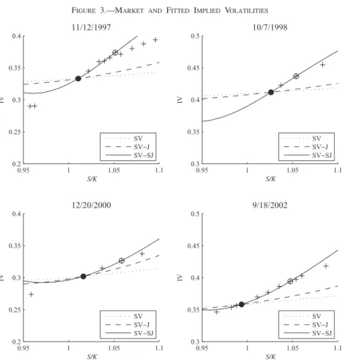
Figure 3 plots the market-implied volatilities of options with the shortest maturity, together with the fitted implied volatilities of the three alternative pricing models in four different dates of the sample. We find that the SV-SJ model does a much better job at pricing the cross-section of options than the other two models for these four days when the implied volatilities are high.
Having established that our model can effectively capture the time-series and cross-section properties of option prices, we now try to improve our understanding of the model. In particular, we want to understand the relative roles of the diffusive volatility and jump intensity in pricing options. Figure 4 shows the plots of implied volatility smiles at
different maturities produced by our model, using the esti-mated parameters and different values of volatility and jump intensity. In the first two cases, the diffusive volatility,公V, is fixed at its sample average while the state variable for
jump intensity, Z, is either at its sample average or 1
standard deviation above or below it. In the next two cases, the state variable for jump intensity,Z, is fixed at its sample average, while the diffusive volatility,公V, is either at its sample average or 1 standard deviation above or below it. The time to maturity is either 30 days or 90 days. We find that both volatility and jump intensity have an impact on the level of implied volatilities. Further-more, the persistence in both risk components guarantees that their effects are felt at long horizons. But the two state variables have different impacts on the shape of the implied volatility smile. Jump intensity has a large im-pact on the prices of all short-term options but it affects
out-of-the-money puts (high S/K) more than
in-the-money puts (low S/K). The volatility has a larger
impact on the prices of near-the-money options than those of away-from-the-money options. The longer the maturity, the flatter the volatility smiles, reflecting mean reversion in the volatility and jump intensity processes. The differential impact of volatility and jump intensity on
FIGURE 3.—MARKET AND FITTED IMPLIED VOLATILITIES
0.95 1 1.05 1.1
0.2 0.25 0.3 0.35 0.4
11/12/1997
S/K
IV
SV SV−J SV−SJ
0.95 1 1.05 1.1
0.3 0.35 0.4 0.45 0.5
10/7/1998
S/K
IV
SV SV−J SV−SJ
0.95 1 1.05 1.1
0.2 0.25 0.3 0.35 0.4
12/20/2000
S/K
IV
SV SV−J SV−SJ
0.95 1 1.05 1.1
0.3 0.35 0.4 0.45 0.5
9/18/2002
S/K
IV
SV SV−J SV−SJ
options of varying maturity and moneyness is what al-lows us to identify the two state variables in the estima-tion.
V. Option-Implied Risks and the Equity Premium
In this section we study the equilibrium equity premium implied by the parameter estimates and the implied state variables.
A. The Equity Premium
The estimate of␥in table 2 for the SV-SJ model is 1.917, which seems quite reasonable. In an economy without jumps and with constant volatility, Merton (1973) shows that the equity premium demanded by an investor who holds the stock market is equal to␥times the market’s variance. Since the realized volatility in our sample was 18.8%, using the estimated risk aversion coefficient, we obtain an
uncon-ditional equity premium of 6.8% (1.917 ⫻ 0.1882). This
premium approximately matches the historic average excess stock market return of between 4% and 9% (depending on the sample period) reported by Mehra and Prescott (2003). Note that we are studying the portfolio choice of an investor who derives utility from next period’s wealth, not utility from lifetime consumption. In the latter case, it is well
known from Mehra and Prescott (1985) and much subse-quent work that a much higher level of risk aversion is needed to match the historic equity premium.
In what follows, we keep the horizon of the representative
investor at 1 month, T ⫽ 1/12.27 The choice of a short
horizon abstracts away from hedging demands, making the interpretation of the results simpler.28Given the relatively strong mean reversion in the risk processes, it is unlikely that horizons longer than one month would generate hedg-ing demands strong enough to change the results.29
27The results are robust to this choice of time horizon. We triedTfor up
to ten years, and the main results do not change quantitatively. All the coefficients ofB andCconverge quickly to a limit asT increases, and after one month, they are virtually constant. Moreover, these coefficients are small in magnitude. Their impact on the equity premium is corre-spondingly small. The component of the equity premium that involvesB
andCis generally negative with small magnitude (bounded by 2% and on average less than 0.5%) in comparison to the average size of the equity premium, which is over 10%. It is reasonable to say thatBandCare not critical in determining the size and variation of the implied equity premium that we find.
28Note that we are considering preferences for terminal consumption. A
given horizon in our model should be compared with the “duration” of utility in a model with intermediate consumption (which is necessarily less than the terminal date).
29Chacko and Viceira (2005) find that the hedging demands induced by
stochastic volatility are tiny due to the strong mean reversion. FIGURE 4.—VOLATILITY SMILE OF THE SV-SJ MODEL
0.9 0.95 1 1.05 1.1 0.1
0.15 0.2 0.25 0.3
λ=0.659, T=30
S/K
IV
V1/2=0.217 V1/2=0.156 V1/2=0.095
0.9 0.95 1 1.05 1.1 0.1
0.15 0.2 0.25 0.3
λ=0.659, T=90
S/K
IV
V1/2=0.217 V1/2=0.156 V1/2=0.095 0.9 0.95 1 1.05 1.1
0.1 0.15 0.2 0.25 0.3
V1/2=0.156, T=30
S/K
IV
λ=1.394
λ=0.659
λ=0.196
0.9 0.95 1 1.05 1.1 0.1
0.15 0.2 0.25 0.3
V1/2=0.156, T=90
S/K
IV
λ=1.394
λ=0.659
λ=0.196
Note: The four panels show the plots of the Black-Scholes implied volatility smiles at different maturities produced by the SV-SJ model, using the estimated parameters reported in table 2 and for different values of volatility (公V) and jump intensity (). In the top two panels,公Vis fixed at its sample average (0.156) while(⫽Z2) is chosen so thatZis at its sample average and that value plus or minus one standard
Equation (13) gives us the equity premium as a function of the diffusive volatility and jump intensity. With the estimated parameters of the model, we can evaluate the coefficients of that function:
⫽1.917Y2
⫺0.008Y⫺0.009Y2
(35)
⫺0.022YZ⫹0.087Z2.
Given the implied series of the diffusive volatility Y and jump intensityZ, we can compute the average of the equity premium in our sample. This gives us an estimate of the unconditional equity premium of 11.8%. Note that this is different from putting the average level of the implied series of the diffusive and jump risks in the above equation because of the nonlinearity of the equity premium inYand
Z. Note also that this calculation does not match the average excess return of the S&P 500 index in our sample, which is only 2%. The reason is that we did not use stock returns in the calculation, only the measures of risk implied from option prices together with the estimated level of risk aversion.
Remember that the premium demanded by an investor with the same preferences in an economy without jumps and with constant volatility was 6.8%. Therefore, the uncondi-tional equity premium we computed with the risk inferred from option prices is more than 70% higher than the premium for realized risk.30
These findings have some bearing on the discussion of the equity premium puzzle first investigated by Mehra and Prescott (1985) and recently surveyed in Mehra and Prescott (2003). The equity premium puzzle is typically stated as the historic average stock market return far exceeding the com-pensation for its risk that would be required by an investor with a reasonable level of risk aversion. It should be noted that the literature on the equity premium puzzle usually measures risk by the covariance of stock market returns with aggregate consumption growth. However, none of our calculations involves consumption, and there is no way we can obtain the implied covariances between stock market returns and consumption growth from option prices. What we do show is that the risk premium demanded by an investor with utility for wealth living in an economy with the realized level of market volatility is only slightly more than half the premium demanded by the same investor when taking into account the risks assessed by option markets.
The puzzle is that the historic stock market premium of, say, 6%, is much higher than the approximately 1% excess return warranted by the covariance of the stock market returns with consumption growth (for reasonable levels of
risk aversion). Our point is that the realized covariance of the stock market returns with consumption growth is likely to understate the true risk of the market by as much as the realized volatility understates the risk implicit in option prices. In our simple calculation above, we found that the ex ante risk premium almost doubles when we use the option implied risks instead of the realized volatility. If the same factor were to apply to the consumption-based risk measure, the equity premium puzzle would be considerably less-ened.31
These results confirm a substantial peso problem when measuring the riskiness of the stock market with realized volatility. The risks investors perceive ex ante and that are therefore embedded in option prices far exceed the realized variation in stock market returns.
If investors price the stock market to deliver returns that compensate them for the perceived level of risk, the equity premium can easily be twice what is justifiable from the level of realized risk. This is the fundamental idea of Brown et al. (1995): ex post measured returns include a premium for some bad states of the world that investors deemed probable but did not materialize in the sample. Similarly, Rietz (1988) proposed a solution for the equity premium puzzle based on a very small probability (about 1%) of a very large drop in consumption (25%). That is not far from the risks perceived by investors in the option market. Barro (2006) extended the analysis of Rietz to show that rare events can explain a variety of asset pricing regularities. Goetzmann and Jorion (1999) provide empirical evidence that large jumps have occurred in a variety of countries in the twentieth century and that the United States was an outlier, with both few crashes and the highest realized average return.
Of course, this discussion only shifts the equity premium puzzle to a puzzlingly large difference between the level of perceived risk and the level of realized risk: the option market predicted a lot more market crashes than the number that actually occurred. For example, given the average jump size and average intensity estimated in tables 2 and 3, the stock market should experience market crashes with a
magnitude of ⫺9.8% once every 1.26 years. This is
obvi-ously very different from the observed frequency and mag-nitude of stock market jumps. The interesting finding is that the puzzlingly high risks implicit in option markets match the puzzlingly high equity premium for very reasonable preferences.
B. Time Variation in the Equity Premium
The previous section discussed the unconditional equity premium. We now discuss the time variation in the equity premium. Figure 5 plots the time series of the risk premium 30The high equity premium obtained here may be caused by our choice
of the sample period, which was much more volatile than other periods (1990–1996). It may also be partially driven by our specific option pricing model. As options may contain high premia, they can be translated into high premia in the stock returns. We thank an anonymous referee for pointing this out.
31Especially if we consider the estimates of the equity premium of