COMPARING CONDITIONAL AND STOCHASTIC
VOLATILITY MODELS: GOODNESS OF FIT,
FORECASTING AND VALUE-AT-RISK
COMPARING CONDITIONAL AND STOCHASTIC
VOLATILITY MODELS: GOODNESS OF FIT,
FORECASTING AND VALUE-AT-RISK
Disserta¸c˜ao apresentada ao
Departamento de Estat´ıstica da UFMG
como requisito parcial para a obten¸c˜ao
do t´ıtulo de Mestre em Estat´ıstica.
Advisor: Thiago Rezende dos Santos
Co-advisor: Frank Magalh˜aes de Pinho
Primeiramente agrade¸co ao meu orientador Thiago e ao meu co-orientador Frank, cujo apoio e paciˆencia foram cruciais nessa jornada e sem os quais esse trabalho n˜ao seria poss´ıvel. Agrade¸co
tamb´em ao Ivair e `a Glaura pela leitura cuidadosa do manuscrito e pelos coment´arios e
re-comenda¸c˜oes feitas para a melhora do trabalho.
Agrade¸co profundamente `a toda minha fam´ılia, em especial `a minha m˜ae Maria Bernadete, ao meu pai Evandro e `a minha noiva Alice; o amor e suporte de vocˆes ´e o fundamento da minha vida. Serei sempre grato ao meu irm˜ao Glauco, grande companheiro e enorme influˆencia em mim tanto como pessoa quanto como profissional.
No departamento de Estat´ıstica da UFMG, onde esse trabalho de mestrado foi realizado,
agrade¸co profundamente `a todos os meus professores e colegas pelo acolhimento, companheirismo
e pelas sempre agrad´aveis discuss˜oes e conversas. Agrade¸co tamb´em aos meus professores e colegas de gradua¸c˜ao da Economia no Ibmec MG, com os quais aprendi tanto e fui inspirado `a fazer parte do meio acadˆemico.
Finalmente, agrade¸co aos meus outros amigos e a todas `as pessoas que de alguma forma
con-tribu´ıram para a produ¸c˜ao desse trabalho e da minha forma¸c˜ao. N˜ao citarei nomes por receio de omitir algu´em.
A produ¸c˜ao desse trabalho e meu mestrado foram totalmente financiados pela CAPES, `a qual
dedico um agradecimento especial. O desenvolvimento e divulga¸c˜ao de minha pesquisa foram
Nesse trabalho uma compara¸c˜ao das trˆes fam´ılias de volatilidade Autoregressive Conditional Heteroskedasticity(ARCH),Stochastic Volatility(SV) eNon-Gaussian State Space Models(NGSSM) ´e feita de acordo com trˆes diferentes m´etricas: ajuste, previs˜ao eValue-at-Risk (VaR). Procedi-mentos de inferˆencia sobre a distribui¸c˜ao Skew Generalized Error s˜ao detalhados. Os respectivos crit´erios de avalia¸c˜ao usados para cada m´etrica s˜ao o Crit´erio de Informa¸c˜ao de Akaike, Erro Quadr´atico M´edio das previs˜oes um passo `a frente e Cobertura Incondicional do VaR um passo `a frente. A amostra utilizada ´e composta por s´eries de retornos di´arios (Ibovespa, Hang Seng Index, Merval Index e S&PTSX Index) de Janeiro de 2000 at´e Janeiro de 2016 ou 4000 observa¸c˜oes, das quais 3000 s˜ao utilizadas para estima¸c˜ao e 1000 s˜ao reservadas para previs˜ao e avalia¸c˜ao do VaR.
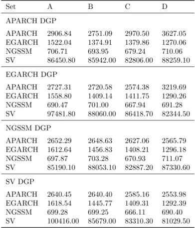
As estimativas obtidas servem de base para a condu¸c˜ao de um experimento de simula¸c˜ao
envol-vendo 1000 replica¸c˜oes de s´eries com o mesmo n´umero de observa¸c˜oes para estima¸c˜ao e previs˜ao dos dados de retorno.
Resultados das simula¸c˜oes indicam que o modelo SV apresenta consistentemente o melhor
de-sempenho quanto ao ajuste e previs˜ao, ficando atr´as apenas do APARCH na avalia¸c˜ao do VaR um
passo `a frente. Conclus˜oes para o EGARCH e o NGSSM s˜ao mistas: quanto ao ajuste, o APARCH
fica em segundo, o NGSSM em terceiro e o EGARCH em ´ultimo; quanto `a previs˜ao, o EGARCH
fica em segundo, o APARCH em terceiro e o NGSSM em ´ultimo; quanto ao VaR, o APARCH fica
em primeiro, o EGARCH em terceiro e o NGSSM em ´ultimo. O tempo de CPU gasto na estima¸c˜ao
de cada modelo tamb´em ´e reportado e comparado: tomando o NGSSM como base, a estima¸c˜ao
do modelo SV demora 82 vezes mais, enquanto a estima¸c˜ao do APARCH demora 4 vezes mais e o
EGARCH 2 vezes mais.
Palavras-chave: Heterocedasticidade Condicional, Modelos de Espa¸cos de Estados N˜ao-Gaussianos,
In this work a comparison of three families of volatility models, namely the Autoregressive Conditional Heteroskedasticity (ARCH), Stochastic Volatility (SV) and Non-Gaussian State Space Models (NGSSM) is made according to three different metrics: goodness of fit, forecasting and assessing Value-at-Risk (VaR). Inference procedures under the flexible Skew Generalized Error family of distributions is detailed. Respective evaluation criteria used for these metrics are the Akaike Information Criterion, Mean Squared Error of one-step-ahead forecasts and Unconditional Coverage of one-step-ahead VaR. The data used are daily asset return series (Ibovespa, Hang Seng Index, Merval Index and S&PTSX Index) from Jan-2000 to Jan-2016, or roughly 4000 observations, from which 3000 are used for estimation and 1000 are reserved for forecasting and VaR evaluation. Parameter estimates serve as basis to conduct a simulation experiment which consists of 1000 replications of series with the same number of observations for estimation and forecasting as the return data.
Simulation results indicate that the Stochastic Volatility model consistently outperforms com-peting specifications in goodness of fit and forecasting, and ranks second (right after the APARCH) in assessing the out-of-sample VaR. Conclusions for the EGARCH and NGSSM are mixed: in good-ness of fit performance, the APARCH ranks second, the NGSSM ranks third and the EGARCH ranks last; in forecasting performance, the EGARCH is second, the APARCH third and the NGSSM last; in VaR assessment, the APARCH ranks first, the EGARCH third and the NGSSM last. CPU time spent on the estimation of each model is also reported and compared: taking the NGSSM as the benchmark, estimation of the SV model takes about 82 times as long, while APARCH estima-tion takes about 4 times and EGARCH estimaestima-tion about 2 times.
1 INTRODUCTION 1
2 VOLATILITY MODELS 3
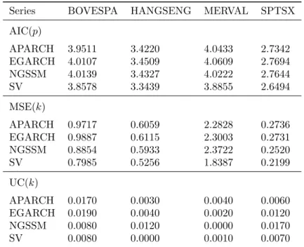
2.1 Model Evaluation Criteria . . . 5
2.2 Autoregressive Conditional Heteroskedasticity . . . 7
2.3 Stochastic Volatility . . . 9
2.4 Non-Gaussian State Space Models . . . 14
3 APPLICATION 16
4 SIMULATION EXPERIMENT 23
5 CONCLUSION 27
1. INTRODUCTION
Volatility plays a key role in Finance, representing the risk of an asset. It is therefore the basis for risk management, portfolio optimization, assessing the Value-at-Risk, and the pricing of options, futures and derivatives. Volatility is also important in Economics, where risk-averse agents will require premia for more volatile operations, and where it can also be used as a measure of how agents’ decisions and preferences change over time, or even to assess the non-constant variability of economic variables such as output, money supply and inflation.
Performing statistical inference for the volatility is an issue that has received special attention. Since volatility is non-observable, estimating it requires a specific set of techniques. Engle (1982) proposed a conditioning argument that solves the problem for deterministic volatility dynamics. Specifically, in his Autoregressive Conditional Heteroskedasticity (ARCH) model, volatility is a function of past squared values of the original time series. Therefore, by conditioning on the immediate past information set, volatility is effectively an observable quantity. Later, Bollerslev (1986) proposed the Generalized ARCH (GARCH) model, in which the volatility is also allowed to depend on its own past, analogously to an Autoregressive Moving Average (ARMA) model. However, the GARCH specification is limited; according to Carnero et al. (2004), GARCH models require additional distribution assumptions and parameter values that make the model close to nonstationary in order to reproduce the behavior in daily series of financial returns.
An alternative to ARCH-type models is the Stochastic Volatility (SV) family of models, of which the first was proposed by Taylor (1982) as a first-order stochastic autoregressive process for the volatility. SV models offer a natural economic interpretation of volatility and are easier to connect with continuous-time diffusion models, which are often used in financial theory to represent the behaviour of financial returns. They are also found to be more flexible than ARCH-type models; Carnero et al. (2004) show that the basic SV model is more appropriate than the GARCH model in reproducing main empirical properties of daily returns. Another advantage is that statistical properties of SV models are simpler to derive when compared to models from the ARCH family, using elementary properties of stochastic processes.
However, the Stochastic Volatility family has a serious drawback: estimation techniques for its models are much more complicated than for ARCH models, even for the canonical autoregressive model with Gaussian innovations of Taylor (1982). There is a whole body of literature dedicated to the estimation of SV models, which is reviewed extensively in the paper by Broto and Ruiz (2004) and in the book by Bauwens et al. (2012).
An interesting alternative to both SV and ARCH-type models is the Non-Gaussian State Space Models (NGSSM) family proposed by Gamerman et al. (2013). The NGSSM in the volatility context is essentially a local scale model (a multiplicative local level model) where the dynamic level has a Beta evolution. This evolution may seem restrictive at first, but it allows for exact likelihood inference, filtering and smoothing; furthermore, observations are allowed to follow a whole plethora of distributions as long as they can be written in a specific form. Examples of distributions nested within the NGSSM family include the Normal, Laplace, Rayleigh, Poisson, Weibull and Generalized Gamma, as well as the heavy-tailed distributions included in the extension by Pinho et al. (2016), such as the Frechet, Levy, Log-gamma, Log-normal and Skew-Generalized Error Distribution (Skew-GED).
since the marginal likelihood of hyperparameters is available in closed form. Therefore, the NGSSM family seems to capture advantages of both SV and ARCH models: it allows for flexible speci-fications, but it is also computationally simple. Furthermore, when compared to the traditional lognormal SV model by Taylor (1982) and the GARCH model by Bollerslev (1986), both of which have 3 parameters, the corresponding Gaussian NGSSM only has 1 parameter to be estimated.
However, due to the fact that the NGSSM family is relatively recent, there have been few comparison studies between these three families. The works of Pinho and Santos (2013) and Pinho et al. (2016) suggest that the NGSSM family performs better than the ARCH and even than the SV model for the series taken into account. In detail, Pinho and Santos (2013) compare the fit of NGSSM (assuming various distributions) and the Asymmetric Power ARCH (APARCH) model of Ding et al. (1993) for series of daily returns of financial indexes. Their conclusion is that NGSSM outperforms APARCH when goodness-of-fit is evaluated using both Akaike and Bayesian Information Criteria (AIC and BIC, respectively) and loglikelihood values.
The work of Pinho et al. (2016) proceeds further comparing fit and forecasting performance of NGSSM, GARCH, Exponential GARCH (EGARCH) [Nelson (1991)] and log-t Stochastic Volatility also for series of daily returns of financial indexes. They conclude that the NGSSM outperforms the GARCH, EGARCH and log-t SV in fit by means of the AIC, BIC and loglikelihood and also in forecasting by means of the Square Root of Mean Squared Error (SQRMSE), calculated for 5 pseudo-out-of-sample one-step ahead forecasts.
Most of the literature on volatility models consists of new proposals along with a limited com-parison between the new model and a few already established others. Examples include Chan and Gray (2006), which introduce the AR-GARCH-EVT model and compares it with parametric and nonparametric VaR approaches in a forecasting and conditional/unconditional coverage context using electricity return data; Omori et al. (2007), which extend the MCMC-based estimation ap-proach proposed by Kim et al. (1998) to allow for a leverage effect and compares it to competing SV specifications on the basis of the marginal likelihood using japanese stock return data and De-schamps (2011), which introduces a new version of the local scale model of Shephard (1994a) and compares it with t-GARCH and lognormal SV models by means of Bayes factors using exchange rate and stock return data.
However, some papers that exclusively concern themselves with comparing models from dif-ferent families can also be found. In a forecasting context, examples include Hansen and Lunde (2005), which compare a variety of ARCH-type models by means of tests for Superior Predic-tive Ability and Reality Check for data snooping using daily exchange rate and intraday stock return data and Iltuzer and Tas (2013), which compare naive volatility estimation approaches with ARCH-type and SV models on the basis of Superior Predictive Ability, Reality Check and Model Confidence Set in different forecast horizons using stock return data.
In a Value-at-Risk context, examples include So and Yu (2006), which compare ARCH-type models by assessing VaR estimation accuracy at various confidence levels on long and short posi-tions using stock return and exchange rate data and Angelidis et al. (2004), which also compare ARCH-type models for stock return data, but assessing one-step-ahead VaR forecasts.
Finally, in the goodness of fit context, examples include Nakajima (2012), which compares SV and ARCH models by means of the marginal likelihood using daily individual securities, stock return and exchange rate data and Silva et al. (2015), which compares ARCH models on the basis of the Akaike Information Criterion using daily stock return data.
not suggest a clear prevalence of any family of models, even if the interest is limited to one specific criterion. This work is expected to fill in this suggested gap in the literature, providing relevant empirical results and an extensive simulation experiment specifically designed for the comparison of the most utilized volatility models in practice so far. Another important point of interest to the applied use of these models is a comparison of computational time, especially in financial markets, where the number of assets in a portfolio tend to be very large.
The objectives of this work are summarized below, in no particular order.
1. Provide an accessible reference for the properties and inference techniques for the families of models presented here, specifically when a skewed and leptokurtic distribution (such as the Skew-GED) is assumed for the error terms.
2. Determine a family of models as being the most adequate for each metric: goodness of fit, forecasting and Value-at-Risk.
3. Draw conclusions about which features/stylized facts influence model performance the most, overall and for each criteria.
4. Establish a trade-off between accuracy and computational efficiency between models.
The next section details the relevant volatility families and their respective inference procedures, as well as important stylized facts of financial data and respective model evaluation criteria.
2. VOLATILITY MODELS
Consider a stochastic process{Xt}∞t=0 with conditional meanE(Xt|Ψt−1), in whichEdenotes
the expectation operator and Ψt= (X0, x1, . . . , xt)′ is the information set ofXt, withX0denoting
previously available information about the process andxtdenoting a realization of Xt. Volatility
models are commonly written as a product of two independent stochastic processes, such as
xt−E(Xt|Ψt−1) =yt=σtǫt, ǫt∼(0,1), (1)
σt=σ(Ft−1)
fort= 1, . . . , n, whereytis a realization of {Yt}∞t=0 and ǫtis a white noise. The volatilityσt>0
can be represented by any measurable positive function of the sigma-algebra generated by Ψt−1,
denoted by Ft−1. This set includes not only past values of Xt but also those of Yt and past
volatility values.
The volatility σt rescales the conditional distribution of yt for each time t while allowing for
an underlying constant scaleE[σt] =σ∗, which is assumed finite and constant over time. That is,
the law ofytobeys V[yt|ψt] =σ2t andV[yt] =σ∗2, where V denotes the variance operator,ψt =
(Y0, y1, . . . , yt)′ denotes the information set ofYtandY0 denotes previously available information.
Under these assumptions, a non-constant conditional variance is consistent with first and second-order stationarity of Yt as is a non-constant conditional mean. Note that although yt|ψt−1 is
serially uncorrelated, it is not serially independent since its variance is a function of the past; this is an important point and plays a crucial role in the identification of volatility models.
the conditional kurtosis equals 3, but the unconditional kurtosis isK[yt] = 3E[σ
4
t]
(E[σ2
t])2 which is greater
than or equal to 3 by Jensen’s inequality. In essence, this means that if volatility is time-varying, the unconditional distribution ofytwill have higher probability for outliers, even if the distribution
ofǫtdoes not.
When the error term is also leptokurtic, the unconditional tails ofytwill be even thicker. This
behavior is relevant in practice, since volatility models are usually employed in data exhibiting not only leptorkutic but also skewed behavior [see. Lambert and Laurent (2002)]. In this case, the assumption of normality might be too restrictive; it can be relaxed by instead assuming that the error term follows a Skew Generalized Error Distribution (or Asymmetric Power Exponential Distribution). Reparameterized to have zero mean and unit variance, the density function of a Skew-GED variate is
f(x) = ν
τΓ(1/ν)
κ
1 +κ2exp
−
κ(x
−π)+ τ
ν
+
(x
−π)− τ κ
ν
, x∈R,
where ν > 0 is a shape/tail thickness parameter, κ > 0 is an asymmetry parameter, τ =
hΓ(3/ν)
Γ(1/ν) 1+κ6 κ2(1+κ2)−
Γ2
(2/ν) Γ2(1/ν)
(1−κ2
)2 κ2
i−1/2
> 0 is a scale parameter, π = −τ κ1−κ
∈ R is a
loca-tion parameter, x+ =xI{x≥0} and x− =−xI{x≤ 0}, with I{x∈ A} denoting the indicator
function ofxin setA.
We denote a normalized Skew-GED random variable by X ∼SGED(κ, ν). This distribution
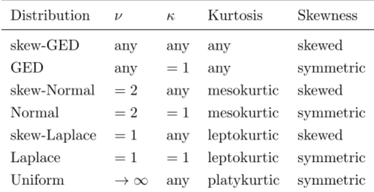
includes several others such as the Gaussian and Laplace - as well as their skewed versions - as special cases; see Table 1 for details. The parameterization of the Skew-GED used here is due Ayebo and Kozubowski (2003).
Ifǫt∼SGED(κ, ν), applying the Jacobian transformation toǫt=yt/σtgives the density ofyt,
1 σt f y t σt = 1 σt ν τΓ(1/ν)
κ
1 +κ2exp
−σ1ν t
κ(y
t−π)+ τ
ν
+
(y
t−π)− τ κ
ν
, yt∈R. (2)
Now, in order to simplify notation, define Yt and Stto be the row vectors of realizations and
volatilities up to time t, i.e. Yt= (Y0, y1, . . . , yt)′ andSt= (σ1, . . . , σt)′. The joint loglikelihood of
(Yn, Sn) of a sample of sizenis
logL(ϕ|Yn, Sn) =
n
X
t=1
−logσt+ log ν τΓ(1/ν)
κ
1 +κ2 −
1
σν t
κ(y
t−π)+ τ
ν
+
(y
t−π)− τ κ
ν
,
(3) whereϕis ap×1 vector of parameters which includesκ,ν and hyperparameters of the volatility. Since performing an inverse probability transformation on a Skew-GED variate is not possible, generating draws from this distribution might seem difficult. However, Ayebo and Kozubowski (2003) exploit the relationship between the Skew-GED and the Gamma distribution to derive a simple pseudorandom number generator algorithm, stated in Algorithm 1 for convenience.
Algorithm 1Skew-GED random number generator.
1: drawG∼Gamma(1/ν,1)
2: drawU ∼Uniform(0,1)
3: if U <1+κ2κ2 then
4: set I=κ1 5: else
6: set I=−κ 7: end if
8: returnX=π+τ IG1/ν ∼SGED(κ, ν)
Table 1. Special cases of the skew-GED distribution.
Distribution ν κ Kurtosis Skewness
skew-GED any any any skewed
GED any = 1 any symmetric
skew-Normal = 2 any mesokurtic skewed
Normal = 2 = 1 mesokurtic symmetric
skew-Laplace = 1 any leptokurtic skewed
Laplace = 1 = 1 leptokurtic symmetric
Uniform → ∞ any platykurtic symmetric
A vast body of research on volatility concerns financial time series, specially daily asset return data. It might be therefore relevant to study their behavior beforehand when considering models for the volatility. Stylized facts found in financial data usually serve as a starting point for proposing model extensions. The pioneer work of Mandelbrot (1963) is perhaps the most important example; he noted that large (small) returns are followed by large (small) returns, giving rise to temporal clusters in their variability. He named this behavior ”volatility clustering”, and it essentially refers to the fact that there is an autoregressive dependence in the volatility, which is a fundamental property of volatility models. Another observation made by the same author is that the distribution of returns are usually leptokurtic, being more propense to outliers than a Gaussian distribution.
Other important stylized facts about financial returns are the leverage effect and long memory in the volatility. The leverage effect was first discovered by Black (1976), which found that volatility responds asymmetrically to negative and positive returns of the same magnitude. This finding is in accordance with the financial theory that a decrease in the price of an asset leads to an increase in its debt/equity ratio (financial leverage) and therefore in its volatility (financial risk), in addition to the increase in the risk that occurs due to the (absolute) variation of returns. The presence of long memory dependence in the volatility was first noted by Ding et al. (1993), which found that the daily absolute returns (a common proxy for the volatility) of the S&P500 presented positive autocorrelations of lag up to and above the order of 2500 and proceeded to propose a model in order to capture this and a myriad other stylized facts.
2.1. Model Evaluation Criteria
likelihood and the number of estimated parameters should be used. The one adopted in this work is the Akaike information criterion (AIC), due Akaike (1974).
The AIC expresses the information lost - measured by the Kullback-Leibler divergence - when approximating the true data generating process by an estimated model. Therefore, minimizing AIC is equivalent to obtaining the best fit. Scaled for sample size, its expression is
AIC(p) =−2n
logL(ϕ|Yn, Sn)−p
,
wherenis the sample size,L(ϕ|Yn, Sn) is the joint likelihood in (3) andpis the number of model
parameters.
Evaluating the goodness of fit of a model is referred to as in-sample evaluation, reflecting the fact that only available information in the moment of estimation is used. However, when there is an interest in predicting future values, out-of-sample evaluation techniques should be used; they are also named ”pseudo-out-of-sample” in order to reflect the fact that some observations are treated as unknown for model estimation but are subsequently used for evaluation.
The out-of-sample comparisons in this work are done in two separate contexts: forecasting volatility and Value-at-Risk. Forecasts in general are obtained as a minimization of a loss func-tion, which penalizes deviations from the true value. A common loss function is the quadratic, expressed asL[σt(h)] =E{[σt(h)−σt+h]2|ψt}whereσt(h) is theh-step ahead forecast. It is a
well-known result [Hamilton (1994)] thatL[σt(h)] is minimal at ˜σt(h) = E(σt+h|ψt), the conditional
expectation ofσt+h over the information setψtand henceforth denoted byσt+h|t.
Forecasts of an estimated model are obtained by straightforward substitution of the popula-tional parameter vectorϕby its estimate ˆϕin the forecast equationσt+h|t; the estimated forecast
is denoted by ˆσt+h|t. The quadratic loss function above can then be used to compare the
over-all forecasting performance across models; its sample counterpart, known as mean squared error (MSE), is expressed by
MSE(k) = 1
k n+k
X
t=n
(ˆσt+h|t−σˇt)2
wherek is the number of performed forecasts, n is the sample size used for estimation and ˇσt is
the true volatility. Usually in practice the true volatility is not available, and must be replaced by a proxy; the absolute demeaned returns is fairly adequate for this purpose, as it has the same unconditional expectation as the volatility.
The Value-at-Risk (VaR) is a very useful tool in risk management. It is defined as the loss corresponding to theα%th percentile of the distribution of returns over the nextN days. In other words, it measures the loss over the nextN days that is exceeded onlyα% of the time. TheN-day
h-step-ahead out-of-sample VaR is expressed as
VaRt+h|t(N, α) =−
√
Nσˆt+h|tSGEDα(κ, ν),
where SGEDα(κ, ν) denotes theα% quantile of the Skew-GED distribution. As stated before, it is
a good idea to calculate this quantile by taking the empirical quantile of a pseudorandom sample
drawn using Algorithm 1. Mathematically, the predicted VaR is essentially theα% quantile of the
distribution of returns, scaled by the forecasted volatility and the square root of the number of days. Since the VaR expresses a positive loss, the negative of this quantile is used.
which is based on Christoffersen (1998). First consider the following indicator function, also known as hit function,
Ht+h|t(N, α) =
(
1, yt+h≤ −VaRt+h|t(N, α)
0, yt+h>−VaRt+h|t(N, α)
defined fort=n, . . . , n+k. If the predicted VaR is correct, it is expected thatP[Ht+h|t(N, α) =
1] =α. Therefore, the quantity
UC(k) =|α−αˆ|,
where ˆα= k1Pn+k
t=nHt+h|t(N, α) is the estimated probability that the loss exceeds the predicted
VaR, can be used to assess peformance between competing models. Although the sign of the difference (α−αˆ) is usually ignored, it has a financial interpretation: if the unconditional coverage is positive (negative), the VaR is said to be conservative (risky), since the loss is being underestimated (overestimated).
In the remainder of this section, we present the three volatility families used in this work.
2.2. Autoregressive Conditional Heteroskedasticity
Introduced in Engle (1982), the Autoregressive Conditional Heteroskedasticity (ARCH) is a model for the square of the volatility, which is a function of past squared returns. The main assumption made in the ARCH family is that by conditioning on the information setψt−1, volatility
at timet is an observable volatility. This essentially means that, once the past of a time series is known, its next-period volatility is deterministic. ARCH-type models are also commonly referred to as conditional volatility models.
The canonical model in the ARCH family is the Generalized ARCH (GARCH) proposed in Bollerslev (1986), which is an extension of the original ARCH model to allow for the squared volatil-ity to also depend on its past values. While the original ARCH model allows for an autoregressive representation in the squared returns, the GARCH allows for an autoregressive moving-average representation.
Two specifications for the volatility in the ARCH family are considered here: the Asymmetric Power ARCH (APARCH) of Ding et al. (1993) and Exponential Generalized ARCH (EGARCH) of Nelson (1991). The APARCH nests at least 9 other popular ARCH models (see Table 2) and the EGARCH is closely related to the Stochastic Volatility model of the next subsection. Since most of the literature on ARCH models consider only one-period (Markovian) dependence on the volatility, that is the case which is presented here.
The APARCH is defined as
yt=σtǫt= (σtδ)1/δǫt, ǫt∼SGED(κ, ν)
σδt =ω+α(|yt−1| −γyt−1)δ+βσδt−1, (4)
fort= 1, . . . , n, whereω >0 is a constant,α≥0 is an autoregressive parameter,−1< γ <1 is a leverage effect parameter,β ≥0 is a moving average parameter andδ≥0 is a power transformation
parameter. These parameter constraints are necessary only to ensure thatσδ
t is positive.
how the parameterγcaptures leverage, letβ = 0 andδ= 2. Then,
σtδ=
(
ω+α(1−γ)2yt−2 1, yt−1≥0,
ω+α(1 +γ)2yt−2 1, yt−1≤0.
Therefore, ifγ >0, negative returns increase the volatility more than positive returns of the same magnitude, which is precisely what the definition of leverage requires.
A last stylized fact captured by the APARCH is long memory in the volatility. Although the precise definition of long memory within volatility models is given in Baillie et al. (1996) as an analogue of Autoregressive Fractionally Integrated Moving Average (ARFIMA) models, Ding et al. (1993) adopt the long memory definition of a slower/hyperbolic decay of autocorrelations,
and show that the APARCH is capable of reproducing that behavior for certain values ofδ. This
parameter allows for greater flexibility within the volatility specification compared to competing ARCH models, since it relaxes the usual assumption that volatility must be expressed either as a conditional standard deviation (δ= 1) or variance (δ= 2).
One-step-ahead predictions under the APARCH model are given by
σδ
t+1|t=ω+α(|yt| −γyt)δ+βσtδ. (5)
The EGARCH is defined as
yt=σtǫt= exp(0.50 logσ2t)ǫt, ǫt∼SGED(κ, ν)
logσt2=ω+θǫt−1+γ(|ǫt−1| −E|ǫt−1|) +βlogσ2t−1, (6)
fort= 1, . . . , n, where ω is a constant,θ is a leverage effect parameter,γ is a magnitude change parameter,βis a moving average parameter andE|ǫt|= 1
Γ(1/ν)
κ
1+κ2
hτΓ(2/α)(1+κ4
)
κ2 +
πΓ(1/α)(1−κ2
)
κ
i
is the expectation of the absolute value ofǫt under the Skew-GED distribution.
The logarithmic transformation in the EGARCH ensures that the volatilityσtis always positive,
and therefore there are no positivity constraints on the parameters. However, in order for the model to properly reproduce the volatility clustering property, it is required that−γ < θ < γandβ≥0. Under these conditions, large (small) innovations will increase (decrease) volatility, as the definition of clustering requires.
Regarding other stylized facts, the EGARCH is capable of capturing the leverage effect through
the parameterθ. If β = 0 and γ = 0, logσ2
t = ω+θǫt−1. That is, for θ < 0, logσt2 is larger
(smaller) than its mean ifǫt−1(and theforeyt−1) is negative (positive). The behavior captured by
the parameterγ is also noteworthy: provided thatγ >0, innovations larger (smaller) than their expectation increase (decrease) volatility.
One-step-ahead forecasts under the EGARCH model are given by
logσ2t+1|t=ω+θǫt+γ(|ǫt| −E|ǫt|) +βlogσt2. (7)
Estimation of ARCH-type models by maximum likelihood is rather straightforward, and pro-ceeds as follows: given a sampleYn= (Y0, y1, . . . , yn)′, set quantities att= 0 at their unconditional
expectations and write the volatility recursively fort = 1, . . . , n using (4) for the APARCH and (6) for the EGARCH. An explicit expression for the joint loglikelihood in (3) as a function of the
Table 2. Special cases of the APARCH model.
Model δ γ(1) β(L) Author
APARCH any any any Ding et al. (1993)
NARCH any = 0 = 0 Higgins and Bera (1992)
AGARCH = 2 any any Meitz and Saikkonen (2011)
GJR-GARCH = 2 any any Glosten et al. (1993)
GARCH = 2 = 0 any Bollerslev (1986)
ARCH = 2 = 0 = 0 Engle (1982)
TGARCH = 1 any any Zakoian (1994)
TARCH = 1 any = 0 Rabemananjara and Zakoian (1993)
Taylor/Schwert = 1 = 0 any Taylor (1986), Schwert (1990)
log-ARCH →0 = 0 = 0 Geweke (1986), Pantula (1986)
algorithm such as the one proposed independently by Broyden (1970), Goldfarb (1970), Fletcher (1970) and Shanno (1970), henceforth denoted as BFGS. For the APARCHϕ= (ω, α, β, γ, δ, κ, ν)′
and for the EGARCHϕ= (ω, θ, γ, β, κ, ν)′.
Due to the practice of setting unobservable quantities att= 0 at their unconditional expecta-tions, some authors refer to the likelihood maximization procedure described above as conditional (or approximate) maximum likelihood estimation. Having such a simple inference procedure is a major comparative advantage of ARCH models, and what makes them so relevant in practice.
2.3. Stochastic Volatility
In the Stochastic Volatility (SV) family, volatility is driven by its own stochastic process. Models in this family have often been used in mathematical Finance to reproduce the behavior of prices in the stock market. Although the model exact origins are somewhat uncertain, the first discrete-time version of the SV was proposed by Taylor (1982). In this canonical version, the log-squared volatility follows a first-order autoregressive process with Gaussian innovations; therefore, it is usually referred to as the lognormal SV model. A slight generalization of this model allowing for returns to be Skew-GED distributed can be defined as
yt=σtǫt= exp(ht/2)ǫt, ǫt∼SGED(κ, ν)
ht+1=µ+φht+σηηt, ηt∼Normal(0,1), (8)
fort= 1, . . . , n, whereht= log(σt2) is the log-squared volatility,ǫtandηtare serially and mutually
independent,µ is a constant, φ is an autoregressive parameter and ση ≥0 is a scale parameter.
The model is initialized withh0= 0, i.e. h1∼Normal(µ, ση2).
As in the EGARCH, the logarithmic transformation ensures that the volatility is always positive
for any parameter values. Furthermore, whenση= 0, the SV model is equivalent to the EGARCH
withφ=β and θ=γ = 0. Since it is essentially an AR(1) model for the log-squared volatility,
properties of the SV are straightforward to derive.
The basic SV model presented in (8) is able to reproduce volatility clustering and leptokurticity, but not long memory or the leverage effect. The leverage effect extension of the lognormal SV was first proposed by Harvey and Shephard (1996), and consists of allowing the previous observation
disturbance ǫt−1 and the current state disturbance ηt to be correlated, by assuming that their
version of the lognormal SV was proposed independently by Harvey (1998) and Breidt et al. (1998), which instead of an AR(1) considered an ARFIMA(1, d, 0) process for the volatility. However, both generalizations require that observations be normally distributed; extending these models for Skew-GED distributed returns is out of the scope of this work and therefore they will not be considered here.
Statistical inference for Stochastic Volatility models is considerably more complex than it is for ARCH models. There have been a myriad techniques proposed to estimate the canon lognormal SV; see the excellent reviews on the subject by Broto and Ruiz (2004) and more recently by Bauwens et al. (2012). The main problem in estimating SV models is that volatility is a function not only of its past but also of the stochastic processηt. Therefore, even after conditioning on past
information, volatility is still an unobservable quantity. In order to illustrate that point further, consider the marginal likelihood ofYn,
L(ϕ|Yn) =f(Yn|ϕ) =
Z
S
f(Yn, Hn|ϕ)dHn=
Z
S
f(Yn|Hn, ϕ)f(Hn|ϕ)dHn, (9)
where Hn = (h1, . . . , hn)′ is the joint vector of log-squared volatilities and S = (0,∞)n is its
corresponding support.
While the expression for f(Yn|Hn, ϕ) is straightforward, the marginal distribution f(Hn|ϕ)
is not available in analytical form. Approximating this distribution - and therefore the joint likelihood - is the main estimation problem in the Stochastic Volatility family. An interesting solution is the importance sampling technique for non-Gaussian and nonlinear state space models proposed independently by Durbin and Koopman (1997) and Shephard and Pitt (1997) and which has been considerably improved upon in the textbook treatment given by Durbin and Koopman (2012). It is sometimes referred to as Monte Carlo Maximum Likelihood Estimation.
Although the ideas of importance sampling are relatively simple, the estimation process is considerably more complex. First, consider the following linear Gaussian model,
xt=ht+ǫt, ǫt∼Normal(0, At),
ht+1=µ+φht+σηηt, ηt∼Normal(0,1), (10)
fort= 1, . . . , n. The model is initialized withh0 = 0, i.e. h1 ∼Normal(µ, σ2η). Denote byg the
densities associated with this linear state space model, and notice that the state equation in (10) is the same as that of the Stochastic Volatility model (8), implying thatf(Hn) =g(Hn).
Now, using the fact that f(Hn,Yn)
g(Hn,Yn) =
f(Yn|Hn)f(Hn)
g(Yn|Hn)g(Hn) =
f(Yn|Hn)
g(Yn|Hn), rewrite the joint likelihood in
(9) as
L(ϕ|Yn) =
Z
S
f(Hn, Yn)dHn=g(Yn)
Z
S
f(Hn, Yn) g(Hn, Yn)
g(Hn|Yn)dHn =Lg(ϕ|Yn)Eg
f(Yn|Hn) g(Yn|Hn)
,
(11) where g(Hn|Yn) is the smoothed Gaussian density, Lg(ϕ|Yn) = g(Yn) is the marginal Gaussian
likelihood andEgdenotes expectation with respect tog(Hn|Yn). The dependence off andgonϕ
was supressed to simplify notation.
Expression (11) was first proposed by Durbin and Koopman (1997) and essentially defines the joint non-Gaussian likelihood (9) as an adjustment to a simple Gaussian density. This adjusment term is readily estimable by importance sampling by takingg(Hn|Yn) as the importance density.
and therefore expression (11) is easily manageable.
In order to completely determineg(Hn|Yn) one must first appropriately specifyxtand Atfor t= 1, . . . , n. Examination of the non-Gaussian likelihood (11) suggests that g(Yn|Hn) should be
as close as possible tof(Yn|Hn) in a neighborhood of their mode. Durbin and Koopman (1997)
suggest using a Laplace approximation of the log-ratio of these densities to determinext,Atand the
mode vector of log-squared volatilitesHn, denoted by ˆHn. Conditional independence of (Hn, Yn)
under both Gaussian and non-Gaussian densities implies that f(Yn|Hn)
g(Yn|Hn) =
Qn
t=1
f(yt|ht)
g(yt|ht); therefore,
the log-ratio between these two densities is given by
l(Hn) = n
X
t=1
[logf(yt|ht)−logg(yt|ht)],
where the dependence ofl on Yn was dropped since it is assumed to be fixed when determining
the mode.
It follows thatxtandAt are obtained as the solutions of∂l(ht)/∂ht= 0 and∂2l(ht)/∂h2t = 0
atht= ˆht, fort= 1, . . . , n. That is,
At=
4
ν2exp νˆht
2
!
κ(yt−π)+ τ
ν
+
(yt−π)− κτ
ν−1
and xt= ˆht−
1 2At+
2
ν. (12)
However, the expressions obtained for xt and At are still functions of the unknown mode ˆht.
Therefore, a Newton-Raphson procedure must be employed to iteratively solve for this mode. Exploiting the linear and Gaussian structure of g(Hn|Yn) allows the use of the Kalman filter
and smoother to calculate the next guess of the iterative procedure; this is computationally more efficient than using the Newton-Raphson algorithm directly. Note that this is only possible due to equality between mean and mode under the Normal distribution.
Denote by at|t−1 = E[ht|Yt−1] and Pt|t−1 = V[ht|Yt−1] the filtered estimate of ht and its
respective variance, by at|t = E[ht|Yt] and Pt|t = V[ht|Yt] the updated estimate of ht and its
respective variance and byat|n =E[ht|Yn] andPt|n =V[ht|Yn] the smoothed estimate of htand
its respective variance. The Kalman filter and smoother for the linear state space model (10) is given in Algorithm 2.
Algorithm 2Kalman filter and smoother for the linear state space model (10).
1: initalizea0|0=µandP0|0= 107 2: fort= 1, . . . , ndo
3: calculate at|t−1=φat−1|t−1+µandPt|t−1=φ2Pt−1|t−1+ση2
4: calculate Ft = Pt|t−1+At, at|t = at|t−1 +Pt|t−1Ft−1(xt−at|t−1) and Pt|t = Pt|t−1 − Pt|t−1Ft−1Pt|t−1
5: end for
6: fort=n−1, . . . ,1 do
7: calculate P∗
t =φPt|tPt+1|t,at|n =at|t+Pt∗(at+1|n−φat|t) andPt|n=Pt|t+Pt|t∗ (Pt+1|n− Pt+1|t)Pt|t∗ .
8: end for
9: returnat|t,Pt|t,at|n,Pt|n,t= 1, . . . , n
To complete the iterative process to obtain the mode, the initialization conditions must be specified. Note that the observation equation in the Stochastic Volatility model (8) implies that
yields the initial values forxtandAt. The entire process of obtaining the mode is summarized in
Algorithm 3.
Algorithm 3Iterative process to approximate the mode off(Hn|Yn).
1: initializeAt= ν42 exp
νlogy2
t
2
hκ(y
t−π)+
τ
ν
+(yt−π)−
κτ
νi−1
andxt= logy2t−12At+ 2
ν
2: compute a first guess ˜ht=at|n,t= 1, . . . , nusing Algorithm 2
3: repeat
4: compute the next guess ˜h+t =at|n,t= 1, . . . , nusing Algorithm 2
5: calculate xtandAtby taking ˜h+t = ˆhtin (12)
6: untilconvergence
7: returnHˆn= (ˆh1, . . . ,ˆhn)′
Convergence to the mode is usually attained with 10 iterations or less. After obtaining the mode, the importance densityg(Hn|Yn) is completely determined and it is possible to draw from
it using the simulation procedure of Shephard (1994b), summarized in Algorithm 4. It should be clear that the mode and random draws obtained from the importance density are conditional on
ϕ= (µ, φ, ση, κ, ν)′ known; the situation whereϕis estimated is considered below.
Algorithm 4Simulation procedure for drawing fromg(Hn|Yn).
1: computeat|t, at|t−1, Ptt|t−1 andPt|t,t= 1, . . . , nusing steps 1-5 of Algorithm 2.
2: drawhn|Yn∼Normal(an|n, Pn|n).
3: fort=n−1, . . . ,1 do
4: drawht|ht+1∼Normal
at|t+
φPt|t(ht+1−at+1|t)
Pt+1|t , Pt|t−
φ2P2
t|t
Pt+1|t
5: end for
6: returnHn= (h1, . . . , hn)′
When simulating fromg(Hn|Yn), computational efficiency can be increased by employing
an-tithetic variables. As Durbin and Koopman (2012) defines, an anan-tithetic variable is a function
of a random drawn of Hn which is equiprobable with Hn and which increases the efficiency of
the estimation when included in the drawing process. The first antithetic variable used here is ˇ
Hn= 2 ˆHn−Hn; sinceHn is Gaussian with mean ˆHn, it is straightforward to verify that ˇHn has
the same distribution asHn. Whenever this antithetic variable is used, the simulation sample is
said to be balanced for location.
The second antithetic variable used here was developed by Durbin and Koopman (1997). Let
Un be the vector of thenNormal(0,1) variables used in the simulation procedure to generateHn
and letc =U′
nUn; then c ∼ χ2n, where χ2n denotes a chi-squared distribution with n degrees of
freedom. For a given value ofc letq =P(χn2 < c) =F(c) be the distribution function of c and
´
c=F−1(1−q) be the quantile function ofc; moreover, note thatcand ´chave the same distribution.
Noting thatcand (Hn−Hˆn)/√care independently distributed, two additional antithetic variables
can be constructed: ´Hn = ˆHn+
q
´
c
c(Hn−Hˆn) and `Hn = ˆHn+
q
´
c
c( ˇHn−Hˆn). When these two
antithetics are used, the simulation sample is said to be balanced for scale. By using both types
of antithetic variables a set of four equiprobable values of Hn are obtained for each run of the
simulation procedure, yielding a simulation sample which is balanced for both location and scale. The primary objective of importance sampling here is to estimate the unknown parameter vectorϕ. In order to accomplish that, it is first necessary to estimate the joint likelihood (11) by
is
log ˆL(ϕ|Yn) = logLg(ϕ|Yn) + log ¯w+ S
2
w
2Nw¯2, (13)
whereNis the number of simulations and ¯w= (1/N)PN
i=1wi, withwi=w(Hn(i), Yn) =f(Hn(i), Yn)/g(Hn(i), Yn)
denoting the importance weights andHn(i) = (h(1i), . . . , h (i)
n )′ denoting the vector of log-squared
volatilities generated for i = 1, . . . , N. The last term is a necessary bias correction when tak-ing the logarithm of the likelihood, since E[log ¯w] 6= logEg[wi] and its numerator is given by
S2
w=N1−1
PN
i=1(wi−w¯)2; see Durbin and Koopman (1997) for a detailed proof.
The Gaussian loglikelihood logLg(ϕ|Yn) can be evaluated by the Kalman filter using the
predic-itve error decomposition. That is, after obtaining at|t and Ft from steps 1-5 of Algorithm 2,
compute
logLg(ϕ|Yn) =−1
2
n
X
t=1
log 2π+ logFt+
(xt−at)2 Ft
. (14)
The only quantity remaining to be determined for the estimation process are the impor-tance weights wi. Since f(yt|h(ti)) is given in (2) by taking σt = exp(h(ti)/2) and g(yt|h(ti)) =
Normal(h(ti), At),
wi= exp
(
−12
n
X
t=1
"
h(ti)+
2 exp(νh(ti)/2)
κ(y
t−π)+ τ
ν
+
(y
t−π)− κτ
ν
−2 log
ν
τΓ(1/ν)
κ
1 +κ2
−log 2π−logAt−
xt−h(ti)
√ At
!2#)
. (15)
After drawing N samples of Hn and calculating the loglikelihood estimate (13) it is possible
to maximize it with respect to ϕ using an iterative maximization process such as the BFGS.
Each iteration of the procedure is started with an initial guess ofϕgiven by first maximizing the approximate joint loglikelihood
log ˆL(ϕ|Yn)≈logLg(ϕ|Yn) + logw( ˆHn), (16)
wherew( ˆHn) =f( ˆHn, Yn)/g( ˆHn, Yn).
The entire estimation procedure of the Stochastic Volatility model (8) using importance sam-pling can be summarized in Algorithm 5
Algorithm 5Importance sampling estimation ofϕ.
1: initialize with a guess ˜ϕ 2: repeat
3: compute ˆHn = (ˆh1, . . . ,ˆhn)′ using Algorithm 3 conditional on ˜ϕ.
4: compute an intermediate guess ˇϕby maximizing the approximate loglikelihood (16) using
the BFGS numerical procedure conditional on ˜ϕ
5: sampleHn(i),i= 1, . . . , N using Algorithm 4 and calculate the antithetic variables ˇHn, ´Hn
and `Hn conditional on ˇϕ
6: evaluate the Gaussian loglikelihood in (13) using steps 1-5 of Algorithm 2 conditional on ˇϕ
7: compute importance weights wi, i= 1, . . . , N using (15) conditional on ˇϕ
8: estimate the joint loglikelihood (13) and compute a new guess ˜ϕusing the BFGS algorithm
conditional on ˇϕ
9: untilconvergence to ˆϕ= arg max
ϕ∈Φ
L(ϕ|Yn)
For numerical stability of the optimization process, Durbin and Koopman (2012) suggest using the same random numbers to generate the states from the importance density in step 5 of Algorithm 5 for each value ofϕ. This will ensure that the loglikelihood is a smooth function of the parameters. Two other functions of interest to estimate using importance sampling are the smoothed states
at|n = E(ht|Yn) and their respective variances Pt|n = V(ht|Yn), for t = 1, . . . , n. A simple
manipulation of conditional densities similar to that done in (11) yields their respective expressions,
at|n=
Eg[htw(ht, Yn)]
Eg[w(ht, Yn)] and Pt|n = Eg[h2
tw(ht, Yn)]
Eg[w(ht, Yn)] −a
2
t|n. (17)
Conditional on ˆϕ, their respective estimates are given by
ˆ
at|n= N
X
i=1
˜
w(ti)h
(i)
t and Pˆt|n=
N
X
i=1
˜
w(ti)h
(i)2
t −aˆ2t|n, (18)
fort= 1, . . . , n, where ˜w(ti)=w(h
(i)
t , Yn)/PNi=1w(H (i)
n , Yn) are the normalized importance weights.
One-step-ahead forecasts under the SV model are given by
ht+1|t=µ+φht. (19)
2.4. Non-Gaussian State Space Models
The last and most recent family of models considered here is the Non-Gaussian State Space Models (NGSSM) family proposed in Gamerman et al. (2013) and extended in Pinho et al. (2016) to include heavy-tailed distributions. In the volatility context, the NGSSM is essentially a dynamic scale model with Beta innovations, allowing for a variety of distributions for the observations, including most members of the exponential family. It is defined as
yt=σtǫt=λt−1/νǫt, ǫt∼SGED(κ, ν)
λt+1 =w−t+11λtςt+1, ςt+1|Yt∼Beta (wat,(1−wt+1)at), (20)
for t = 1, . . . , n, where λt = σ−νt > 0 is the dynamic level, 0 < w ≤ 1 is an autoregressive
parameter, at is defined in (22) and wt = exp{Ψ(wat−1)−Ψ(at−1)} with Ψ(·) denoting the
digamma function. The model is initialized with λ0|Y0 ∼ Gamma(a0, b0) where a0 and b0 are
positive arbitrary constants.
Since the Non-Gaussian State Space Models are relatively recent in the literature, the only known extension proposed so far in this family is the heavy-tailed distribution and scale modelling generalization proposed by Pinho et al. (2016). Therefore, although it has a very flexible form, in terms of stylized facts the basic NGSSM model (20) can only reproduce volatility clustering and leptokurticity.
The role of the parameter w is similar to that of a discount factor: only 100wt% of the
in-formation (in terms of precision) is retained from one period to another. To see this, note that
V(λt|Yt−1) =wt−1V(λt−1|Yt−1). Note also thatE(λt|Yt−1) =E(λt−1|Yt−1); that is, the conditional
mean of the dynamic level does not change over time.
the logarithm on both sides of the evolution equation in (20), it becomes
log(λt) = log(λt−1) +ςt∗,
whereς∗
t = log(ςt/wt)∈R. This equation is very similar to that of a local level model, therefore
reinforcing the idea that the NGSSM has by definition a nonstationary variance (though it has a stationary mean).
Analogous to the SV model, in the NGSSM volatility is also driven by its own stochastic process. However, in terms of inference the latter has several advantages over the former. Part 3 of Theorem 1 in Gamerman et al. (2013) states that under the NGSSM it is possible to analytically integrate out the volatilities in (9), thus allowing for exact likelihood inference. This procedure yields a marginal loglikelihood which depends only onϕandYn, given by
logL(ϕ|Yn) =
n
X
t=1
(
log Γ(1/ν+at|t−1) + log
ν τΓ(1/ν)
κ
1 +κ2
+at|t−1logbt|t−1−log Γ(at|t−1)
−(1/ν+at|t−1) log
κ(yt−π)+ τ
ν
+
(yt−π)− κτ
ν+bt|t−1
)
, (21)
where
at|t−1=wat−1, bt|t−1=wtbt−1, (22)
at=at|t−1+ 1/ν, bt=bt|t−1+
κ(y
t−π)+ τ
ν
+
(y
t−π)− κτ
ν
.
Estimation of ϕ= (w, κ, ν)′ proceeds by straightforward maximization of the loglikelihood in
(21) using the BFGS algorithm. After estimatingϕ, it is possible to use the results from Theorem 2 and Parts 1 and 2 of Theorem 1 in Gamerman et al. (2013) to obtain exact filtered and smoothed estimates of the joint vectorLn = (λ1, . . . , λn)′. The filtering procedure is given in Algorithm 6
and the smoothing procedure is given in Algorithm 7.
Algorithm 6Non-Gaussian State Space Model filter.
1: initalizea0= 100 andb0= 100 2: fort= 1, . . . , ndo
3: calculate at|t−1=wat−1 andbt|t−1=wtbt−1
4: calculate at=at|t−1+ 1/ν andbt=bt|t−1+
hκ(y
t−π)
+
τ
ν
+(yt−π)−
κτ
νi
5: drawλt|Yt, ϕ∼Gamma(at, bt)
6: end for
7: returnLn= (λ1, . . . , λn)′
Algorithm 7Non-Gaussian State Space Model smoother.
1: computeλt,atandbt,t= 1, . . . , n using Algoritm
2: drawλn|Yn, ϕ∼Gamma(an, bn)
3: fort=n−1, . . . ,1 do
4: drawλt|t+1=λt−wtλt+1|λt+1, Yt, ϕ∼Gamma((1−wt)at, bt).
5: calculateλt=λt|t+1+wtλt+1 6: end for
The one-step-ahead predictive distribution of the dynamic level is given by
λt+1|Yt, ϕ∼Gamma(at+1|t, bt+1|t), (23)
whereat+1|t=wtat andbt+1|t=wtbt. Forecasts are calculated by taking a summary measure of
this distribution; its expectation is given by
ˆ
λt+1|t= at+1|t bt+1|t
. (24)
3. APPLICATION
In this section an application concerning a sample of 4 daily asset return series, from Jan-2000 to Jan-2016 is made to illustrate the volatility models and evaluation criteria presented so far. The assets are:
1. Ibovespa (BOVESPA): an index composed by a theoretical portfolio with the stocks that accounted for 80% of the volume traded in the last 12 months and that were traded at least on 80% of the trading days in the BM&F Bovespa Stock Exchange. In average the components of Ibovespa represent 70% of all the stock value traded.
2. Hang Seng Index (HANGSENG): a freefloat-adjusted market capitalization-weighted stock market index in Hong Kong. It is used to record and monitor daily changes of the largest companies on the Hong Kong stock market and is the main indicator of the overall mar-ket performance in Hong Kong. Its 50 constituent companies represent about 58% of the capitalisation of the Hong Kong Stock Exchange.
3. Merval Index (MERVAL): a price-weighted index, calculated as the market value of a portfolio of stocks selected using the 80% volume and 80% trading days criteria in the last semester in the Buenos Aires Stock Exchange.
4. S&P/TSX Composite Index (SPTSX): an index of the stock (equity) prices of the largest companies on the Toronto Stock Exchange as measured by market capitalization. The listed companies in this index account for about 70% of market capitalization for all Canadian-based companies listed.
Taking pt to represent the price of the asset (index value) at time t, daily return series are
calculated asyt= 100×[log(pt)−log(pt−1)] minus its mean. Of the 4000 collected observations, k= 1000 - or about 4 years, from 2012 to 2016 - are reserved for forecasting evaluation, while the
remainingn = 3000 - or about the remaining 12 years, from 2000 to 2012 - are used for model
estimation and loglikelihood evaluation.
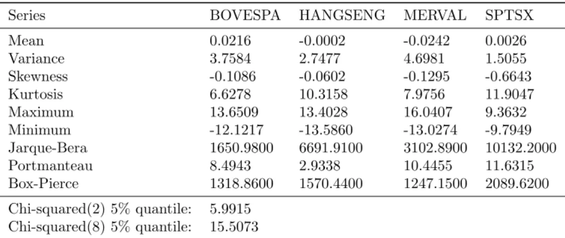
Table 3 presents summary statistics and autocorrelation tests for the return data. Some obser-vations are in order:
· The ”Portmanteau” statistic reported on the table refers to the nonparametric test proposed
in Francq and Zakoian (2000) to test for joint absence of autocorrelation. The test is robust to higher moment dependency in the data, such as conditional heteroskedasticity. The null hypothesis is that the autocorrelations from orders 1 throughmare jointly equal zero. Here
Table 3. Summary statistics for the logreturns series.
Series BOVESPA HANGSENG MERVAL SPTSX
Mean 0.0216 -0.0002 -0.0242 0.0026
Variance 3.7584 2.7477 4.6981 1.5055
Skewness -0.1086 -0.0602 -0.1295 -0.6643
Kurtosis 6.6278 10.3158 7.9756 11.9047
Maximum 13.6509 13.4028 16.0407 9.3632
Minimum -12.1217 -13.5860 -13.0274 -9.7949
Jarque-Bera 1650.9800 6691.9100 3102.8900 10132.2000
Portmanteau 8.4943 2.9338 10.4455 11.6315
Box-Pierce 1318.8600 1570.4400 1247.1500 2089.6200
Chi-squared(2) 5% quantile: 5.9915
Chi-squared(8) 5% quantile: 15.5073
· The ”Box-Pierce” statistic refers to the conventional Box-Pierce test, but applied to the
square of the series. As proved in Francq and Zakoian (2010), it is equivalent to the LM statistic to test for conditional heteroskedasticity. The null hypothesis is that the
autocor-relations of the squares from orders 1 throughm are jointly equal zero. As in the previous
test,m≈log(n) = 8.
· Results from the first portmanteau test indicate that at the 5% level there is no information in the conditional mean, whereas the second portmanteau test indicate that there is in fact temporal information in the conditional variance, for all series. This is ideal for an application of volatility models, since it is only necessary to model the conditional variance.
· The Jarque-Bera statistic follows a Chi-Squared(2) distribution, of which the 5% quantile
is also present in the table. The null hypothesis for this is test is that data comes from a Normal distribution, and it essentially compares deviations of skewness and kurtosis from the Gaussian (which are respectively 0 and 3) with that of the data. The hypothesis of gaussianity is rejected for all 4 series.
· In addition to non-gaussianity, the presence of significant negative skewness and excess kur-tosis exhibited in these data are also stylized facts of financial series, as discussed in section 2 of this work.
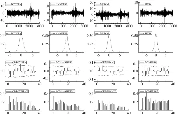
In accordance to these points, Figure 1 illustrates the time series, standardized density,
auto-correlation function1 (ACF) and ACF of squares for all 4 asset returns. The ACF plots include a
nonparametric significance band, used in the portmanteau test and the ACF squared plots include the standard Bartlett significance bands, used in the Box-Pierce test.
Parameter estimates and respective confidence intervals for all 4 volatility models presented
are contained in Table 4, and their respective CPU time spent2 are presented in Table 5. Some
interesting points to note are:
· In the APARCH, EGARCH and NGSSM models, the asymmetry parameter κ is always
greater than 1 and the tail thickness parameter ν is always between 1 and 2. The
corre-sponding distribution in this case is skewed to the right and is between a skew-Laplace and a skew-Normal in terms of tail thickness.
1The maximum lag chosen to display the ACF ism≈min(10×log 10(n), n−1) = 35.
Table 4. Estimated parameters and confidence intervals (in brackets) for the logreturn data.
Series BOVESPA HANGSENG MERVAL SPTSX
APARCH
ω 0.058622 0.018694 0.13529 0.01639
[0.0342;0.1006] [0.012;0.0291] [0.0705;0.2595] [0.0113;0.0237]
α 0.062633 0.065541 0.088835 0.051107
[0.0432;0.0907] [0.0511;0.0841] [0.0619;0.1275] [0.0318;0.0822]
β 0.91762 0.93508 0.86968 0.93338
[0.893;0.9429] [0.9203;0.9501] [0.8335;0.9075] [0.9152;0.9519]
γ 0.58883 0.50395 0.19022 0.8101
[0.2832;0.7859] [0.2984;0.6648] [0.0798;0.2961] [-0.1653;0.9844]
δ 1.3852 1.17 2.2051 1.3754
[0.9518;2.0161] [0.8287;1.6518] [1.5833;3.0711] [1.0295;1.8377]
κ 1.0559 1.0465 1.0556 1.1154
[1.0165;1.0968] [1.0093;1.0851] [1.0143;1.0986] [1.0756;1.1567]
ν 1.7018 1.4687 1.2887 1.5771
[1.581;1.8319] [1.359;1.5873] [1.2047;1.3786] [1.4663;1.6962]
EGARCH
ω 0.091424 0.055073 0.079945 0.047208
[0.0635;0.1193] [0.0389;0.0713] [0.052;0.1079] [0.032;0.0624]
β 0.97593 0.98731 0.9719 0.98538
[0.9612;0.9851] [0.9803;0.9918] [0.9549;0.9826] [0.9785;0.9901]
θ -0.077507 -0.06125 -0.051785 -0.080142
[-0.1007;-0.0543] [-0.0813;-0.0412] [-0.0747;-0.0288] [-0.1016;-0.0587]
γ 0.12986 0.12707 0.19286 0.11266
[0.0947;0.1651] [0.0985;0.1556] [0.1479;0.2379] [0.0822;0.1431]
κ 1.0556 1.0467 1.0535 1.1128
[1.0162;1.0965] [1.01;1.0848] [1.0184;1.0898] [1.073;1.1541]
ν 1.6912 1.4615 1.2631 1.5637
[1.5716;1.82] [1.3527;1.5789] [1.1823;1.3495] [1.4536;1.6821]
NGSSM
w 0.94114 0.95087 0.92875 0.94284
[0.928;0.952] [0.9394;0.9603] [0.9138;0.9413] [0.9294;0.9539]
κ 1.0316 1.0404 1.0429 1.115
[0.9927;1.072] [1.0055;1.0766] [1.0026;1.0848] [1.0767;1.1546]
ν 1.8205 1.4842 1.4745 1.7125
[1.6724;1.9816] [1.3702;1.6077] [1.3596;1.5992] [1.5747;1.8625]
SV
µ 0.019837 0.0040052 0.038969 -0.0024313
[0.0078;0.0318] [-0.0009;0.0089] [0.0203;0.0576] [-0.0075;0.0026]
φ 0.98102 0.99159 0.96472 0.98868
[0.9705;0.9916] [0.9861;0.9971] [0.9492;0.9803] [0.9818;0.9956]
ση 0.1263 0.11061 0.23097 0.13582
BOVESPA
0 1000 2000 3000
-10 0
10 BOVESPA HANGSENG
0 1000 2000 3000
-10 0
10 HANGSENG MERVAL
0 1000 2000 3000
-10 0 10
20 MERVAL SPTSX
0 1000 2000 3000
0 10 SPTSX
BOVESPA
-5 0 5
0.2
0.4 BOVESPA HANGSENG
-5 0 5
0.25
0.50 HANGSENG MERVAL
-5 0 5
0.25
0.50 MERVAL SPTSX
-5 0 5
0.25 0.50 SPTSX
ACF-BOVESPA
0 20 40
0.0
ACF-BOVESPA ACF-HANGSENG
0 20 40
-0.1 0.0
0.1 ACF-HANGSENG ACF-MERVAL
0 20 40
-0.1 0.0
0.1 ACF-MERVAL ACF-SPTSX
0 20 40
-0.1 0.0
0.1 ACF-SPTSX
ACF-BOVESPA^2
0 20 40
0.2
0.4 ACF-BOVESPA^2 ACF-HANGSENG^2
0 20 40
0.2
0.4 ACF-HANGSENG^2 ACF-MERVAL^2
0 20 40
0.2
0.4 ACF-MERVAL^2 ACF-SPTSX^2
0 20 40
0.2
0.4 ACF-SPTSX^2
Figure 1. Time series, standardized densities, ACF and ACF-squared of logreturn data.
Table 5. CPU time spent (in seconds) in the estimation of each model.
Series BOVESPA HANGSENG MERVAL SPTSX
APARCH 3.094 2.797 3.235 3.453
EGARCH 1.829 1.703 1.687 1.438
NGSSM 0.859 0.828 0.86 0.953
· In the SV model the hypotheses κ = 1 and ν = 2 could not be rejected at the 5% level, for all 4 series. Although the lack of skewness in the unconditional distribution of returns is somewhat surprising, unconditional mesokurtosis is actually expected in a SV model. As discussed earlier, the work of Carnero et al. (2004) argues that in comparison to ARCH-type models the lognormal SV can reproduce a much wider range of behavior (especially excess unconditional leptokurtosis) without the inclusion of additional parameters. Since when
κ= 1 andν = 2 the skew-GED distribution reduces to the Gaussian, the re-estimated SV
model under these assumptions actually corresponds to the lognormal SV. Computational efficiency gains to relaxing the skew-GED assumption are substantial, reducing CPU time by a factor greater than 5.
· There is a vast difference between computational time amongst models: estimating the
NGSSM takes the least amount of time, and it is followed in this sense by the EGARCH, the APARCH and the SV. Although the absolute difference in seconds might not appear large, the relative difference is striking. For example, for the BOVESPA series, the SV model takes roughly 83 times as long as the NGSSM model, the APARCH takes about 4 times and the EGARCH about 2 times. Relative computational efficiency is especially important when the number of series considered increases exponentially, as is the case in a large portfolio management.
· All models display a strong persistence in the volatility; this is measured in the APARCH
byα+β, in the EGARCH byβ, in the NGSSM by wand in the SV by φ. This is also a
stylized fact of financial series and it is to be expected. However, it is worth noticing that the hypothesis of stationarity (tested by veryfing that the value 1 is contained in the confidence intervals for these parameters) can not be rejected at 5% for any of these models - except the NGSSM, which is nonstationary by construction - for any of the series.
· The leverage effect is significant in the EGARCH for all 4 series, and in APARCH for all
but the SPTSX. The estimated coefficients also have the expected sign: positive γ in the
APARCH and negativeθin the EGARCH.
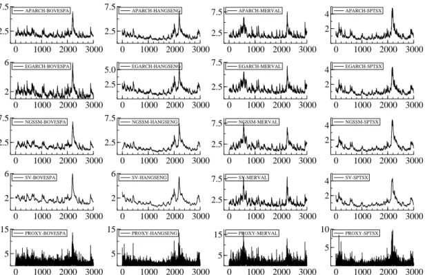
After estimating model parameters, smoothed volatility estimates can also be obtained for each model. They are contained in Figure 2 for each model and series, along with the corresponding proxy for the true volatility (absolute value of logreturns). Another quantity of interest is the one-step-ahead forecast of the volatility, which is calculated recursively for thek= 1000 reserved observations for all models and series, and shown in Figure 3 along with the absolute returns for
these observations. When calculating the forecasts, it is assumed that the sample sizen = 3000
used for estimation is enough to ensure that estimated parameters remain relatively constant over time, so that the models do not need to be reestimated after each new observation is included in the sample. The smoothed and one-step-ahead volatility forecasts seem to closely reproduce the observed behavior patterns in the data.
Although the above information is useful to illustrate and understand the behavior of volatility and financial series in general, it contributes little to the issue of model comparison. The adequate statistical tools for that end are the evaluation criteria introduced in section 2.1. Table 6 contains the computed criteria for all estimated models so far.
APARCH-BOVESPA
0 1000 2000 3000
2.5
7.5 APARCH-BOVESPA APARCH-HANGSENG
0 1000 2000 3000
2.5
7.5 APARCH-HANGSENG APARCH-MERVAL
0 1000 2000 3000
2.5
7.5 APARCH-MERVAL APARCH-SPTSX
0 1000 2000 3000
2
4 APARCH-SPTSX
EGARCH-BOVESPA
0 1000 2000 3000
2
6 EGARCH-BOVESPA EGARCH-HANGSENG
0 1000 2000 3000
2.5
5.0 EGARCH-HANGSENG EGARCH-MERVAL
0 1000 2000 3000
2.5
7.5 EGARCH-MERVAL EGARCH-SPTSX
0 1000 2000 3000
2
4 EGARCH-SPTSX
NGSSM-BOVESPA
0 1000 2000 3000
2.5
7.5 NGSSM-BOVESPA NGSSM-HANGSENG
0 1000 2000 3000
2.5
7.5 NGSSM-HANGSENG NGSSM-MERVAL
0 1000 2000 3000
2.5
7.5 NGSSM-MERVAL NGSSM-SPTSX
0 1000 2000 3000
2
4 NGSSM-SPTSX
SV-BOVESPA
0 1000 2000 3000
2
6 SV-BOVESPA SV-HANGSENG
0 1000 2000 3000
2
6 SV-HANGSENG SV-MERVAL
0 1000 2000 3000
2.5
7.5 SV-MERVAL SV-SPTSX
0 1000 2000 3000
2
4 SV-SPTSX
PROXY-BOVESPA
0 1000 2000 3000
5
15 PROXY-BOVESPA PROXY-HANGSENG
0 1000 2000 3000
5
15 PROXY-HANGSENG PROXY-MERVAL
0 1000 2000 3000
5
15 PROXY-MERVAL PROXY-SPTSX
0 1000 2000 3000
5
10 PROXY-SPTSX
Figure 2. Smoothed volatility estimates and absolute returns.
APARCH-BOVESPA
0 500 1000
1.5
2.5 APARCH-BOVESPA APARCH-HANGSENG
0 500 1000
1
2 APARCH-HANGSENG APARCH-MERVAL
0 500 1000
3
5 APARCH-MERVAL APARCH-SPTSX
0 500 1000
0.5
1.5 APARCH-SPTSX
EGARCH-BOVESPA
0 500 1000
1
3 EGARCH-BOVESPA EGARCH-HANGSENG
0 500 1000
1
2 EGARCH-HANGSENG EGARCH-MERVAL
0 500 1000
2
4 EGARCH-MERVAL EGARCH-SPTSX
0 500 1000
0.5
1.5 EGARCH-SPTSX
NGSSM-BOVESPA
0 500 1000
1
3 NGSSM-BOVESPA NGSSM-HANGSENG
0 500 1000
1
2 NGSSM-HANGSENG NGSSM-MERVAL
0 500 1000
2
4 NGSSM-MERVAL NGSSM-SPTSX
0 500 1000
0.5
1.5 NGSSM-SPTSX
SV-BOVESPA
0 500 1000
1.5
2.5 SV-BOVESPA SV-HANGSENG
0 500 1000
1
2 SV-HANGSENG SV-MERVAL
0 500 1000
1 3
SV-MERVAL SV-SPTSX
0 500 1000
0.5
1.5 SV-SPTSX
PROXY-BOVESPA
0 500 1000
2
4 PROXY-BOVESPA PROXY-HANGSENG
0 500 1000
2.5
5.0 PROXY-HANGSENG PROXY-MERVAL
0 500 1000
5
10 PROXY-MERVAL PROXY-SPTSX
0 500 1000
1
3 PROXY-SPTSX