FUNDAÇÃO GETÚLIO VARGAS ESCOLA DE ECONOMIA DE SÃO PAULO
EDUARDO MORATO MELLO
IN SEARCH OF EXCHANGE RATE PREDICTABILITY
A Study about Accuracy, Consistency, and Granger Causality of Forecasts Generated by a Taylor Rule Model
EDUARDO MORATO MELLO
IN SEARCH OF EXCHANGE RATE PREDICTABILITY
A Study about Accuracy, Consistency, and Granger Causality of Forecasts Generated by a Taylor Rule Model
Dissertação apresentada à Escola de Economia de São Paulo da Fundação Getúlio Vargas, como requisito para a obtenção de título de Mestre em Finanças e Economia.
Campo do conhecimento: Finanças Internacionais
ORIENTADOR: Prof. Dr. Paulo Sérgio Tenani
Mello, Eduardo Morato.
In Search of Exchange Rate Predictability - A Study about Accuracy, Consistency, and Granger Causality of Forecasts Generated by a Taylor Rule Model / Eduardo Morato Mello. - 2015.
81 f.
Orientador: Paulo Sérgio Tenani
Dissertação (MPFE) - Escola de Economia de São Paulo. 1. Taxas de juros. 2. Regra de Taylor. 3. Taxas de câmbio. 4. Câmbio - Previsões. I. Tenani, Paulo Sérgio. II. Dissertação (MPFE) - Escola de Economia de São Paulo. III. Título.
EDUARDO MORATO MELLO
IN SEARCH OF EXCHANGE RATE PREDICTABILITY
A Study about Accuracy, Consistency, and Granger Causality of Forecasts Generated by a Taylor Rule Model
Dissertação apresentada à Escola de Economia de São Paulo da Fundação Getúlio Vargas, como requisito para a obtenção de título de Mestre em Finanças e Economia.
Campo do conhecimento: Finanças Internacionais
Data de Aprovação: ___/___/___
Banca examinadora:
______________________________________ Prof. Dr. Paulo Sérgio Tenani (Orientador) FGV-EAESP
______________________________________ Prof. Dr. Emerson Fernandes Marçal
FGV- EESP
______________________________________ Prof. Dr. Leonel Molero Pereira
AGRADECIMENTOS
Expresso meus sinceros agradecimentos a todos que contribuíram para a realização da presente obra:
Ao Prof. Paulo Sérgio Tenani, pela orientação e incentivo durante o desenvolvimento deste trabalho;
Ao Prof. Emerson Fernandes Marçal, pela troca de ideias e sugestões; Ao Prof. Leonel Molero Pereira, pelas críticas construtivas;
À toda equipe do Banco Natixis pelo apoio, em especial ao João Luiz Macedo;
À todos os colegas, professores e monitores do Mestrado Profissional em Finanças e Economia, MPFE, pelo aprendizado;
Aos colegas, e agora amigos, Mateus Vidigal e David Vicentin, pela troca de ideias e sugestões;
Aos estimados colegas do MPFE André da Cunha Scalco, Eric William Picin e Rafael Keiti Oiski Grunho de Souza pela ajuda na implementação do procedimento bootstrap num
RESUMO
Este estudo investiga o poder preditivo fora da amostra, um mês à frente, de um modelo baseado na regra de Taylor para previsão de taxas de câmbio. Revisamos trabalhos relevantes que concluem que modelos macroeconômicos podem explicar a taxa de câmbio de curto prazo. Também apresentamos estudos que são céticos em relação à capacidade de variáveis macroeconômicas preverem as variações cambiais. Para contribuir com o tema, este trabalho apresenta sua própria evidência através da implementação do modelo que demonstrou o melhor resultado preditivo descrito por Molodtsova e Papell (2009), o “symmetric Taylor rule model with heterogeneous coefficients, smoothing, and a constant”. Para isso, utilizamos uma
amostra de 14 moedas em relação ao dólar norte-americano que permitiu a geração de previsões mensais fora da amostra de janeiro de 2000 até março de 2014. Assim como o critério adotado por Galimberti e Moura (2012), focamos em países que adotaram o regime de câmbio flutuante e metas de inflação, porém escolhemos moedas de países desenvolvidos e em desenvolvimento. Os resultados da nossa pesquisa corroboram o estudo de Rogoff e Stavrakeva (2008), ao constatar que a conclusão da previsibilidade da taxa de câmbio depende do teste estatístico adotado, sendo necessária a adoção de testes robustos e rigorosos para adequada avaliação do modelo. Após constatar não ser possível afirmar que o modelo implementado provém previsões mais precisas do que as de um passeio aleatório, avaliamos
se, pelo menos, o modelo é capaz de gerar previsões “racionais”, ou “consistentes”. Para isso,
usamos o arcabouço teórico e instrumental definido e implementado por Cheung e Chinn (1998) e concluímos que as previsões oriundas do modelo de regra de Taylor são
“inconsistentes”. Finalmente, realizamos testes de causalidade de Granger com o intuito de
verificar se os valores defasados dos retornos previstos pelo modelo estrutural explicam os valores contemporâneos observados. Apuramos que o modelo fundamental é incapaz de antecipar os retornos realizados.
ABSTRACT
This study investigates whether a Taylor rule-based model provides short-term, one-month-ahead, out-of-sample exchange-rate predictability. We review important research that concludes that macroeconomic models are able to forecast exchange rates over short horizons. We also present studies that are skeptical about the forecast predictability of exchange rates with fundamental models. In order to provide our own evidence and contribution to the discussion, we implement the model that presents the strongest results in Molodtsova and
Papell’s (2009) influential paper, the “symmetric Taylor rule model with heterogeneous coefficients, smoothing, and a constant.” We use a sample of 14 currencies vis-à-vis the US dollar to make out-of-sample monthly forecasts from January 2000 to March 2014. As with the work of Galimberti and Moura (2012), we focus on free-floating exchange rate and inflation-targeting economies, but we use a sample of both developed and developing countries. In line with Rogoff and Stavrakeva (2008), we find that the conclusion about a
model’s out-of-sample exchange-rate forecast capability largely depends on the test statistics used: it is necessary to use stringent and robust test statistics to properly evaluate the model. After concluding that it is not possible to claim that the forecasts of the implemented model are more accurate than those of a random walk, we inquire as to whether the fundamental model is at least capable of providing “rational,”or “consistent,” predictions. To test this, we adopt the theoretical and procedural framework laid out by Cheung and Chinn (1998). We find that the implemented Taylor rule model’s forecasts do not meet the “consistent” criteria.
Finally, we implement Granger causality tests to verify whether lagged predicted returns are able to partially explain, or anticipate, the actual returns. Once again, the performance of the structural model disappoints, and we are unable to confirm that the lagged forecasted returns antedate the actual returns.
LISTA DE ILUSTRAÇÕES
Chart 1 Economic predictors of exchange rates ... 17
Chart 2 – Molodtsova and Papell (2009) model taxonomy ... 25
Chart 3 – Consistency criteria – requirements for the forecast and actual series ... 30
Chart 4 – A procedure to test for unit roots ... 32
Chart 5 – Graphical example of two cointegrated series ... 33
Chart 6 – Variables transformation ... 43
Chart 7 – Roadmap to the implemented tests ... 44
Chart 8 Random walk behavior of an asset as discount rates near unity ... 61
Chart 9 Bootstrap algorithm for estimating standard errors ... 64
LISTA DE TABELAS
Table 1 – Diebold-Mariano and Clark-West asymptotic tests results ... 46
Table 2 – Squared forecast error differences ... 48
Table 3 – Unit root test results ... 50
Table 4 – Cointegration test results ... 52
Table 5 – Unitary elasticity test results ... 53
Table 6 – Granger causality test results log-returns of exchange rates ... 54
LISTA DE ABREVIATURAS
ADF: Augmented Dickey-Fuller, refers to a unit root test CIRP: Covered interest rate parity
CPI: Consumer price index
CW: Clark-West, a comparison test for predictive accuracy DM: Diebold-Mariano, a comparison test for predictive accuracy GDP: Gross domestic product
HP: Hodrick-Prescott, refers to the HP-filter to estimate the potential output IFS: International Financial Statistics
IMF: International Monetary Fund
IPSA: Industrial production – seasonally adjusted MSFE: Mean-square forecast error
OECD: The Organization for Economic Co-operation and Development PPP: Purchasing power parity
RMSPE: Root-mean-square prediction error
TU: Theil’s U, a statistic measure of relative forecast accuracy
UIP or UIRP: Uncovered interest rate parity VAR: Vector auto-regressive
SUMÁRIO
1 INTRODUCTION ... 13
2 THEORETICAL FOUNDATIONS ... 16
2.1OVERVIEW OF THE MAIN STRUCTURAL MODELS ... 16
2.2TAYLOR RULE MODELS ... 18
2.3EXCHANGE-RATE MODELS UNDER THE ASSET-PRICING FRAMEWORK ... 20
3 THE IMPLEMENTED MODEL ... 22
4 ECONOMETRIC FRAMEWORK ... 26
4.1THE IMPORTANCE OF KNOWING OUR SERIES DATA-GENERATING PROCESS ... 26
4.2PREDICTIVE ACCURACY TESTS – ASYMPTOTIC VERSIONS ... 27
4.2.1 The Diebold-Mariano Test ... 27
4.2.2 The Clark-West Test ... 28
4.2.3 The Inadequacy of Asymptotic Tests ... 28
4.3FORECAST CONSISTENCY TEST ... 29
4.3.1 Unit-Root Test ... 30
4.3.2 Unrestricted Cointegrating VAR Model Test ... 33
4.3.3 Restricted Cointegrating VAR Model - Unitary Elasticity Test ... 36
4.4GRANGER CAUSALITY TEST ... 37
5 RESEARCH METHODOLOGY ... 40
5.1RESEARCH HYPOTHESES ... 40
5.2DATA AND SAMPLE SELECTION ... 41
6 EMPIRICAL RESULTS ... 44
6.1DESCRIPTIVE STATISTICS ... 44
6.2ANSWER TO QUESTION 1–PREDICTIVE ACCURACY TEST RESULTS ... 46
6.3ANSWER TO QUESTION 2–FORECAST CONSISTENCY TEST RESULTS ... 49
6.3.1 Criterion 1 – Augmented Dickey-Fuller Test Results ... 49
6.3.2 Criterion 2 –Unrestricted Cointegration Test Results ... 52
6.3.3 Criterion 3–Restricted Cointegrating VAR – Unitary Elasticity Test Results ... 53
6.4ANSWER TO QUESTION 3-GRANGER CAUSALITY TEST RESULTS ... 54
7 CONCLUSION ... 56
REFERENCES ... 58
APPENDIX I–A POSSIBLE EXPLANATION FOR PREDICTIVE FAILURE OF MACRO MODELS ... 60
APPENDIX II–BOOTSTRAP AND PREDICTIVE ACCURACY TESTS ... 63
APPENDIX III– ADF TEST SUPPORT TABLES ... 69
APPENDIX IV– COMPARISON OF FORECAST AND ACTUAL EXCHANGE RATE LOG-LEVEL... 70
APPENDIX V– REGRESSION ESTIMATIONS OUTPUT ... 73
1 INTRODUCTION
Could an econometric model provide better out-of-sample exchange-rate predictability than a naive guesstimate? Before currency traders get intrigued, this study will not provide a recipe for an individual’s financial prosperity. Supposing agents behave rationally, and that personal wealth is a critical component of their utility functions, no one would ever publish such a work, as the “magic formula” would see its profit-generating capacity exhausted as more people implemented it. Thus, the motivation of this work is not trading, but macroeconomic-related – not that one subject excludes the other, but here we are concerned with neither trading strategies nor techniques. Additionally, we are not trying to discover the best possible model to forecast exchange rates. Instead, we attempt to thoroughly inspect the forecasts generated by a neat and intuitive macroeconomic model.
Since the end of the Bretton Woods system in the 1970s, there has been increasing interest in discovering models that provide reasonable exchange-rate predictability. A model that generates satisfactory out-of-sample predictions could be useful, for instance, to macroeconomic policy makers, such as central bankers. A pertinent question before we proceed is what the definition of a “good” exchange-rate forecast is. Rogoff and Stavrakeva (2008) define a “good” exchange-rate forecast as one that provides a minimum mean-square forecast error (MSFE) significantly smaller than that of the widely used benchmark, the random walk. Here we adhere to their definition.
Our study evaluates a prominent macroeconomic model that claims to provide better short-term, one-month-horizon predictive ability than a naive random walk benchmark:
Molodtsova and Papell’s (2009) “symmetric Taylor rule model with heterogeneous
coefficients, smoothing, and a constant.” We contribute to the literature by using recent data from free-floating exchange rate and inflation-targeting economies, based on the criteria adopted by the work of Galimberti and Moura (2012). However, unlike them, we have collected data from both developing and developed countries, instead of restricting the sample to emerging economies.
We show that there is a maze of possible test statistics to evaluate the comparative
and Stavrakeva (2008) pointed out that the misuse of out-of-sample tests can significantly distort conclusions. We empirically demonstrate how two different tests lead to opposing conclusions. Thus, a corollary contribution of the present study is to raise awareness of various test statistics to assess a model’s predictive accuracy. To our knowledge, there is no undisputed methodology to compare the predictive accuracy of competing time-series models. This survey has three empirical objectives. We verify whether Molodtsova and
Papell’s (2009) aforementioned model’s forecasts are
a) more accurate than those of a naive random walk, given a more recent sample and a different blend of countries than previous studies. We evaluate the model’s
predictive performance through the implementation of the tests proposed by Diebold and Mariano (1995) and Clark and West (2006). Henceforth we will refer to the Diebold and Mariano test as DM and to the Clark and West test as CW; b) “consistent,” or “rational,” according to the definition of Cheung and Chinn
(1998). That is, we will check whether the structural model’s forecast and the
actual exchange-rate series (i) are both integrated of order one, (ii) are
cointegrated, and (iii) “have a cointegrated vector consistent with a long-run
unitary elasticity of expectations”;
c) able to anticipate the actual exchange rates. For this, we will perform Granger causality tests.
The remainder of this work is organized as follows:
Section 2 introduces the main macroeconomic models to forecast exchange rates. We believe this introduction is helpful to understand where the Taylor rule stands among the other models. In addition, we present the discussion about whether structural models can forecast exchange rates and the possible predictive-capability limitations of such models;
Section 3 describes the implemented Taylor rule model used to generate the exchange-rate forecasts examined in our work;
a) predictive accuracy (in comparison with that of the random walk), b) consistency,
c) aptitude to anticipate, or (partially) explain, the actual exchange-rate returns. Section 5 describes the research methodology and the data used in our work. Additionally, we pose the questions we propose to answer, and formally lay out the hypotheses to be tested;
Section 6 examines the results obtained. Here we report the output of the econometric tests and answer the questions in section 5;
2 THEORETICAL FOUNDATIONS
Here we review the literature pertaining to exchange-rate predictability. On one hand, there is the specific Taylor rule model tested in the present study that is claimed by the original authors to provide better short-term forecasts than those of a random walk. On the other hand, there is sound asset-pricing-model literature that leads to the conclusion that fundamental models miss the mark, namely by not considering the central role that non-observed components (e.g., fundamental shocks, risk premiums) have in modern asset pricing.
2.1OVERVIEW OF THE MAIN STRUCTURAL MODELS
Chart 1 Economic predictors of exchange rates
Structural Model Model Description Empirical Evidence of Predictability?
Traditional Predictors
Interest Rate Differentials
Based on the covered and uncovered interest rate parity, UIRP and CIRP respectively. The UIRP predicts the exchange rates based on the interest rate differentials between two countries. The CIRP predicts exchange rates based on the forward premium.
Not favorable
Price and Inflation Differentials
Based on the purchasing power parity (PPP). The premise is that the real price of an equivalent good in two countries should be the same.
Not favorable
Money and Output Differentials
Based on UIRP and PPP. Exchange-rate fluctuation is a function of relative money, output, interest
rates, and prices. Mixed
Productivity Differentials
Monetary models that consider additional productivity-related differentials as explanatory
variables. Not favorable
Portfolio Balance This model considers the stock of domestic and foreign assets held by domestic entities. Not favorable
Taylor Rule Fundamentals
From the Taylor rule monetary policy of two economies and assuming that the UIRP holds, it is possible to describe the exchange rate as a function of the differentials of the following variables: inflation, interest, and output gap.
Favorable (according to the papers' authors)
External Imbalances Measures
This model considers the current account, net of exports, asset holdings and net foreign asset returns as predictors of exchange rates.
Favorable (according to the papers' authors)
Commodity Prices
The rationale of this model is that, for countries in which commodities constitute a significant share of exports, commodity price changes could affect exchange rates.
Mixed
2.2TAYLOR RULE MODELS
Charles Engel and Kenneth D. West have written a vast number of papers about the relation between exchange rates and fundamentals. Here we will address some of their extensive literature pertinent to this study. We start with their specific work about Taylor rules, Engel and West (2006), which analyses the effects of the present value of the difference between domestic and foreign inflation rates and output gaps on the deutschmark-dollar real exchange rate. They find actual exchange-rate correlation with output and inflation, when these two variables are forecast from functions of a vector autoregressive (VAR) model. Despite the fact that Engel and West (2006) only analyze the deutschmark-dollar exchange rate, they conclude that the findings are promising when using Taylor rule models to explain the behavior of exchange rates.
Engel, Mark, and West (2007) test various fundamental models for 18 OECD countries’ currencies against the U.S. dollar. The models’ forecasts are compared to those of the random walk by using the Theil's U (TU) statistic measure of relative forecast accuracy. This statistic verifies the ratio of the root-mean-square prediction error (RMSPE) of competing models. The interpretation of the test is that a U-ratio statistically less than 1 means that the fundamental model provides more accurate forecasts than those of the random walk. Taylor rule-based models are among the models tested and show encouraging results. The authors acknowledge that economic fundamentals have a relative weight in determining the exchange rate. They also emphasize that expectations of future fundamentals play a substantial role in influencing exchange rates. Thus, by considering the importance of expectations, Engel, Mark, and West (2007) incorporate them into their models by directly
collecting expectations of inflation and output through professional forecasters’ surveys. This
may have contributed to the predictive performance of the Taylor rule models they tested.
Molodtsova and Papell’s (2009) influential paper tests various fundamental models, such as conventional interest rate, purchasing power parity, and monetary models. Their study finds evidence that Taylor rule models provide better exchange-rate predictability among the models tested. Their study evaluates 12 OECD countries’ currencies against the U.S. dollar.
Various variations of the Taylor rule are tested, with the most successful being the
which is the model we chose to test in our paper. Using the asymptotic CW statistic, they conclude that the Taylor rule model beats the random walk in 9 of the 12 currencies they test, with the Hodrick-Prescott (1997) filter (HP-filter) used to calculate the potential output. They also use other methodologies to calculate potential output, but we feel the choice of the potential output calculation does not significantly affect the results. Therefore, we chose to use in our paper the HP-Filter for its software implementation simplicity and wide use in
potential output measurement. An important difference between Molodtsova and Papell’s
(2009) and Engel, Mark, and West’s (2007) models is that the former does not consider expectations.
Kenneth Rogoff has been one of the leading critics of structural models’ claims of out -of-sample exchange-rate predictability. His skepticism dates far back. Meese and Rogoff’s (1983) work, for instance, does not find credible evidence of out-of-sample exchange-rate predictability.
In the last few years, a plethora of studies about exchange-rate predictability has been published, claiming that fundamental models, and specifically Taylor rule models, provide encouraging forecasting results, with better predictability than the random walk. Such works triggered another seminal work by Rogoff and Stavrakeva (2008). Their paper retests various structural models, as specified by the original authors. Among the models they revisit is
Molodtsova and Papell’s (2009) “symmetric Taylor rule model with heterogeneous coefficients, smoothing, and a constant,” which is the subject of our study. Despite the fact that Molodtsova and Papell (2009) claim that this Taylor rule model provides better forecast predictability than does the random walk, Rogoff and Stavrakeva (2008) come to strikingly different conclusions when more robust evaluation tests – specifically the bootstrapped versions of DM and TU – are used. Using the same data as Molodtsova and Papell (2009), Rogoff and Stavrakeva (2008) demonstrate that the Taylor rule model’s results are no better than those of the random walk.
specified by Engel, Mark, and West (2007) performs better than the random walk for 60% of the analyzed horizon/country combinations. This result is drastically different than the one found by Rogoff and Stavrakeva (2008), which retests Engel, Mark, and West’s (2007) model but on a different sample of countries and periods. As for Molodtsova and Papell’s (2009) model, Galimberti and Moura’s (2012) results are not encouraging and are somewhat in line with those of Rogoff and Stavrakeva (2008): less than 10% of all horizon/country combinations present better predictability than does the random walk.
Instead of focusing on comparative predictive accuracy, Cheung and Chinn (1998) test the predictive consistency of various exchange-rate models. They set criteria for assessing forecast rationality, or consistency. For a forecast to be consistent, according to them, the
structural model’s forecast and the actual exchange-rate series need to meet the following conditions: (i) both be integrated of the same order, (ii) be cointegrated, and (iii) “have a cointegrated vector consistent with a long-run unitary elasticity of expectations.” Their focus is on monetary models, but the consistency check they propose can be performed on other types of models’ forecasts, including Taylor rule ones. In fact, we applied the consistency test to Molodtsova and Papell’s (2009) “symmetric Taylor rule model with heterogeneous
coefficients, smoothing, and a constant.”
2.3EXCHANGE-RATE MODELS UNDER THE ASSET-PRICING FRAMEWORK
Charles Engel and Kenneth D. West’s exchange-rate research is so vast that it is also possible to find criticisms of fundamental models’ forecast ability. Engel and West (2005), for
Cochrane (2011) stresses the importance of discount rates in modern asset pricing. His work focuses on equities; however, he asserts that his work applies to a vast class of assets, including foreign exchange. A crucial point in his paper is that discount-rate variation varies
drastically, “a lot more than we thought,” and is a key component in asset pricing. Discount
rates in Cochrane’s (2011) study have a broad definition, which includes “risk premium” and “expected return.” The lack of understanding of discount-rate behavior may contribute to the lack of explication of asset-pricing puzzles.
Sarno et al (2011) study the properties of foreign-exchange risk premium. They revisit
Fama’s (1984) classicpaper and claim to have solved the “forward bias puzzle,” that is, the fact that forward rates are generally biased predictors of future spot exchange rates. They test
3 THE IMPLEMENTED MODEL
We chose a Taylor rule specification from Molodtsova and Papell (2009). The reasons are due to the following characteristics of their paper:
a) Relevance: their work has been cited in important exchange-rate literature;
b) Methodology: the basis of their models’ methodology has solid macroeconomic
fundamentals, is intuitive, and builds on reasonable premises;
c) Data availability: the source of information is trustworthy and the data-collection process is straightforward, dispensing with extravagant data transformations and assumptions;
d) Conclusion: the conclusions foment controversy in regards to exchange-rate forecasting, instigating additional investigation.
Molodtsova and Papell (2009) define various specifications of Taylor rule models. There are subtle differences between them, but they all are conceived from similar premises. We will first explain the rationale of how the basic model is constructed. Then we will explain the differences among their variants.
The intuition of the Taylor rule model in predicting exchange rates flows from the premise that inflation targeters’ central banks react to changes in inflation and output gaps by setting short-run nominal interest rates.
= + + + − + (1)
where , , and represent the nominal interest rate, inflation rate, and output gap at time respectively and − is simply the nominal interest rate at time − . All these variables refer to the same country. For purposes of convention, we propose that this country is not the United States.
Now, we define the United States as our benchmark country. It is known that the Fed is also an inflation targeter. So we would obtain the following equation:
∗ = ∗+ ∗ ∗+ ∗ ∗+ ∗
−
where the same notation from equation (1) applies and the asterisks simply denote the
benchmark country’s variables. Here we attempt to follow as closely as possible Galimberti
and Moura’s (2012) notation convention.
The next step is to think of the combined relation between the two countries (non-U.S. and benchmark). To obtain the interest-rate differential equation of these two, we subtract (2) from (1):
− ∗ = + − ∗ ∗+ − ∗ ∗+
− − ∗ ∗− + (3)
Assuming that the uncovered interest-rate parity holds, the interest-rate differential is equivalent to the exchange-rate depreciation:
+ = − − ∗ (4)
where represents the nominal exchange rate, the amount of the non-U.S. dollar currency per U.S. dollar.
Substituting (3) into (4), we get
+ = + − + ∗ ∗− + ∗ ∗− − + ∗ ∗− + (5)
Alternatively, we can write (5) as follow:
∆ + = − + ∗ ∗ − + ∗ ∗− − + ∗ ∗− + (6)
Equations (5) and (6) are what Molodtsova and Papell (2009) call the “symmetric Taylor rule model with heterogeneous coefficients, smoothing, and a constant.” This is the
model we implement in our work to evaluate its predictive ability, because according to Molodtsova and Papell (2009), it provides the most accurate predictions among the Taylor
rule models they test. But what does a “symmetric Taylor rule model with heterogeneous coefficients, smoothing, and a constant” mean? The answer to this question is based on
Molodtsova and Papell’s (2009) four major model parameterizations:
right-hand variables mentioned above and that the foreign central bank does not pursue a target exchange rate. The asymmetric model postulates that the foreign central bank has a target exchange rate and acts to reach it;
b) Smoothing versus no smoothing: the smoothing model considers that the local central bank gradually adjusts interest rates to pursue its inflation target. Thus, this model considers the lagged nominal interest rate as an explanatory variable. In the no-smoothing model, all interest-rate adjustments are instantaneous; therefore, the lagged nominal interest rate plays no role in the right-hand side of the equation; c) Homogeneous versus heterogeneous: the homogeneous model is based on the
premise that both central banks react identically to changes in inflation and output gap and that their Taylor rule differential variables’ coefficients are the same. The heterogeneous model does not assume this premise, so each individual Taylor rule variable has its own coefficient;
d) Constant versus no constant: if both central banks have the same equilibrium real interest rates and inflation target, there is no constant in the exchange-rate forecasting equation. Based on a less restrictive assumption, the model with a constant seems to be more realistic.
Chart 2 – Molodtsova and Papell (2009) model taxonomy
Comparison Variant description Model Right-hand-side variant
impact
symmetric vs. asymmetric
If the central bank posits a target exchange rate, , this additional variable needs to be considered in the model by adding .
symmetric
The central bank does not target exchange rates,
=
asymmetric The central bank targets exchange rates, ≠
smoothing vs. no smoothing
Indicates whether the central bank abruptly sets interest rate to reach its targets within the period, or whether this
adjustment “smoothed”.
smoothing ≠
no smoothing =
homogeneous x heterogeneous
Indicates whether both central
banks’ responses are identical in
pursuing their target inflations.
homogeneous = ∗ ∩ = ∗
∩ = ∗
heterogeneous Otherwise
constant x no constant
Simply indicates whether there is a constant, , in the model.
constant ≠
no constant =
4 ECONOMETRIC FRAMEWORK
We perform two tests to evaluate the structural model’s forecasting accuracy. Both tests rely on the MSFE: the classic DM test and the CW test, which attempts to overcome
some of the DM’s shortcomings. In this section we explain these two tests.
We also explore the criteria for evaluating forecast rationality laid out by Cheung and Chinn (1998). We implement the three-step procedure they defined to verify whether the forecasts generated by the Taylor rule fundamental model are consistent. In this section we detail the process to evaluate a model’s consistency.
Finally, we evaluate whether lagged predicted returns are able to partially explain, or anticipate, the actual observed returns. For this, we describe the Granger causality tests implemented in our work.
Before describing the tests performed in our work, we think it is useful to provide a brief explanation about where our research stands in econometric terms. In other words, in the section below we explain how the nature of the series with which we are dealing determines the appropriate econometric tests that will drive the conclusions of our study.
4.1THE IMPORTANCE OF KNOWING OUR SERIES DATA-GENERATING PROCESS
According to Enders (2009), the premises of the classical regression model requires that both the dependent and independent series be stationary. In case we are dealing with non-stationary sequences, and work with these under the classical econometrical framework, we arrive at invalid and, commonly, absurd conclusions. Technically, one might incur in what Granger and Newbold (1974) called “spurious regression”.
The watershed to determine in which econometrical “world” we stand is whether the
can use the classical econometric tools to drive our conclusions. Otherwise, we need to rely on the techniques provided by the econometric time series framework.
Typically, non-stationarity is common in financial and macroeconomic series. However, we will not assume our series are non-stationary. When stationarity is a premise of a specific test we perform, we run the appropriate test to confirm its presence.
4.2PREDICTIVE ACCURACY TESTS – ASYMPTOTIC VERSIONS
After generating out-of-sample forecasts, we need to evaluate how “good” they are. As stated before, Rogoff and Stavrakeva (2008) define a “good” exchange-rate forecast as one that provides a MSFE significantly smaller than that of the random walk. In this section we describe the various methods to determine whether a model produces better forecasts than does a competing one. It is important to note that, for the predictive-accuracy tests, we compare the predicted log-returns to those of the random walk.
We revisit the literature concerning the comparison of out-of-sample predictions from competing nested models. When reviewing the papers pertinent to the present study, we encounter great pitfalls in selecting and performing tests for superior predictive ability. Disappointingly, we find that the most instinctive and easy-to-perform tests are not appropriate for time-series models.
4.2.1The Diebold-Mariano Test
= E[ ( +ℎ| − ( +ℎ| ] (7)
where and represents forecast errors, and the 1 and 2 superscripts denote the model. Then, the null hypothesis of no difference in predictive accuracy, : [ ] = , is tested. In our research, model 1 refers to the random walk and model 2 to the structural model.
4.2.2The Clark-West Test
Clark and West (2006) note that “forecast evaluation often compares a parsimonious
null model to a larger model that nests the null model.” For instance, when we compare a fundamental model to a random walk, the random walk is nested in the fundamental model. When this is the case, Clark and West (2006) point out that noise is created by the larger model, generating a distortion in the MSPE. This bias favors the parsimonious model and might lead to incorrectly failing to reject the null hypothesis of no difference in accuracy of the competing models. They propose the following adjustment in the MSFE, by establishing an MSFE-adjusted measure of error:
� = �− ∑
+ + − +
�
=�
(8)
where denotes the prediction errors, the 1 and 2 subscript denote the model, and P is
the number of predictions.
4.2.3The Inadequacy of Asymptotic Tests
standard families of probability distributions. This seriously compromises the integrity of the tests, distorting their conclusions.
Up to this point, we see that the asymptotic DM test tends to incorrectly favor the random walk over the structural model. We also see that Clark and West’s (2006) proposed
MSFE-adjusted formula is very appealing due to its implementation simplicity. Unfortunately, Rogoff and Stavrakeva (2008) demonstrate that the asymptotic CW mistakenly picks the structural-model forecast over the random-walk forecast. In short, if on one hand the asymptotic versions of DM misleadingly favor the random walk over the larger model forecast, on the other hand the CW test tends to erroneously select the structural model. Appendix II addresses how bootstrap techniques have been used to test forecast accuracy. The implementation of such tests is out of the scope of our work, since it relies on several assumptions that our series may not meet.
4.3FORECAST CONSISTENCY TEST
Chart 3 – Consistency criteria – requirements for the forecast and actual series
Source: developed by the author based on Cheung and Chinn (1998)
4.3.1Unit-Root Test
As mentioned before, it is critical in econometrics to determine what the data-generation process is for the series we are dealing with. This determines the econometric framework we select. The unit-root test performed in our work is the augmented Dickey-Fuller (ADF) test. This test evaluates whether we are dealing with time-series data, and it is a prerequisite for a subsequent test, cointegration. Through the ADF tests we determine the integration order of our series, that is, how many times the series need to be differentiated to become stationary.
There are basically three types of data-generating processes in the ADF test, represented by the regressions below:
∆ = γ − + ∑ ∆ − +
=
(9)
∆ = + γ − + ∑ ∆ − +
=
(10)
∆ = + γ − + + ∑ ∆ − +
=
Where represents the intercept, the trend, ∑= ∆ − the lags required for the
error term to be a white noise, is the error term. Thus equation (9) has no intercept nor trend, (10) has intercept, and (11) has both intercept and trend.
In the ADF test we want to verify the following hypothesis:
: = , the process is non-stationary (the existence of unit root is not rejected);
: < , the process is stationary (the existence of unit root is rejected);
According to Enders (2009) it is important to perform the test in the appropriate model because:
a) Including an unnecessary deterministic regressor reduces the potency of the test; b) Omitting a legitimate regressor leads to a misspecification error.
It is common that, prior to performing an ADF test for a series, we do not know with certainty which of (Ordinary Least-Squares) regressions (9) to (11) better represents the
series’ data-generating process. In order to minimize, but not eliminate, the risk of performing the ADF test in an incorrect model, we follow the ADF test strategy suggested by Marçal (1998), as explained in the procedure below:
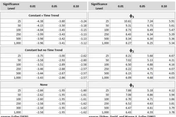
a) We compare the t statistic corresponding to the coefficient , and the ∅ statistic to test = = . The critical values are according to Dickey and Fuller (1976) and Mackinnon (1991). If the null hypothesis is rejected, the test ends. However, if the null hypothesis is not rejected, either the series will have a unit root or the test has insufficient power due to the inappropriate inclusion of a superfluous deterministic regressor;
b) It is suggested to exclude the deterministic trend from the regression, however this is valid only if = . The ∅ statistic evaluates whether = = = . If the null hypothesis is rejected, the procedure ends by accepting the unit root hypothesis;
the coefficient , and the ∅ statistic to test = = . If the null hypothesis is rejected, the procedure ends;
d) If the null hypothesis is not rejected, it could be, for instance, that the power of the test is distorted by not including the constant and trend in the regression. Thus, it is important to verify the t statistic corresponding to the coefficient . If the null hypothesis is rejected, we conclude that there is no unit root in our series
The procedures above conform to the chart below provided by Enders (2009):
Chart 4 – A procedure to test for unit roots
Source: Enders (2009)
4.3.2Unrestricted Cointegrating VAR Model Test
After concluding the unit-root tests, we select the currencies in which both the realized (actual) and fundamental exchange rates are I(1). This is a requirement to test for cointegration. But, why are we going to test for cointegration? Or, a pertinent preceding question is: what is cointegration anyway? Cointegration can be used to assess the
co-movement of two or more series’ trajectories, such as, for instance, those of a long-term asset price and a structural model. The chart below is an attempt to graphically represent the co-movements of two series by the pairs of arrows. Notice that sometimes there is a significant distance between the trajectories. That could translate into larger forecast errors, or
not-so-“good” forecasts. Cointegration is not concerned with the magnitude of forecast errors. It captures something different: both series tend to move in the same direction, even when the movements seem to be erratic and the paths may not be close to each other. Thus, it is
possible that the predicted exchange rates are not “good” forecasts, but that does not mean they are completely unconnected to the actual exchange rates. It is possible that there are
“forces” that coordinately drive both series.
Chart 5 – Graphical example of two cointegrated series
The above explanation is a gentle introduction to cointegration. In the remainder of this section we formally – and not so gently – describe the unrestricted cointegration test we used in our study. We specifically conducted bivariate Johansen tests, per currency, between the actual and predicted exchange rates that are I(1). We describe the multivariate cointegration analysis proposed by Johansen below according to Marçal (1998).
Suppose the unrestricted VAR model is represented by:
� = � �− + � �− + … + �k�− + Φ + , = , … , (12)
Where is a vector of Gaussian errors with zero average and � variance,
represents all the model’s deterministic variables (e.g., constant, trend, etc…), and = − � − � − … − � 1. Assuming all variables are I(1), when we differentiate the process, we end up with the stationary process below:
∆� = � ∆� + … + �k∆� − + Φ + �− + , = , … , ,
� = − ∑= + �, and = −[ − � + … + � ] = −
(13)
The short run dynamics is represented by the matrices � = , … , , while matrix
expresses the variables’ long run dynamics. In order to determine the number of cointegrated
vectors in , it is necessary to determine the order of integration and whether cointegration among variables exists.
Defining as the rank of , the following situations can occur:
a) = , in this case we conclude that all variables are I(1) and that there is no cointegration among them;
b) has a full rank, in this case we conclude that all variables are stationary;
c) < < , matrix has a rank greater than zero and lesser than p (number of variables in the system). In this case, we conclude that there is cointegration among the variables. It is indicated to impose restrictions in the VAR model, that is, a vector error correction model (VEC) is appropriate.
In the last case above, it is possible to define matrix as = ′, where represents the cointegrating vectors, and represents the weight of each cointegrating vector in the
model, or the errors’ speed of adjustment.
Johansen and Juselius (1992) and Johansen (1996) indicates the following procedure to estimate the matrix by likelihood method. Defining = ∆�− , … , ∆�− + , , regress ∆� and �− against . We need additional definitions: and are the residues from these two regressions, and = − ∑�
= ′; , = , is the matrix that
contains the residues’ covariance. It is possible estimate regressing against , this is equivalent to maximize the following likelihood function:
L = − ( ) |�| − ( ) ∑ + ′ ′�− + ′
�
=
(14)
The likelihood function assumes the form of the following regression:
= α ′ + (15)
Two tests are proposed based on the above likelihood function. The first is the trace test, which tests the null hypothesis of cointegrating vectors against the alternative hypothesis of cointegrating vectors. The likelihood ratio test for the trace test is shown in the equation below:
= −� ∑ ( − ̂
= +
(16)
The second is the maximum eigenvalue test, which tests the null hypothesis of cointegrating vectors against the alternative hypothesis of + cointegrating vectors. The likelihood ratio test for the maximum eigenvalue test is shown in the equation below:
= −� ln + ̂ (17)
Where ̂ is the estimated th ordered eigenvalue from the ′ matrices.
of lags. According to Alves (2005), there are three widely accepted VAR lag order selection criteria:
Akaike Information Criterion (AIC): − ⁄ + ⁄
Schwarz Information Criterion (SC): − ⁄ + ⁄
Hannan-Quinn Criterion (HQ): − ⁄ + log ⁄
Where K is the number of estimated parameters, is the number of observations, and is the log-likelihood function value.
In our work, we used the AIC as the primary criterion to determine the number of lags. In case we failed to find cointegrating evidence using the lags defined by the AIC, we tested using the lags suggested by the SC and HQ, in this order.
4.3.3Restricted Cointegrating VAR Model - Unitary Elasticity Test
In the preceding section we explained the test we applied in our study in order to determine whether cointegration exists between the actual and forecasted exchange rates. We have not imposed any restrictions. When cointegration exists, it simply means that there is a
“force” that coordinately drives both series. We do not know how “strong”, or relevant, is this “force”.
Cheung and Chinn (1998) proposed an additional, and more stringent, test defined as unitary elasticity. In this test some restrictions will be imposed in the VAR model in order to verify whether a cointegrating vector is consistent with long run unitary elasticity of expectations.
adjustment parameters, or “weights”, in the vector error model, and contains the cointegrating vectors. The unitary elasticity examination is implemented by merely imposing a test to check whether the cointegraing vector, in the case of our bivariate model, is [1 -1], that is = [ − ].
4.4GRANGER CAUSALITY TEST
In addition to the consistency criteria tests proposed by Cheung and Chinn (1998), we believe it is appropriate to exploit the causality framework laid out by Granger (1969). Granger causality does not infer a cause and effect relationship, but whether the contemporary values of a certain series, , can be explained by the lagged values of another series, . In fact, a bivariate Granger causality test can generate four possible outcomes:
a) Granger-causes ; b) Granger-causes ;
c) Both of the above: Granger-causes and, concurrently, Granger-causes ; d) Not of the above.
How is the Granger causality test applicable to our research? We work with two series here: the log-returns of actual and forecasted exchange rates. A reasonable inspection in the context of our work, for instance, is to test whether the fundamental model, embodied by its forecasts, anticipates the actual returns. We test the causal analysis for a bivariate VAR for our two stationary series. Conveniently, Hamilton (1994) precisely describes Granger causality for such a model. Thus, we will base our explanation about Granger causality, in the remainder of this section, on his work.
[ ] = [ ] + [∅
∅ ∅ ] [
− − ] + [
∅
∅ ∅ ] [
−
− ] +...
+ [∅
∅ ∅ ] [
−
− ] + [ ]
(18)
From the first row of this system, the optimal one-period-ahead forecast of is contingent only on its lagged values (as mentioned before, in this example, plays no role in it):
̂ + | , − , … , , − , … = + ∅ + ∅ − +. . . +∅ − + (19)
Analogously, the value of + is determined by:
+ = + ∅ + + ∅ +. . . +∅ − + + , + (20)
In the example above, it has been imposed that the lagged values of do not contribute to the one-period-ahead forecast of . Now, how would we set the econometric tests for Granger causality? From the autoregressive specification (18), we can implement the following test, assuming a particular autoregressive lag length :
= + − + − +. . . + − + − + − +. . . + − + (21)
We want to test whether the lagged values of play a role in the one-period-ahead forecast of . The null hypothesis is : = =. . . = = .
In order to conclude the Granger causality test, we calculate the following:
S ≡ − (22)
where
= ∑ ̂ �
=
(23)
= ∑ ̂ �
=
(24)
We would conclude the test by comparing the calculate value to the 5% critical values for a variable: we reject the null hypothesis that does not Granger-cause if is greater than the 5% critical value for a variable.
5 RESEARCH METHODOLOGY
5.1RESEARCH HYPOTHESES
The hypothesis formulation and testing procedure allows for the verifiability of the answers to the questions proposed by a study. In our research, we propose to answer the following questions pertinent to the out-of-sample forecasts generated by the model we implement:
Question 1 Is there a difference in predictive accuracy between the log-returns of forecasts generated by the random walk and those of the structural model?
HOQ1: there is no difference in the models’ predictive accuracy.
H1Q1: otherwise.
Question 2 Are the fundamental model predictions consistent, or rational, according to the framework laid out by Cheung and Chinn (1998)? In order to answer this question, we need to verify the following three criteria:
Criterion 1 Do the forecast and the actual exchange-rate series have the same order of integration?
H0Q2C1 both series’ data-generating processes are difference-stationary, I(1).
H1Q2C1 otherwise.
If the null hypothesis is rejected, we conclude the answer to question 2 is negative. Otherwise, we proceed to validate criterion 2.
Criterion 2 Are the series (unrestrictedly) cointegrated? H0Q2C2 the series are not cointegrated.
If the null hypothesis is rejected, we proceed to validate criterion 3. Otherwise, we conclude the answer to question 2 is negative.
Criterion 3 Do the forecast and the actual exchange-rate series have a cointegrating vector consistent with long-run unitary elasticity of expectations? H0Q2C3 there is a linear constraint in the cointegraing vector, = [ − ].
H1Q2C3 otherwise.
If the null hypothesis is rejected, we conclude the answer to question 2 is negative. Otherwise, we conclude the fundamental model’s forecasts are
consistent.
Question 3 Is there a linear serial relation between the log-return of the forecast and the actual exchange-rate series? Or, more specifically, does the structural model, embodied by forecasted returns, anticipate the actual exchange rate?
HOQ3: there is no linear relation between the forecast and the actual exchange-rate returns. The structural model’s forecasted returns do not anticipate those of the actual exchange rates, or vice versa.
H1Q3: there is a persistent linear relation between the structural model's forecasts and
the exchange rate, and the structural model’s forecasts Granger-cause the actual exchange rate returns.
H2Q3: there is a persistent linear relation between the structural model's forecasts and
the exchange rate, and the actual exchange-rate returns Granger-cause those predicted by the structural model.
5.2DATA AND SAMPLE SELECTION
followed the main elements of the inflation-targeting framework during most of the sample period. Unlike Galimberti and Moura (2012), we added industrialized economies to the country list. Thus, our country sample contains both developed and developing countries, namely Brazil, Canada, Chile, the Czech Republic, Hungary, Iceland, Japan, Mexico, Norway, Peru, Poland, South Africa, Sweden, and the United Kingdom. We defined the United States as our benchmark country; thus, we gathered macroeconomic data from this country as well.
The data-collection period ranges from January 1995 to March 2014. Through rolling regressions of a fixed size of 60 periods (months), we were able to generate an unbalanced panel of one-month-ahead monthly exchange-rate forecasts from January 2000 to March 2014. Thus, for each country, we were able to pair the forecast series with the actual exchange rate. The output of the rolling regressions enabled us to obtain an unbalanced panel that is both recent enough to arrive at contemporarily meaningful results and sufficiently extensive to adequately perform our tests. The panel is an unbalanced one because we were not able to generate the first forecast for January 2000 due to the lack of data for some countries.
All data used in our work were extracted from the IMF’s International Financial
Statistics (IFS) database.2 Below we list the IFS line code and the description of the data:
line 00RF: monthly averages of daily quotations of the exchange rates;3
line 64: inflation, as measured by the consumer price index (CPI);
line 66: seasonally adjusted industrial production index (IPSA), used as a proxy for GDP;
line 60B: “call money rate,” used as a proxy for short-term interest rates periodically set by central banks.
The data above are in their “raw” form. To give “life” to our variables, we had to
transform them. We specifically followed the transformations defined by Galimberti and Moura (2012). Where applicable, we explain the proxies used for the variables. These are the same proxies as defined in Molodtsova and Papell (2009) and Galimberti and Moura (2012). The chart below discloses the transformations done in our work.
Chart 6 – Variables transformation
Variable Transformation Where
∆ log( + ⁄ is the average exchange rate (non-U.S. currency per U.S.
dollar)
log ⁄ − CPIinflation. is the consumer price index. It is used as a proxy for
log ⁄ )
The formula represents the output gap, where the IPSA is the seasonally adjusted industrial production, which is used as a proxy for output. The � represents the potential output, calculated by the Hodrick-Prescott filter.
− log + As per Molodtsova and Papell's (2009) money rate” is used as a proxy for the nominal interest rate. convention the “call
Source: developed by the author
We have omitted until now the fact that we used the variables in their logarithmic form. The benefits of using the natural logarithmic form are twofold:
a) The variables assume a non-dimensional form, thus avoiding differences in scale between them;
b) The monthly asset returns can be conveniently added when the returns are continuously compounded. Thus, if we want to accumulate the returns, we can do so simply by adding them.
It is important to mention that for the consistency test, we compare the log-level of the predicted exchange rates to the actual ones.4 We arbitrarily re-scale the series by defining that both the forecasted and the actual exchange-rate series start at zero before the first available forecast. We justify this by arguing that it provides a better graphical visualization with no loss in data properties. We can, for instance, visualize how far apart the forecasted exchange rate is from the actual one during the period analyzed, assuming they started at the same point.
6 EMPIRICAL RESULTS
In this section we report the findings of the tests performed. We answer the questions proposed by our work and provide the evidence to support our conclusions. The table below offers a short roadmap for the remainder of this section.
Chart 7 – Roadmap to the implemented tests
Source: developed by the author
6.1DESCRIPTIVE STATISTICS
Before we present the test results, we think it is illustrative to provide some descriptive statistics pertaining to the fundamental model’s forecasts. The goal here is twofold:
a) To allow a visual inspection of how the structural model’s forecasts follow the
actual exchange rates;
To address the first item, we provide the graphs containing the forecasted and actual exchange-rate series. We define the scale as the log-level of the exchange rates, arbitrarily specifying that both series started at the same point (zero) in the beginning of our forecast sample period. The purpose of the graphs is to provide a visual tool to help answer the question of how well the forecast follows the actual exchange rates. For instance, do the forecasted exchange rates appreciate when the actual ones do? The graphs in Appendix IV provide the tools to informally examine such a question.
We perform the following exercise to address the second item. Suppose we travel back in time and just gather the data to provide our first forecasts based on the Taylor rule model implemented in our work. We run our first regression on each currency subject to our study and review its outputs in order to answer basic questions: Is the model, when applied to each of the currencies, biased? Are the independent variables significant to the model?
Here we essentially want to know how well our model explains the ex-post reality, a
prior exercise we would undertake before using the model to forecast. If the model cannot adequately explain the past, why would we expect it to explain the future? Appendix V
6.2ANSWER TO QUESTION 1–PREDICTIVE ACCURACY TEST RESULTS
In this section we analyze the output of the asymptotic versions of the DM and CW tests reported in the table below:
Table 1 – Diebold-Mariano and Clark-West asymptotic tests results
We can see from Table 1 above that the tests lead to strikingly different conclusions. The DM tests did not find any evidence of predictive-accuracy difference between the structural model and random-walk forecasts. However, for the CW test, for nine out of the fourteen currencies reported there was predictive-accuracy difference between the models,
favoring the fundamental model’s accuracy.
Which of the tests above reports the correct conclusion? Well, according to Rogoff and Stavrakeva (2008), neither of the tests, in their asymptotic versions, is adequate to answer the question about superior predictive accuracy. As pointed out before, the distributional properties of the MSPE's loss function require more robust tests. In Appendix II we provide a
possible methodology to address the asymptotic tests’ shortcomings. However, this suggested methodology uses a VEC model, which requires the series’ cointegration. We will show in the
following sections that cointegration is not always achieved.
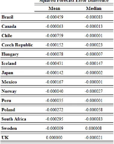
Table 2 – Squared forecast error differences
Source: developed by the author
From the table above we can see that the random walk outperforms the fundamental model in thirteen out of fourteen currencies from the listed countries. The structural model only outperforms the random walk for the British pound (when we consider the mean) and the Swedish krona (when we consider the median).
6.3ANSWER TO QUESTION 2–FORECAST CONSISTENCY TEST RESULTS
6.3.1Criterion 1 – Augmented Dickey-Fuller Test Results
The table below shows the output of the augmented Dickey-Fuller tests. The purpose of this test is to identify the series that are eligible for the cointegration tests. In our case, we
Table 3 – Unit root test results
Table 3 – Unit root test results
(conclusion)
Source: developed by the author. Column U.R. (unit root) specifies the whether the series has a unit root according to the test procedure. * indicates significance at 5%, † specifies that the test procedure conclusion was overruled by graphical evidence, and I(1) indicates the
currency’s series are eligible for cointegration testing. f indicates the forecasted series.
6.3.2Criterion 2 –Unrestricted Cointegration Test Results
Based on the unit root test results, we tested for cointegration for each pair of series that qualified for it. In other words, we tested for cointegration all I(1) forecasts and actual exchange rates. The table below reports the results of the tests.
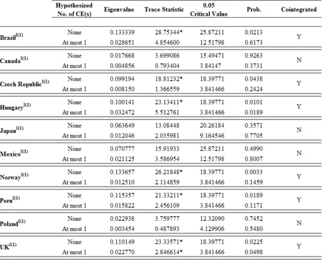
Table 4 – Cointegration test results
Source: developed by the author. * indicates cointegration at 5% significance level.
Verification of Criterion 2: Based on the information above, we conclude that the forecasted and actual series are cointegrated in the currencies of the following countries: Brazil, Czech Republic, Hungary, Norway, Peru, and the U.K. That is, we reject the null
6.3.3Criterion 3–Restricted Cointegrating VAR – Unitary Elasticity Test Results
We test for unitary elasticity all pairs of series that indicated cointegration. This is a more stringent test, following Cheung and Chinn (1998). The table below reports the test results.
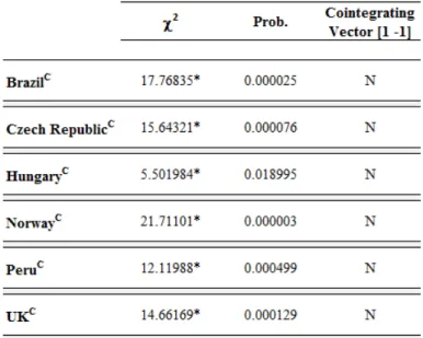
Table 5 – Unitary elasticity test results
Source: developed by the author. C indicates series unrestrictedly cointegrated (as per previous test), and * rejects the null hypothesis that the cointegrating vector is [1 -1] at 5% significance.
Verification of Criterion 3: Based on the information above, we reject the null hypothesis of long-run unitary elasticity of expectations for all tested currencies.
6.4ANSWER TO QUESTION 3-GRANGER CAUSALITY TEST RESULTS
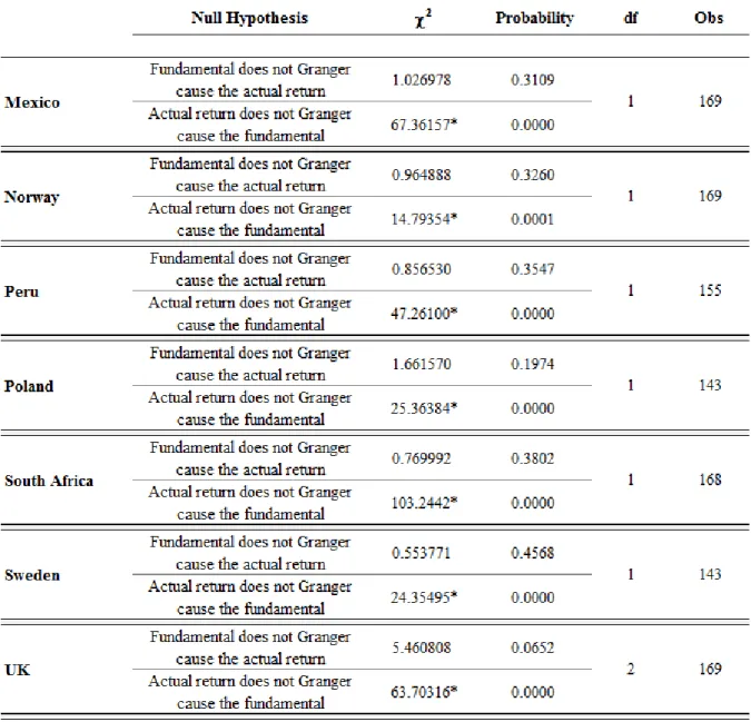
The table below shows the results for the Granger causality tests. Table 6 – Granger causality test results log-returns of exchange rates
Table 6 – Granger causality test results - log-returns of exchange rates
(conclusion)
Source: developed by the author. * indicates Granger causality at 5% significance.
Answer to Question 3: Based on the results above, none of the forecasted series, expect for the Japanese Yen, was able to Granger-cause the actual exchange rates.
Surprisingly, for all of the countries’ currencies the actual return Granger-caused the
7 CONCLUSION
Our work thoroughly investigates whether Molodtsova and Papell’s (2009)
“symmetric Taylor rule model with heterogeneous coefficients, smoothing, and a constant”
generates out-of-sample forecasts that
a) provide better predictive accuracy than those of a random walk;
b) are consistent, or rational, according to the framework laid out by Cheung and Chinn (1998);
c) anticipate the actual exchange rates.
Overall, the results are not favorable to the implemented structural model. Coldly reporting the results, we find no evidence of better forecast accuracy or consistency, nor do we find that the forecast series anticipate actual exchange rates. Does it mean that the model yields forecasts completely unconnected to actual exchange rates? The answer is no. In six of the fourteen currencies analyzed, we found that the forecast series cointegrated with the actual ones. This means that, in almost half of our currency sample, the structural model proved to
be an eligible “force” acting on the exchange rate.
Thinking about Taylor rule models more broadly, we consider that we should not be totally discouraged about their role in exchange-rate forecasting. The Taylor rule model we implemented can be improved. The Molodtsova and Papell (2009) model is a backward-looking model, that is, it does not account for expectations. An expectation-based Taylor rule model is proposed by Engel, Mark, and West (2007), who reported encouraging results by bringing expectations into the model. However, we cannot forsake Rogoff and Stavrakeva’s
(2008) well-founded skepticism about the predictive ability of fundamental models. It is important to apply robust tests over different sample periods: the model may perform well over a period but poorly over a different section of the sample.
a) The model could benefit from asset-pricing theory and additional explanatory variables. Some of these variables, such as risk premium, may not be observed but may be very relevant, and could be incorporated to a Taylor rule-based model; b) The forecast evaluation methodology can be improved by implementing residual
bootstrap techniques in the cointegrated series. This could enhance the robustness of the forecast accuracy tests.
We conclude our work with the same paradoxical feelings we had before we started. On one hand, it seems tremendously naïve to believe one can build a model capable of decently forecasting exchange rates: if such a model were discovered, what would happen when it became available to all? Attempting to answer such a question leads to absurd responses. On the other hand, from a scientific perspective, it seems lazy not trying to improve exchange rate models. Our role as scientists is to indefatigably explain the unexplainable, leaving the least as possible to randomness. In pursuing enlightenment to a phenomenon, it is sluggish to attribute to chance what can be explained.