© 2013 Science Publications
doi:10.3844/jmssp.2013.65.71 Published Online 9 (1) 2013 (http://www.thescipub.com/jmss.toc)
FORECASTING THE FINANCIAL RETURNS
FOR USING MULTIPLE REGRESSION
BASED ON PRINCIPAL COMPONENT ANALYSIS
Nop Sopipan
Program of Mathematics and Applied Statistics, Faculty of Science and Technology, Nakhon Ratchasima Rajabhat University, Nakhon Ratchasima, Thailand
Received 2012-08-30, Revised 2013-01-11; Accepted 2013-04-17
ABSTRACT
The aim of this study was to forecast the returns for the Stock Exchange of Thailand (SET) Index by adding some explanatory variables and stationary Autoregressive order p (AR (p)) in the mean equation of returns. In addition, we used Principal Component Analysis (PCA) to remove possible complications caused by multicollinearity. Results showed that the multiple regressions based on PCA, has the best performance.
Keywords: SET Index, Forecasting, Principal Component Analysis, Multicollinearity
1. INTRODUCTION
In order to forecast the return rt for specific purposes, many researchers have made different assumptions for µt as appears in Equation (2). Kyimaz and Berument (2001) assume µt to be a regression model with a one-week delay; Supoj (2003) assumes µt to be an autoregressive process; Ozturk (2008) assumes µt to be a constant and Sattayatham et al. (2012) assume µtto be an ARMA process with a one-week delay.
The financial returns rt (r = 100 × ln(P / P )t t t -1 for t = 1,2,…,T-1, Pt denoting the financial price at time t depend concurrently and dynamically on many economic and financial variables. Since the returns have a statistically significant autocorrelation themselves, lagged returns might be useful in predicting future returns. In order to model these financial returns ssumes that rt follows a simple time series model such as a stationary AR (p) model with some explanatory variables Xit. In other words, rt satisfies the following Equation 1:
t t t
p n
t 0 i it j t - j i =1 j=1 r = +ε ,
ε = +
∑
αX +∑
βr , (1)Where Equation 2:
it it
i( t 1)
P
X 100 ln( )
P −
= ⋅ (2)
Here Pit denotes the financial price asset i for i = 1,2,…,n at time t, rt-j, j = 1,2,….,pis the returns at lag j-th, εt represents errors assumed to be a white noise series with an i.i.d. mean of zero and a constant variance 2
ε
σ , µ0,αi and βj are constants and n, p are positive integers.
Note that the variance of errors εt in the model (2) is assumed to be a constant; some authors use this assumption in the modeling of ground-level ozone (Agirre-Basurko et al., 2006; Pires et al., 2008).
The objective of this study is to forecast returns for the SET Index by using model (1). We vary the process µt using four different types and compare the performance of the different types.
2. PRINCIPAL COMPONENT ANALYSIS
An important topic in multivariate time series analysis is the study of the covariance (or correlation) structure of the series. For example, the covariance structure of a vector return series plays an important role in portfolio selection. In what follows, we discuss some statistical methods useful in studying the covariance structure of a vector time series.
Given a m-dimensional random variable
t 1t 2t nt t-1 t-p
R = (X ,X ,...,X ,r ,...,r )' with covariance matrix ∑R,
a Principal Component Analysis (PCA) is concerned with using a few linear combinations of Rt to explain the structure of ΣR. If Rf denotes the monthly log returns of m assets, then PCA can be used to study the source of variations of these m asset returns. Here the keyword is few so that simplification can be achieved in multivariate analysis.
PCA applies to either the covariance matrix ΣR
R
∑ or the correlation matrix (ρR) of Rf. Since the correlation matrix is the covariance matrix of the standardized random vector * -1
t t
R = S R , where S is the
diagonal matrix of standard deviations of the components of Rt, we use covariance matrix in our theoretical discussion. Let δi =(δi1,...,δim) 'be a m-dimensional vector, where I = l,…m.
Then Zit= δi'R= δij
j=1 m
∑
Rjt is a linear combination ofthe random vector Rt. If Rt consists of the simple returns of m stocks, then Zit is the return of a portfolio that assigns weight δij to the jth stock. Since multiplying a constant to δi does not affect the proportion of allocation assigned to the jth stock, we standardize the vector δi so that
m
' 2
i i ij j=1
δ δ =
∑
δ = 1. Using properties of a linearcombination of random variables, we have
Var(Zit)= δi
'Σ
Rδi, Cov(Zit, Zjt) =δi
'∑
Rδj,for i,j = 1,2,…,m.
The idea of PCA is to find linear combinations δi such that Zit and Zjt are uncorrelated for i≠j and the variances of Zit are as large as possible. More specifically:
• The first principal component of Rt is the linear combination Z1t= δ1
'
Rt that maximizes Var(Z )1t subject to the constraint '
1 1
δ δ = 1.
• The second principal component of R is the linear
combination '
2t 2 t
Z =δR that maximizes Var(Z )2t
subject to the constraints ' 2 2
δ δ = 1 and
Cov(Z1t, Z2t) = 0.
• The ith principal component of R is the linear combination Zit =δi
'
Rt that maximizes Var(Z )it subject to the constraints '
i i it jt
δ δ = 1 and Cov(Z , Z ) = 0
for j = 1,...,i -1
Since the covariance matrix ΣR is non-negative definite, it has a spectral decomposition. Let
1 1 m m
(λ,e ),...,(λ ,e ) be the eigenvalue-eigenvector pairs of
ΣR, where λ1³λ2³ ... ³λm³ 0. We have the following statistical result as follow: The ith principal component
of ris Zit=e'i
Rt = eij
j=1 m
∑
Rjt for i = l,…,m Moreover:'
it i R i i ' it jt i R i
Var(Z ) = e e = , i = 1,..., m,
Cov(Z , Z ) = e e = 0, i j
∑
∑ ≠
λ
If some eigenvalues λiare equal, the choices of the corresponding eigenvectors ei and hence Zit are not
unique. In addition, we have
V ar(Rit) i=1 m
∑
= tr(∑R) = λi
i=1 m
∑
= V ar(Zit) i=1m
∑
.The result says that:
it i
m
1 m
it i=1
Var(Z ) λ
=
λ + ... +λ
Var(Z )
∑
Consequently, the proportion of total variance in Rt explained by the ith principal component is simply the ratio between the ith eigenvalue and the sum of all eigenvalues of ΣR. One can also compute the cumulative proportion of total variance explained by the first i principal components (i.e., j=1λj
i
∑
/∑
mj=1λj). In practice, one selects a small i such that the prior cumulative proportion is large.In order to cope with the problem of multicollinearity, we transform the explanatory variables in model (1) into the principal components. Then the new model for forecasting rt is Equation 3:
m
t 0 i it t i =1
r = +
∑
αZ +ε, (3)We follow Tsay (2005) by assuming that the asset return series rt is a weekly stationary process.
3. EMPIRICAL STUDIES AND
METHODOLOGY
Naturally, the Thai stock market has unique characteristics, so the factors influencing the price of stocks traded in this market are different from the factors influencing other stock markets (Chaigusin et al., 2008). Examples of factors that influence the Thai stock market and the statistics used by researchers who have studied these factors in forecasting the SET Index are shown in Table 1.
3.1. Data
The data sets used in this study are the daily return closing prices for the SET Index at time t (dependent variables) and the daily return closing prices for twelve factors (explanatory independent variables).
These twelve factors are the following: • The Dow Jones Index at time t-1 (DJIA)
• The Financial Times 100 Index at time t-1 (FSTE) • The S&P 500 Index at time t-1 (SP)
• The Nikkei225 Index at time t (NIX) • The Hang Seng Index at time t (HSKI)
• The Singapore Straits Times Industrial Index at time t (SES009)
• The Taiwan Stock Weighted Index at time t (TWII) • The South Korea Stock Exchange Index at time t
(KOSPI)
• The Oil Price in the New York Mercantile Exchange at time t (OIL)
• The Gold Price in the New York Mercantile Exchange at time t (GOLD)
• The Currency Exchange Rate in Thai Baht for one US dollar at time t (THB/USD)
• The Currency Exchange Rate in Thai Baht for one Hong Kong dollar at time t (THB/HKD)
The actual closing prices for these twelve factors were obtained from http://www.efinancethai.com. We used data sets from April 5, 2000, to July 5, 2012. We divided these data into two disjoint sets. The first set, from April 5, 2000, to December 30, 2011, was used as a sample (2,873 observations). The second set, from January 3, 2012, to July 5, 2012, was used as out-of-sample (125 observations). The plot for the SET Index closing prices and returns is given in Fig. 1.
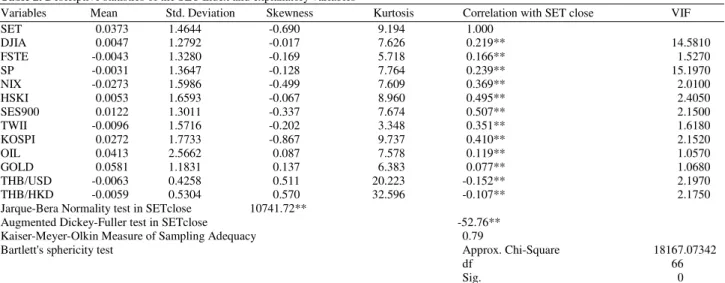
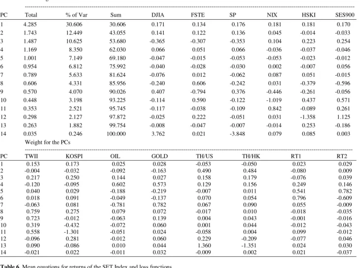
Descriptive statistics and the correlations matrix are given in Table 2 and 3. As can be seen from Table 3, there are highly significant correlations (p<0.01) between the dependent variables and the explanatory variables. Therefore, these explanatory variables were used to predict the SET Index. Also, there are highly significant correlations (p<0.01) among the explanatory variables. From Table 4 there are significant correlations between SET and lagged returns of the SET with first and second laggs. These correlations provide a measure for the linear relations between two variables and also indicate the existence of multicollinearity between the explanatory variables. However, multiple regression analysis based on this dataset also shows that there was a multicollinearity problem with the variance inflation factor (VIF> = 5.0) as shown in Table 2. One approach to avoid this problem is PCA. Hence, we used twelve explanatory variables to find the principal components and overall descriptive statistics for selected Principal Components (PCs), as shown in Table 5 and 6, respectively.
Table 1. Impact factors on the Stock Exchange of Thailand Index (SET Index)
Factors Researchers
---
1 2 3 4 5 6 7 8
The Nasdaq Index X
The Down Jones Index X X X X X X X X
The S&P 500 Index X
The Nikkei Index X X X X X X
The Hang Seng Index X X X X X X
The Straits Times Industrial Index X X X
The Currency Exchange Rate in Thai Baht to one US dollar X X X X
The Currency Exchange Rate in Thai Baht to 100 Japan Yen X X
The Currency Exchange Rate in Thai Baht to one Hong Kong dollar X
The Currency Exchange Rate in Thai Baht to one Singapore dollar X
Gold Prices X X X
Oil Prices X X X
Minimum Loan Rates X X X X X
Fig. 1. Graph of the SET Index (a) and returns of the SET Index (b)
3.2. Results of Principal Component Analysis
Bartlett’s sphericity test for testing the null hypothesis where the correlation matrix is an identity matrix was used to verify the applicability of PCA. The value of Bartlett’s sphericity test for the SET Index was 18,167.07, which implies that the PCA is
Table 2. Descriptive statistics of the SET Index and explanatory variables
Variables Mean Std. Deviation Skewness Kurtosis Correlation with SET close VIF
SET 0.0373 1.4644 -0.690 9.194 1.000
DJIA 0.0047 1.2792 -0.017 7.626 0.219** 14.5810
FSTE -0.0043 1.3280 -0.169 5.718 0.166** 1.5270
SP -0.0031 1.3647 -0.128 7.764 0.239** 15.1970
NIX -0.0273 1.5986 -0.499 7.609 0.369** 2.0100
HSKI 0.0053 1.6593 -0.067 8.960 0.495** 2.4050
SES900 0.0122 1.3011 -0.337 7.674 0.507** 2.1500
TWII -0.0096 1.5716 -0.202 3.348 0.351** 1.6180
KOSPI 0.0272 1.7733 -0.867 9.737 0.410** 2.1520
OIL 0.0413 2.5662 0.087 7.578 0.119** 1.0570
GOLD 0.0581 1.1831 0.137 6.383 0.077** 1.0680
THB/USD -0.0063 0.4258 0.511 20.223 -0.152** 2.1970
THB/HKD -0.0059 0.5304 0.570 32.596 -0.107** 2.1750
Jarque-Bera Normality test in SETclose 10741.72**
Augmented Dickey-Fuller test in SETclose -52.76**
Kaiser-Meyer-Olkin Measure of Sampling Adequacy 0.79
Bartlett's sphericity test Approx. Chi-Square 18167.07342
df 66
Sig. 0
**Significant at the 0.01 level (2-tailed)
Table 3. Correlation matrix of the SET Index and explanatory variables
Correlations SET DJIA FSTE SP NIX HSKI SES900 TWII KOSPI OIL GOLD THB/USD THB/HKD
SET 1.00
DJIA 0.22** 1.00
FSTE 0.17** 0.55** 1.00
SP 0.24** 0.96** 0.56** 1.00
NIX 0.37** 0.45** 0.39** 0.47** 1.00
HSKI 0.50** 0.37** 0.29** 0.40** 0.59** 1.00 SES900 0.51** 0.33** 0.20** 0.35** 0.53** 0.70** 1.00 TWII 0.35** 0.30** 0.23** 0.32** 0.45** 0.49** 0.47** 1.00 KOSPI 0.41** 0.31** 0.26** 0.34** 0.59** 0.61** 0.57** 0.57** 1.00 OIL 0.12** 0.01 -0.01 0.01 0.06** 0.10** 0.11** 0.06** 0.06** 1.00 GOLD 0.08** 0.04* 0.03 0.05** 0.07** 0.09** 0.07** 0.02 0.07** 0.20** 1.00 THB/USD -0.15** -0.07** -0.05** -0.08** -0.08** -0.12** -0.12** -0.10** -0.13** -0.04* -0.13** 1.00
THB/HKD -0.11** 0.00 -0.01 -0.02 0.00 -0.07** -0.10** -0.11** -0.08** -0.12** -0.02 -0.10** 1.00 **Correlation significant at the 0.01 level (2-tailed)
Table 4. Correlation matrix of the SET Index and lagged returns of the SET
Correlations SET SETt-1 SETt-2 SETt-3 SETt-4
SET 1.00
SETt-1 0.036* 1.00
SETt-2 0.073** 0.036* 1.00
SETt-3 0.007 0.073** 0.036* 1.00
SETt-4 -0.018 0.007 0.073** 0.036* 1.00
*,**Correlation significant at the 0.05, 0.01 level (2-tailed) respectively.
4. FORECASTING THE RETURNS THE
SET INDEX BY MEAN EQUATIONS
In this section, we forecast the returns for the SET Index (rt := µt + εt) using three mean equations (µt): constant, AR (2) and multiple regression based on PCA. Afterwards, we compare error using two loss functions, i.e. Mean Square Error (MSE) and Mean
Table 5. Descriptive statistics of selected PCs Initial Eigenvalues
---
PC Total % of Var Sum DJIA FSTE SP NIX HSKI SES900
1 4.285 30.606 30.606 0.171 0.134 0.176 0.181 0.181 0.170
2 1.743 12.449 43.055 0.141 0.122 0.136 0.045 -0.014 -0.033
3 1.487 10.625 53.680 -0.365 -0.307 -0.353 0.104 0.223 0.254
4 1.169 8.350 62.030 0.066 0.051 0.066 -0.036 -0.037 -0.046
5 1.001 7.149 69.180 -0.047 -0.015 -0.053 -0.053 -0.023 -0.012
6 0.954 6.812 75.992 -0.040 -0.028 -0.030 0.002 -0.007 0.056
7 0.789 5.633 81.624 -0.076 0.012 -0.062 0.087 0.051 -0.015
8 0.606 4.331 85.956 -0.240 0.606 -0.242 0.031 -0.379 -0.596
9 0.570 4.070 90.026 0.407 -0.794 0.376 -0.446 -0.261 -0.056
10 0.448 3.198 93.225 -0.114 0.590 -0.122 -1.019 0.437 0.571
11 0.353 2.521 95.745 -0.117 -0.038 -0.109 0.842 -0.089 0.261
12 0.298 2.127 97.872 -0.025 0.222 -0.051 0.031 -1.358 1.125
13 0.263 1.882 99.754 -0.008 -0.047 -0.007 -0.014 0.253 -0.186
14 0.035 0.246 100.000 3.762 0.021 -3.848 0.079 0.085 0.003
Weight for the PCs
---
PC TWII KOSPI OIL GOLD TH/US TH/HK RT1 RT2
1 0.153 0.173 0.025 0.028 -0.053 -0.050 0.023 0.029
2 -0.004 -0.032 -0.092 -0.163 0.490 0.484 -0.080 0.009
3 0.217 0.250 0.144 0.027 0.158 0.179 -0.076 0.039
4 -0.120 -0.095 0.602 0.573 0.129 0.156 0.249 0.146
5 0.040 0.029 -0.188 -0.219 -0.007 0.011 0.541 0.782
6 0.018 0.091 -0.049 -0.137 0.070 0.054 0.796 -0.609
7 -0.063 0.081 -0.781 0.782 0.067 0.090 0.055 -0.009
8 0.759 0.275 0.079 0.072 -0.017 0.010 -0.018 -0.035
9 0.723 -0.012 -0.063 0.139 0.004 0.043 -0.001 -0.016
10 0.319 -0.432 -0.072 0.060 0.001 0.044 -0.012 -0.043
11 0.558 -1.301 -0.051 0.024 -0.058 0.004 0.099 -0.012
12 -0.096 0.281 -0.012 0.060 0.229 -0.209 -0.077 0.046
13 0.090 -0.086 0.010 0.044 1.360 -1.351 0.024 0.030
14 -0.021 0.022 -0.011 0.032 -0.009 0.002 0.021 -0.037
Table 6. Mean equations for returns of the SET Index and loss functions
Model Mean Equation MSE MAE
1. Constant mean. t= E[r ],t t= 0.0373 0.8914 0.7576
2. AR (2) t= 0+α1 t-1r +α2 t-2r , t= 0.34r + 0.72r . t-1 t-2 0.8900 0.7570
3. Multiple regressions based on PCA.
n
t 0 i it
i=1
= +
∑
βZt= 0.718Z - 0.132Z + 0.319Z - 0.14Z + 0.141Z1t 2t 3t 8t 10t- 0.063Z13t 0.8886 0.7463
5. CONCLUSION
We considered the problem of forecasting returns for the SET Index by using a stationary Autoregressive order p (AR (p)) with some explanatory variables. After considering four types of mean equations, we transformed AR and explanatory variables to PC. We found that multiple regressions based on PCA, has the best performance(MSE = 0.8886, MAE = 0.7463).
6. REFERENCES
Agirre-Basurko, E., G. Ibarra-Berastegi and I. Madariaga, 2006. Regression and multilayer perceptron-based models to forecast hourly O3 and NO2 levels in the Bilbao area. Environ. Model.
Software, 21: 430-446. DOI:
Chaigusin, S., C, Chirathamjaree and J. Clayden, 2008. Soft computing in the forecasting of the Stock Exchange of Thailand (SET). Proceedings of the 4th IEEE International Conference on Management of Innovation and Technology, Sept. 21-24, IEEE Xplore Press, Bangkok, pp: 1277-1281. DOI: 10.1109/ICMIT.2008.4654554
Kyimaz, H. and H. Berument, 2001. The day of the week effect on Stock Market Volatility. J. Econ. Finance, 25: 181-193.
Ozturk, M., 2008. Genetic aspects of hepatocellular carcinogenesis. Semin. Liver Dis., 19: 235-242. DOI: 10.1055/s-2007-1007113
Pires, J.C.M., F.G. Martins, S.I.V. Sousa, M.C.M. Alvim-Ferraz and M.C. Pereira, 2008. Selection and validation of parameters in multiple linear and principal component regressions. Environ. Model.
Software, 23: 50-55. DOI:
10.1016/j.envsoft.2007.04.012
Sattayatham, P., Sopipan, N. and B. Premanode, 2012. Forecasting the stock exchange of Thailand uses day of the week effect and markov regime switching GARCH. Am. J. Econ. Bus. Admin., 4: 84-93. DOI: 10.3844/ajebasp.2012.84.93
Supoj, C., 2003. Investigation on Regime Switching in Stock Market. Thammasat University, Bangkok, Thailand.