Escola de Pós-Graduação em Economia - EPGE
Fundação Getulio Vargas
Essays on International Economics
Tese submetida à Escola de Pós-Graduação em Economia da Fundação Getulio
Vargas como requisito de obtenção do Título de Doutor em Economia
Aluna: Ana Lucia Vahia de Abreu
Professora Orientadora: Maria Cristina Trindade Terra
Escola de Pós-Graduação em Economia - EPGE
Fundação Getulio Vargas
Essays on International Economics
Tese submetida à Escola de Pós-Graduação em Economia da Fundação Getulio
Vargas como requisito de obtenção do Título de Doutor em Economia
Aluna: Ana Lucia Vahia de Abreu
Banca Examinadora:
Professora Maria Cristina Trindade Terra (Orientadora, EPGE/FGV)
Professor Afonso Arinos de Mello Franco Neto (EPGE/FGV)
Professor Luiz Renato Regis de Oliveira Lima (EPGE/FGV)
Professora Lia Valls Pereira (UERJ/IBRE)
Professor Gustavo Maurício Gonzaga (PUC/RJ)
Rio de Janeiro
Contents
List of Figures ii
List of Tables iii
Acknowledgements iv
Chapter 1 - Introduction 1
Chapter 2 - Purchasing Power Parity: The Choice of Price Index 3
Chapter 3 - The Relative-factor-endowment as one of the Determinants of the Real Exchange Rate 32
List of Figures
Figure 1 Profit Maximization 51
Figure 2 Pearson Product-Moment Correlation Coefficient for Bilateral RER 52
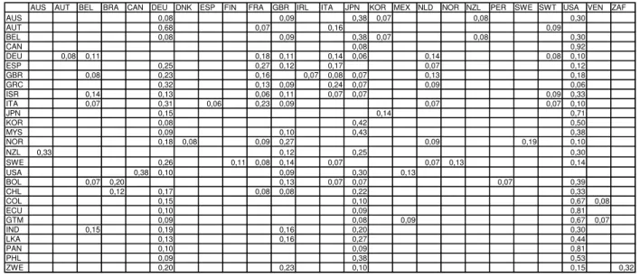
Figure 3 Pearson Product-Moment Correlation Coefficient for Multilateral RER 54
Figure 4 Spearman Rank Correlation Coefficient for Bilateral RER 56
List of Tables
Table 1 ADF and DF-GLS tests: RER based on export unit value 24
Table 2 ADF and DF-GLS tests: RER based on wholesale price index 25
Table 3 ADF and DF-GLS tests: RER based on consumer price index 26
Table 4 ADF and DF-GLS tests: RER based on unit labor costs 27
Table 5 ADF and DF-GLS tests: RER based on normalized unit labor costs 28
Table 6 ADF and DF-GLS tests: RER based on value added 29
Table 7 ADF and DF-GLS tests: RER based on CPI over WPI 30
Table 8 Countries with PPP evidence 31
Table 9 Trade Weights 47
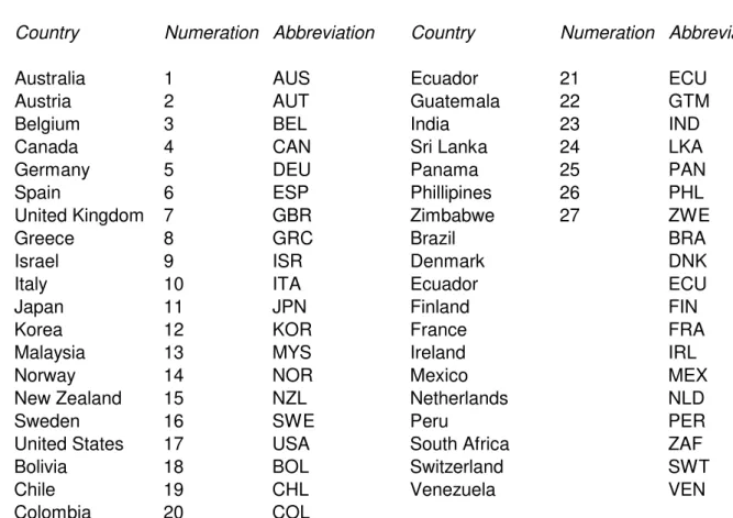
Table 10 Numeration and Abbreviation of Countries 48
Table 11 Average RER Correlations 49
Table 12 DF-GLS Test of the RER 50
Table 13 Nominal and Effective Tariffs 72
Table 14 Labor demand elasticity using employment level as a measure of labor demand 73
Acknowledgements
À orientadora Maria Cristina Terra, pela dedicação e por ter me ensinado muito durante a tese.
Aos amigos de longa data, Fernandinha, Clarice, Denise, Marcos Amaral, Sérgio Brissac, Leopoldo, Ana Paula, Emily, Paulo, Claudinha, Zerbini, Chaon, Monique, Marcelo e Bill, que sempre estiveram ao meu lado.
Às amigas, Lise e Lara, pela incessante torcida durante toda a tese.
Aos amigos da EPGE, Gibinho, Márcia Leon, Márcio Salvato, Marcos Tsuchida, Henrique, Lucas, Genaro, Ângelo, Rebecca, Joísa, Mônica, Silvia, Raffaella, Ricardo Pereira, Osmani e Carlos Hamilton, que tornaram mais suave a árdua caminhada na EPGE.
Aos professores Afonso Arinos e Bernardo Blum, por terem me incentivado a estudar Comércio Internacional e ao professor Fernando de Holanda Barbosa, por ter confiado no meu trabalho. Ao professor Luiz Renato, pelo apoio em econometria.
Aos funcionários da FGV, Regina. Márcia Valéria, Cristina Igreja, Mary, Sônia, Beralda, Sueli, Denise, Ligia, Marcelo, Malaquias, Sandro, Rademaker, Fabrício, Vidal e Dona Margarida, pelo companheirismo.
Aos amigos da Petrobras, Anne, José Luiz, César, Luis Fernando, Jomar, Rogério, Lucymar, Sandra, Álvaro e Leonardo, pela compreensão e companheirismo.
Aos meus pais, por me ensinarem a enfrentar os obstáculos de frente, meu eterno obrigado. Às minhas irmãs e sogra, pela ajuda com os meus filhos.
Chapter 1
Introduction
This study in International Economics has three main goals. First, to indicate, among seven price indices, the one with the highest purchasing power parity (PPP) evidence; second, to suggest that the international trade theory explains to satisfaction the real exchange rate parity among countries with similar relative-factor-endowment; and third, to study the impact of the Brazilian trade openness on labor demand elasticity. Next, we describe the chapters of the thesis.
price index choice to measure the RER.
Chapter three shows, theorically and empirically, that the international trade theory may enhance a new study of the behavior of the RER, de…ned as price of tradable goods over nontradable goods. Starting with a theoretical model which has the RER as a function of relative price factors for a group of countries distributed between two cones of diversi…cation, we show that the realtive-factor-endowment does matter for the behavior of the RER because these endowments determine the subset of tradable goods that the countries produce. Using multilateral and bilateral RER for monthly data from 1985 to 1995 for 27 developing and developed countries, we conclude that the RER is positively correlated among countries in the same cone of diversi…cation and negatively correlated among countries of di¤erent cones of diversi…cation. We endorse our conclusion, doing the PPP testing for bilateral RER for all countries in the sample. The results suggest that the PPP evidence is larger among countries in the same cone of diversi…cation than in di¤erent cones.
Chapter 2
Purchasing Power Parity: The Choice
of Price Index
2.1
Introduction
The purchasing power parity (PPP) hypothesis, in its original formulation, states that the price levels of two countries should be equal, when measured by the same currency. This is an old idea in economics, but the term was coined only in 1918 by Gustav Cassel. As Cassel (1918) puts it, “(a)s long as anything like free movement of merchandise and a somewhat comprehensive trade between the two countries takes place, the actual rate of exchange cannot deviate very much from this purchasing power parity.”
Although ever since some variant of PPP has been the building block for modeling ex-change rates long-run behavior, empirical evidence on its validity is, at best, controversial. PPP does not seem to hold in the short run at all, which …ts economists assessment that PPP should not hold continuously. However, empirical evidence on long run validity of PPP is also scant. The empirical literature on the subject has investigated possible reasons for the failure of …nding hard evidence on long run PPP. Part of the literature credits this failure to the combination of slow speed of convergence, high short run volatility, and not long enough periods of time for testing the long run behavior of the series, for the studies concentrate on post-Bretton-Woods data. The idea is that, with a long enough time span, data on prices and exchange rates would deliver PPP. (See Froot and Rogo¤, 1995, and Rogo¤, 1996.)
PPP (see Sarno and Taylor, 2002, for a brief review of this literature). The problem in covering a long time frame is that it encompasses several di¤erent exchange rate regimes. It would be desirable to limit the sample to the pos-Bretton-Woods period. Long time periods are also more prone to include periods with real shock that shift the equilibrium real exchange rate (RER).
Another strand of literature tries to circumvent the short period of time after Bretton Woods by using panel data. Several such studies reject random walk for the panel. These results, however, solely indicate that random walk is rejected for at least one of the RERs used. They do not provide evidence of PPP holding for all of them. Sarno and Taylor (2002) also discuss the results of this literature.
The literature has also turned to nonlinear models to explain real exchange rate dynamics. The idea is that transaction costs would yield deviations from PPP, which, in turn, would follow a mean reverting nonlinear process. This would also explain PPP deviations for long periods of time. Sarno and Taylor (2002) present a thorough discussion of this evolving line of research.
An old concern about PPP testing, dating back to Keynes (1932), is the very choice of the price indices to be used. The ideal index should measure the exact same basket of goods in all countries, and these goods should all be tradable. Such an index does not exit, though. The most commonly indices used for testing PPP are Consumer Price Index (CPI) and Wholesale Price Index (WPI). A positive feature of these indices is that they are readily available for most countries and for long time frames. On the negative side, these indices include nontradable goods and they do not measure a common basket of goods across countries. The CPI includes a larger share of nontradable goods than the WPI, hence, one could argue, the WPI would better suit the PPP concept.
prices. This paper also tests the stationarity for the RER measured as the relative price of tradable to nontradable goods. That RER is a guideline for the allocation of resources between tradable and nontradable goods. In opposition to the static concept of PPP, that measure of RER may vary in the long run according to its fundamentals.
There are studies that test the PPP hypothesis for di¤erent price indices such as Dornbush (1987) that uses CPI, GDP de‡ator, the GDP de‡ator for manufacturing and export prices of non-electrical machinery for Germany, Japan and US using annual data from 1971 to 1983. He …nds no evidence of PPP for all price indices studied. Chinn (1998) also implements the PPP testing for eight East Asian economies and di¤erent price indices: CPI, PPI and export price index with monthly data from 1970 to 1997. The results suggest some support for the PPP hypothesis when PPI is used. Cheung and Lai (1993) also study the PPP hypothesis using CPI and PPI. Based on the monthly data from January 1974 to December 1989 and …ve countries: UK, France, Germany, Switzerland and Canada, they conclude that for univariate model (real exchange rate), there is no evidence of long run PPP for both price indices. Sarno and Taylor (2002) pointed out that “Also, interestingly, stronger evidence supporting PPP is suggested when the WPI is used rather than the CPI and, even more so, when the GDP de‡ator is used. This is easy to explain since the WPI price level contains a relatively smaller nontradables component and represents, therefore, a better approximation to the ideal price index required by the PPP hypothesis than the CPI and the GDP de‡ator.” The objective of this chapter is to use the larger number of price indices available from IMF for the most number of countries, to yield the one with the highest PPP evidence.
by Elliot and al. (1996). This test is a modi…cation of ADF test that increases its power without otherwise altering the method of testing.
Our main results are the following. First, the RER constructed with WPIs supports the PPP hypothesis for the larger number of countries. Hence, this index seems to be the one that best represents tradable goods with similar basket of goods for all countries. Second, when using export unit values, the PPP is veri…ed for only 4 countries. This index includes only goods that are actually traded by the country, hence its basket of goods composition most probably di¤ers across countries to a greater extent, compared to the other indices. Third, deterministic trends were found to be signi…cant, possibly indicating some Balassa-Samuelson e¤ect. Fourth, for the RER measured as the ratio of foreign CPI and domestic WPI, we …nd no evidence of PPP holding. This is consistent with the idea that CPI has a large share of nontradable goods which are not arbitraged across countries.
The paper is organized as follows. Section two presents the purchasing power parity argument, and its relation to the price indices used to calculate relative purchasing power. The methodology used in the empirical exercises is presented in section three. Section four presents the data and section …ve the empirical results. Finally, section 6 concludes.
2.2
Purchasing Power Parity
Absolute PPP states that, abstracting from any trade frictions, price levels in two economies should be equal, when measured in the same currency, that is:
EP
P = 1; (2.1)
where E is the exchange rate, and P and P are the price indices in home and foreign countries, respectively. In reality, impediments to trade, such as transport costs and trade barriers, prevent prices to be perfectly equalized. Trade restrictions do not preclude prices from being arbitraged, though, so that prices in di¤erent countries should be closely related. Relative PPP allows for obstacles to trade that drive a wedge between the purchasing power of currencies. It states that exchange rate change should re‡ect relative price changes:
b
E =Pb P ;c (2.2)
Going from absolute PPP to relative PPP is not only a way of getting around the qual-i…cations arising from trade frictions. It is also a way to solve the problem of prices that are only reported as indices, as opposed to an actual price for a basket of goods. As price indices are normalized in a base year, even if absolute PPP held, equation (2.1) would not hold.
PPP, in both its absolute or relative versions, depicts a relationship between tradable goods, for these are the goods that are arbitraged by international trade. Hence, the price indices used for testing either equation (2.1) or equation (2.2) should contain only tradable goods. Moreover, the price indices to be compared should be composed of the same basket of goods. Unfortunately, no price index has these two features: available price indices available always contain both tradable and nontradable goods, and its composition of goods varies, not only across countries, but also over time.
To illustrate the e¤ect on PPP testing for the presence of nontradable goods in the price index and of di¤erences in the price indices composition, let us represent domestic and foreign price indices by a weighted average of tradable and nontradable goods:
P =PNPT1 , and P =PN PT(1 );
where PN and PT represent nontradable and tradable goods, respectively, and and
are the share of nontradable goods in domestic and foreign price indices, repectively. The currency purchasing power for these two price indices, that is, the real exchange rate (RER), equals:
EP
P =
EPT PT
PT PN
PT
PN
;
or change in percentages:
b
E+Pc Pb= Eb+PcT PcT PcT PcN + PcT PcN : (2.3)
In addition to the presence of nontradable in the price index, they are also measured di¤erently across countries. This is already partially captured by the di¤erence in parame-ters and . However, the tradable goods composites PT and PT may also be comprised
of di¤erent basket of goods. Let these indices contain two goods: an exportable and an im-portable good, with prices PX and PM, respectively. The tradables indices in each country
may, then, be represented by:
PT =PXaPM1 a, and
PT =PXbPM(1 b);
where aand b are the weights of exportables in each index. Substituting these de…nitions in equation (2.3), we get:
b
E+Pc Pb=b Eb+PcX PcX + (1 b) Eb+PcM PcM + (2.4)
+ (b a) PcX PcM +
+ PcN PcT PcN PcT :
Now, only the …rst line in equation (2.4) would be equal to zero by international price arbitrage. The second line represents changes in measured currency purchasing power due to di¤erences in indices composition. When the indices have the same basket composition we have thata=b, and the second line equals zero. The third line captures the e¤ect of the presence of nontradable goods, as discussed above.
country, that is a RER appreciation. (See, for instance, Rogo¤, 1996, and Ito et al., 1996). In terms of equation (2.4), taking = to simplify the argument, the Balassa-Samuelson e¤ect states that, in average, the third line of the equation should be negative when home country is richer than the foreign country.
There is a large literature studying the e¤ect of real variables on deviations of PPP. The RER is modeled as a function of several real variables, such as international terms of trade, trade policy, capital and aid ‡ows, technology and productivity (see, for instance, Baumol and Bowen, 1996, Froot and Rogo¤, 1995, De Gregorio, Giovannini and Wolf, 1994, Elbadawi, 1994, and Edwards, 1989, 1994).
In the next chapter of this thesis, we study another determinant of the RER: the relative-factor-endowment. It is suggested that for countries in the same cone of diversi…cation, whether the factor price equalization is valid within cones, the RER should be the same for those countries.
2.3
Methodology
As observed in Rogo¤ (1996), the empirical literature on PPP has arrived at a consensus on two facts. First, the purchasing power parity is valid in the long run with very slow speed of convergence to PPP. Second, the deviations from PPP in the short-run are huge and volatile. Froot and Rogo¤ (1995) emphasize that there is a large evidence that the real exchange rate is not a random walk and that shocks to the real exchange rate dissipate very slowly over time. They say that, because the convergence to PPP is slow, it is di¢cult to di¤erentiate between a random walk and a stationary RER that converge toward equilibrium very slowly. Until the late 1970s, the empirical literature on PPP testing focused mainly on the estimates of the following equation:
st= + pt+ pt +!t; (2.5)
where st is the nominal exchange rate, pt is the domestic price, pt is the foreign price, all
in logs, , and are parameters to be estimated, and !t is an error term. The absolute
The results of the early empirical literature usually indicates that PPP hypothesis is not valid when the equation (2.5) is estimated. These results may be erroneous because the early empirical literature does not examine if the residual series are stationary. Whether the relative prices and nominal exchange rate are nonstationary variables and the residual sequence contains a stochastic trend, then the regression is spurious, that is, the results are without any economic meaning.
The following step in the development of the empirical literature was to analyze the nonstationarity of the RER. When the RER is nonstationary, the series will present a unit root and the PPP hypothesis is rejected. Evidence against unit root behavior emerges when the RER ‡uctuates around a constant mean, with a tendency to return to it. In that case, the e¤ects of shocks will dissipate and the series will revert to its long run mean level. Therefore, if RER is stationary, the PPP can be viewed as a good long run approximation for the RER behavior.
From the mid 1980s onwards, the augmented Dickey-Fuller (ADF) test has been fre-quently used to test RER stationarity. This test investigates whether the real exchange rate series has stochastic trend. It is based on the estimation of the following equation:
(1 L)qt=a+bt+ qt 1+
p X
j=1
cj(1 L)qt j 1+"t; (2.6)
where L is the lag operator, qt= log(RERt), a is the intercept or drift, btis the linear time
trend, pis the number of lags of the RER used in the estimation, and"tis the residual. The
ADF statistic is the t-statistic for the coe¢cient.
The null hypothesis of the test is = 0 and the alternative hypothesis is <0: If the test does not reject the null hypothesis, it implies that the RER series presents a unit root. The problem with the ADF test is that it has low power to discriminate between = 0 and a negative value for , but very close to zero. For the analysis of PPP, this low power is a problem because, empirically, when the mean reversion occurs ( <0), it does so as a very slow speed of convergence, that is, the value of is very near zero.
means and linear trend are removed from the series, meaning that the detrended series is the series replaced by the residuals from a regression on a constant and a linear trend. Second, the demeaned and detrended time series are replaced in the ADF regression as follows:
qtd= qdt 1+
p X
j=1
cj qt jd 1+"t: (2.7)
where qt is the demeaned or detrended series. Third, like the ADF test, the t-ratio for b is estimated and the critical values of the test statistic are simulated for demeaned and detrended series by Elliot et al. (1996).
Cheung and Lai (1998) tests PPP for …ve industrial countries using both the ADF and the DF-GLS tests. They …nd that the ADF tests veri…es stationarity for only two of the ten bilateral RERs studied, whereas the DF-GLS test unravels stationarity in all but two of the series. Taylor (2002) uses the DF-GLS test to investigate PPP for twenty developing and developed countries, with one hundred years of data.
DF-GLS is the test that will be used for PPP testing in this paper because, …rst, it is a solution suggested by the literature for the power problem (Taylor, 2002). As stated by Elliot et al. (1996), “Our Monte Carlo results suggest that the Dickey-Fuller t test applied to a locally demeaned or detrended time series, using a data-dependent lag length selection procedure, has the best overall performance in terms of small-sample size and power.” Second, it allows for possible deterministic trends in the spirit of the Balassa-Samuelson e¤ect.
2.4
Data
Export unit value is an indicator for export costs and prices. It is measured as a weighted average of exported goods prices. There are two caveats about this measure. First, this index includes only tradable goods, but not all of them. It includes only goods that are actually exported, but does not compute all potentially exportable goods. It also leaves out imported or importable goods. Second, and a very important caveat that should be emphasized, the basket of goods di¤ers across countries to a greater extent for export unit value than for the other indices. The composition of goods in this index depends on the country’s export pattern that changes with export growth of new entrants with low prices. As the export pattern di¤ers substantially across countries, so does the composition of the export unit value.
The consumer price index is an indicator for the prices of a sample of goods and services in various categories of consumer spending such as food, clothing, education and medical services, that people buy and consume on a day-to-day basis. The CPI methodology is questioned because it does not appropriately capture shifts in consumer purchases when relative prices move, the quality of goods and services changes, new products are introduced and the number of discount stores increases. To correct CPI for quality change in the United States, the hedonic price measure is used. The advantage of CPIs to PPP testing is the availability that it has for a larger number of countries and a greater frequency than the other price indices. The disadvantages of CPIs are, …rst, the higher share of nontradable goods than the wholesale price indices, and second, for CPI and also WPI the inclusion of several factors which may di¤er across countries, such as price controls, subsidies, indirect taxes and prices of imported goods. Also, CPIs and WPIs are not based on the same basket of goods for di¤erent countries, for they re‡ect di¤erent consumption patterns. With reference to consumer price composition, Engel (1999) still indicates that “In general, consumer prices probably should be thought of as the price of a joint product: the good itself and the service that brings the good to market. While the good might be tradable, the marketing service is probaly closer to being nontradable.”
largest share in the total cost of production, the labor cost is a good proxy for production cost. Again, however, there is a drawback. The main limitation of the relative unit labor costs as proxy for RER is that they take into account only one factor of production. To the extent that the capital/labor ratio di¤ers across countries, this may introduce a bias into the index.
Normalized unit labor costs is an indicator for the labor costs that removes the distortions arising from cyclical changes in productivity. The advantages of this index is to remove the occasional distortions by cyclical changes in productivity. Productivity changes occur largely due to changes in hours worked that do not correspond closely to changes in the e¤ective inputs of labor. The series on normalized unit labor costs is calculated by dividing labor costs per unit of value added adjusted so as to eliminate the estimated e¤ect of the cyclical swings in economic activity on productivity.
Relative value added de‡ators is an indicator for the cost (per unit of real value added) of all factors of production in the manufacturing sector. The advantage of this index is that, di¤erently from unit labor costs that take into account only the labor cost, it includes the cost of all factors of production. The main practical disadvantage of value added measures is the lack of cross-country comparability with regard to both concept and commodity com-position. Also, they are typically available only for the manufacturing sector, and often with a substantial delay.
We use the multilateral real exchange rate to PPP testing. As stated by Edwards (1989), in a world where the main currencies are ‡oating there are many di¤erent bilateral rates, and there is no reason why one rate should be preferred over another. For this reason, indices of RER that take into account the behavior of all the relevant bilateral exchange rate were considered.
Following the methodology of IMF, the RER was computed as:
RERi = j6=i
EiPi
EjPj Wij
(2.8)
where the nominal exchange rate is period-average US dollars per unit of national currency and Wij is the weight1 attached by country i to country j.
The weights (Wij) re‡ect competition between …rst, imports and import substitutions
goods produced in the domestic country, second, exports and foreign goods produced in
1For a discussion about the computation of weights (W
the domestic country and third, exports of goods produced in the domestic country and in third markets. Trade and consumption of manufactured goods are the data used in the computation of RER based on export unit value, unit labor cost, normalized labor cost and relative value added. Trade and manufactures, non-oil primary commodities and tourism services are the data used in the computation of RER based on consumer price index.
The IMF’s International Financial Statistics presents the computed RER, as in equation (2.8), for all indices. The only RER we computed with original price indices and nomi-nal exchange rates from the IMF was the RER measured as the ratio of foreign countries’ WPI over domestic country’s CPI that is used as proxy for the relative price of tradable to nontradable goods.
2.5
Empirical Results
We now present the results of PPP testing for the seven di¤erent proxies for RER: ratios of export unit values, CPIs, WPIs, unit labor costs, normalized unit labor costs,relative value added de‡ators, and the ratio between WPI and CPI. We tested PPP for each one of the indices, for each country, using both the traditional augmented Dickey-Fuller test and the power-enhancing Dickey-Fuller test using generalized least square estimation. The ADF test was applied on the original series.
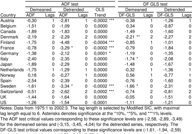
We start with PPP testing for the RER based on export unit values. The results of the ADF unit root tests are presented in Table 1. The unit root null hypothesis cannot be rejected in all but two countries: France and Sweden. When we allow for a trend, unit root is rejected only for Switzerland. A simple OLS regression on a constant and a trend indicates the presence of a trend for Canada, Spain and Switzerland. Hence, the results of both detrended ADF and simple OLS indicate that, for Switzerland, the RER based on export unit values has a deterministic trend, although the trend component amounts to only 0.04% per quarter. Nonetheless, we could not reject random walk for this series in the estimation without trend, that is, in the “demeaned” result. As Taylor (2002) puts it, “it is necessary to allow for slowly-evolving deterministic trends. As an empirical matter, they are usually found to be “small”. However, their omission would undoubtedly upset any study of the deviations of real exchange rates over the very long run”.
test, the DF-GLS test rejects the unit root null for Sweden. Nevertheless, with the DF-GLS test there are four countries, instead of only two, for which the unit root can be rejected: France, Germany, Italy and the Netherlands. The detrended Switzerland RER series also does not present a unit root, and so does the detrended France series. Comparing the two tests, the DF-GLS captures convergence in a larger number of countries compared to the ADF test, as expected. Yet, we could not reject the present of unit roots in most of the series, in both tests.
Even though the export unit values index only includes tradable goods, the PPP hypoth-esis is valid for only, at most, four countries out of sixteen. The reason for this result may be that the basket of goods composition di¤ers substantially across countries. When comparing export unit values for two countries, we are comparing the weighted values for two di¤erent basket of goods. Hence, even if the traded goods prices are arbitraged by trade, the value of the index could follow di¤erent paths in di¤erent countries due to the di¤erence in the index composition in each of the countries.
For the RER series based on wholesale price indices, the ADF tests does not reject the unit root null for any of the series, as shown in Table 2. In the same table, using the more powerful DF-GLS, unit root is rejected for six countries: Finland, France, Germany, Italy, Switzerland and Spain. For the detrended estimation, unit root is not rejected for any of the countries. As we will see, this is the RER series for which PPP is valid for a larger set of countries.
Table 3 presents the results of the ADF and DF-GLS tests for the RER series constructed as CPI ratios. The presence of unit root cannot be rejected for any of the countries, using the ADF test. Using the DF-GLS test in four countries: Denmark, Finland, Italy and Norway, the results do not present unit root in their RER series. The result for Switzerland RER series is analogous to the one for its RER series based on export unit values: we cannot reject the unit root null for its demeaned series, but, once a trend is included, the series becomes stationary. This result indicates that there is a also deterministic trend in the RER based in CPI ratios, and this is the reason for the non validity of PPP hypothesis.
odd cases are Denmark and Norway, for their RER series present unit roots when based on WPIs, but not when using CPIs.
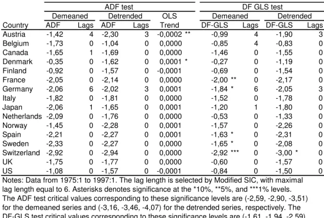
The results of PPP testing for RER based on unit labor cost and on normalized unit labor cost are very similar. The ADF test does not detect stationarity for any of the two series, as shown in Tables 4 and 5. Adding a trend to the estimation results in rejection of unit root for France for the two series, and for Sweden for the unit labor cost series. The estimation with DF-GLS somewhat improves the results. Table 4 shows that the unit root null is rejected for Denmark, Italy and Sweden, for the RER based on unit labor cost. For the normalized series, unit root is rejected only for Canada and Denmark, as presented in Table 5. We cannot reject unit roots for any of the detrended estimation, for the two sets of RER series. This means that no deterministic trend explain the unit root evidence.
These results indicate that the RER proxied by the ratio of unit labor cost, normalized or not, is a poor proxy for the relative prices of tradable goods. One possible explanation is the fact that the capital to labor ratio di¤ers substantially across countries, so that the labor cost becomes a poor re‡ection of relative prices.
The results for the value-added-RER series are interesting. The results from ADF, in Table 6, detects no unit root. The DF-GLS, on the other hand, rejects the unit root null for …ve countries: France, Germany, Spain, Sweden and Switzerland. These results, in Table 6, are close to the ones for the RER series based on WPI, for which stationarity was found for six countries.
The worst results are those for the RER measured as a ratio of foreign countries CPI and domestic country WPI. No evidence of stationarity of theses series were found, using both the ADF and the DF-GLS unit root tests. The results are presented in Table 7. This proxy for RER su¤ers from two of the problems that could causes PPP deviations, as detected in equation (2.4): some of the price indices have a large share of nontradable goods (the CPIs), and the composition of foreign and domestic indices are substantially di¤erent (as evinced in simultaneously CPIs and WPIs). Therefore the results suggest that the long run RER may be a function of real variables when the price indices do not measure the same basket of goods in all countries and the goods are not tradables.
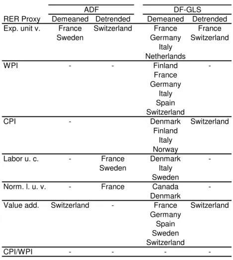
that it is more competent to reject the unit root null when the speed of convergence is low. The RER proxy leader in stationarity is the one constructed with WPIs ratios, presenting PPP evidence for six of the sixteen countries studied when we use DF-GLS test with de-meaned series. This is a signal that this price index is the one that best …ts the requirement for PPP: more uniform goods composition across countries and low share of nontradable goods. The second place goes to the RER based on value added. PPP evidence was found for …ve of the countries, for this RER proxy. The third position is a draw between the RER based on export unit values and the one based on CPIs ratio: they both yield PPP for four of the countries studied. Unquestionably, the very last place goes to the RER constucted as the ratio between foreign countries CPIs and domestic country WPI.
Looking at the countries’ perspective, France is the country for which PPP evidence was found in the larger number of RER series. There is some evidence of PPP for France for …ve of the seven RER proxies used. Switzerland and Italy follow closely, with PPP evidence for four of the RER series. No evidence of PPP was found in any of the series for …ve countries: Austria, Belgium, Japan, United Kingdom and United States.
2.6
Concluding Remarks
There is an extensive literature testing the PPP hypothesis, most of it using either CPIs or WPIs ratios as proxies of relative currencies purchasing power, that is, of the RER. Looking closely at the PPP argument, it states that the currencies purchasing power should not change when comparing the same basket of goods across countries, and these goods should all be tradable. Neither of those price indices used in PPP testing fully satisfy these two criteria: they include nontradable goods and their basket composition di¤ers across countries. We observe that, if PPP is valid at all, it should be captured by the relative price indices that best …ts these two features. Hence, we ran a horse race among six di¤erent price indices available from the IMF database to see which one would yield higher PPP evidence. We used RER proxies measured as the ratio of export unit values, wholesale prices, value added de‡ators, unit labor costs, normalized unit labor costs and consumer prices. PPP was tested using both the ADF and the DF-GLS unit root test of the RER series.
series. This is an indication that, from all indices used, WPI seems to be the one with larger composition of tradable goods and with one least variation in its basket of goods composition across countries.
The second best RER measure was the value added de‡ators. On the one hand, this is an index that includes the cost of all factors of production. On the other hand, the index composition may vary substantially across countries due to the lack of cross-country comparability.
Unit labor costs and normalized unit labor cost proved to be poor measures of tradable goods, as PPP evidence was found for a small number of countries, when RER was measured by them. However, the worst measure of all was the RER based on the ratio of foreign CPI and domestic WPI. No evidence of PPP at all was found for this measure meaning that the fundamentals could be a¤ecting the long run RER.
Finally, deterministic trends were found to be signi…cant in several cases, possibly indi-cating some Balassa-Samuelson e¤ect.
Bibliography
[1] Balassa, Bela, 1964, “The Purchasing Power Parity Doctrine: A Reappraisal,” Journal of Political Economy 72: 584-96.
[2] Cassel, Gustav, 1918, “Abnormal Deviations in International Exchanges,” The Eco-nomic Journal 28 (112): 413-415.
[3] Cheung, Yin-Wong and Kon S. Lai, 1998, “Parity Reversion in Real Exchange Rates during the Post-Bretton Woods Period,” Journal of International Money and Finance
17(4): 597-614.
[4] Cheung, Yin-Wong and Kon S. Lai, 1993, “Long-run purchasing poer parity during the recent ‡oat,” Journal of International Economics 34: 181-192 (North-Holland).
[5] Chinn, Menzie, 1998, “Before the Fall: Were East Asian Currencies Overvalued”,
Emerging Markets Review 1 (2).
[6] De Gregorio, José, Alberto Giovannini and Holger C. Wolf, 1994, “International Evi-dence on Tradables and Nontradables In‡ation,” European Economic Review 38(June). [7] Dornbusch, Rudiger, 1987, “Purchasing Power Parity,” in John Eatwell, Murray Milgate and Peter Newman (eds.) The New Palgrave: A Dictionary of Economics, vol. 3: 1075-85 (New York: Stockton Press, 3rd ed.).
[8] Edwards, Sebastian, 1989, Real Exchange Rates, Devaluation and Adjustment: Ex-change Rate Policy in Developing Countries (Cambridge, Massachusetts: MIT Press). [9] Edwards, Sebastian, 1994, “Real and Monetary Determinants of Real Exchange Rate
Estimating Equilibrium Exchange Rates (Washington: Institute for International Eco-nomics).
[10] Elbadawi, Ibrahim, 1994, “Estimating Long-Run Equilibrium Real Exchange Rates,” in John Williamson (ed.) Estimating Equilibrium Exchange Rates (Washington: Institute for International Economics).
[11] Elliott, Graham, Thomas J. Rothenberg and James H. Stock, 1996, “E¢cient Tests for an Autoregressive Unit Root,” Econometrica 64(4): 813-36.
[12] Engel, Charles, 1999, “Accounting for US Real Exchange Rate Changes,” The Journal of Political Economy 107 (3): 507-538.
[13] Frenkel, Jacob A., 1978, “Purchasing Power Parity: Doctrinal Perspective and evidence from 1920s”, Journal of International Economics 8: 169-91.
[14] Froot, Kenneth A. and Kenneth Rogo¤, 1995, “Perspectives on PPP and Long Run Real Exchange Rates,” in Gene M. Grossman and Kenneth Rogo¤ (eds.) Handbook of International Economics, vol. 3 (Amsterdam: North-Holland).
[15] International Monetary Fund, 1984, “Issues in the Assessment of the Exchange Rates of Industrial Countries”, IMF Occasional Paper No. 29.
[16] Ito, Takatoshi, Peter Isard, Steven Symansky and Tamim Bayoumi, 1996, “Exchange Rate Movements and Their Impact in Trade and Investment in the APEC Region”, IMF Occasional Paper No. 145.
[17] Keynes, John M., 1932, Essays in Persuasion (New York: Hartcourt Brace).
[18] Rogo¤, Kenneth, 1996, “The Purchasing Power Parity Puzzle,” Journal of Economic Literature 34: 647-68.
[19] Samuelson, Paul A., 1964, “Theoretical Notes on Trade Problems”,Review of Economics and Statistics 46: 145-54.
[21] Taylor, Alan N., 2002, “A Century of Purchasing-Power Parity,” Review of Economics and Statistics 84(1): 139-50.
2.7
Appendix
This appendix presents the methodologies for the computation of weights (Wij) that is
published in the Fund’s International Financial Statistics.
We begin with the methodology for the weights used in the computation of RER based on relative export unit values, wholesale prices, value added de‡ators, unit labor costs and normalized unit labor costs.
From January 1991 onwards, Wij uses data on trade and consumption of manufactured
goods over the period 1989-91. Before that, the weights used in the computation of MRER were based on 1980 data.
Let there bek markets in which the producers of countryi and country j compete. Let Tlk represent the sales of countrylin market k:Letskj be countryj0s market share in market k and wki be the share of countryi0s output sold in market k;which is to say:
skj = T
k j P
l
Tlk and (2.9)
wik = T
k i P
n
Tin: (2.10)
Then, the weight attached to country j by country iis:
Wij = P
k
wk iskj P
k
wk
i(1 ski)
: (2.11)
The world is divided into 22 markets, the …rst 21 markets being the countries2 for which
MRER were being computed by IMF and the last market is called ”Rest-of-the-World”. Next we will present the second methodology that describes the weights used in the computation of MRER based on consumer price index.
From January 1990 onwards, Wij is weighted by a set of weights based on trade in
manufactures, non-oil primary commodities and, for a set of 46 countries and regions3 in
which services accounted to meet more than 20 percent of all exports in 1989-90, tourism services covering the three-year period 1988-1990. Prior to January 1990, the weights used are those of the three-year span 1980-82.
Those weights were then aggregated to arrive at the overall weight attributed to country i to country j, Wij:Speci…cally:
Wij = i(M)Wij(M) + i(P)Wij(P) + i(T)Wij(T); (2.12)
where Wij(M); Wij(P) and Wij(T) are weights based on trade in manufactures, primary
commodities and tourism services. The factors i(M); i(P) and i(T) are the shares of
trade in manufactures, primary commodities and tourism services in country i0s external trade, with external computed as the sum of trade in manufactures, primary commodities and tourism services. Observe that i(T) = 0 for a set of countries in which services
accounted to meet less than 20 percent of all exports for 1989-90. For these countries, i(M)
and i(P) are the shares of trade in manufactures and primary commodities in total trade,
with total trade being computed as the sum of trade in these two categories.
The weights based on trade in manufactures,Wij(M); and on trade in tourism, Wij(T);
were computed in a manner analogous to equation (2.11). These weights are a weighted sum of a weight re‡ecting competition in the domestic market, a weight re‡ecting competi-tion abroad against domestic producers and a weight re‡ecting competicompeti-tion abroad against
2These 21 countries are Australia, Austria, Belgium, Canada, denmark, Finland, France, Germany,
Greece, Ireland, Italy, Japan, the Netherlands, New Zealand, Norway, Portugal, Spain, Sweden, Switzer-land, the United Kingdom and the United States.
3These 46 countries and regions are Antigua and Borbuda, Austria, The Bahamas, Barbados, Belize,
exporters.
The weights based on trade in primary commodities, Wij(P); were computed in a very
di¤erent way. Contrary to manufactured goods and tourism services, primary commodities are assumed to be homogeneous goods. Then, for each commodity, the weight attached to country j by any country should re‡ect the importance of country j as either a seller or a buyer in the world market. Therefore, for country i; the weight attached to country j; Wij(P); should be a (normalized) sum over all commodity markets of the product of the
OLS
Country ADF Lags ADF Lags Trend DF-GLS Lags DF-GLS Lags Austria -2,12 4 -2,11 4 0,0000 -0,34 4 -1,44 4 Belgium -2,55 0 -2,20 0 0,0000 -0,94 0 -1,58 0 Canada -0,31 0 -2,40 0 -0,0002 ** 1,53 0 -2,46 0 Denmark -1,20 0 -1,52 0 0,0000 -1,22 0 -1,32 0 Finland -2,19 0 -2,14 0 0,0000 -0,68 0 -1,74 0 France -2,61 * 0 -2,90 0 0,0000 -2,60 *** 0 -2,87 * 0 Germany -1,77 0 -1,93 0 0,0000 -1,75 * 0 -2,02 0 Italy -2,41 0 -2,43 0 0,0000 -2,36 ** 0 -2,46 0 Japan -1,21 0 -1,74 0 0,0001 -1,21 0 -1,48 0 Netherlands -2,42 0 -2,54 0 0,0000 -2,04 ** 0 -2,23 0 Norway -2,49 1 -2,79 1 -0,0001 -0,94 1 -2,43 1 Spain -1,30 0 -2,15 0 0,0001 * -1,25 0 -1,79 0 Sweden -2,69 * 0 -2,43 0 0,0000 -1,06 0 -1,76 0 Switzerland -1,06 0 -3,40 * 0 0,0004 *** -0,12 0 -3,32 ** 0
UK -2,13 0 -2,64 0 0,0001 -0,81 0 -2,48 0
US -1,51 0 -1,50 0 0,0000 -0,69 0 -1,19 0
Notes: Data from 1975:1 to 1998:2. The lag length is selected by Modified SIC, with maximal lag length equal to 6. Asterisks denotes significance at the *10%, **5%, and ***1% levels. The ADF test critical values corresponding to these significance levels are (-2,58, -2,89, -3,51) for the demeaned series and (-3,16, -3,46, -4,06) for the detrended series, respectively. The DF-GLS test critical values corresponding to these significance levels are (-1,61, -1,94, -2,59) for the demeaned series and (-2,77, -3,07, -3,62) for the detrended series, respectively.
Detrended DF GLS test
Demeaned Detrended Demeaned ADF test
OLS
Country ADF Lags ADF Lags Trend DF-GLS Lags DF-GLS Lags Austria -1,58 2 -2,63 2 -0,0001 ** -1,51 2 -2,37 2 Belgium -1,38 1 -1,10 0 0,0000 -0,02 1 -1,08 0 Canada -1,88 0 -1,77 0 0,0000 -1,04 0 -1,56 0 Denmark -1,51 0 -1,83 0 0,0000 -1,52 0 -1,65 0 Finland -1,30 0 -1,46 0 0,0000 -1,71 * 1 -1,50 0 France -1,83 0 -1,92 0 0,0000 -1,74 * 0 -1,80 0 Germany -1,69 0 -2,08 0 0,0000 -1,69 * 0 -1,86 0 Italy -1,90 0 -1,92 0 0,0000 -1,89 * 0 -1,95 0 Japan -1,57 0 -1,71 0 0,0001 -1,59 1 -1,86 0 Netherlands -1,39 0 -1,54 0 0,0000 -1,39 0 -1,45 0 Norway -1,51 0 -0,58 0 0,0000 -0,52 0 -0,92 0 Spain -2,21 0 -2,16 0 0,0000 -2,21 ** 0 -2,22 0 Sweden -2,30 0 -2,23 0 0,0000 -1,52 0 -2,03 0 Switzerland -2,47 0 -2,70 0 0,0001 -2,49 ** 0 -2,65 0
UK -1,77 0 -2,22 0 0,0001 -0,50 0 -2,09 0
US -1,12 0 -1,57 0 -0,0001 -1,22 0 -1,40 0 Notes: Data from 1975:1 to 1997:1. The lag length is selected by Modified SIC, with maximal lag length equal to 6. Asterisks denotes significance at the *10%, **5%, and ***1% levels. The ADF test critical values corresponding to these significance levels are (-2,58, -2,90, -3,51) for the demeaned series and (-3,16, -3,46, -4,07) for the detrended series, respectively. The DF-GLS test critical values corresponding to these significance levels are (-1,61, -1,94, -2,59) for the demeaned series and (-2,78, -3,07, -3,63) for the detrended series, respectively.
ADF test DF GLS test
Demeaned Detrended Demeaned Detrended
OLS
Country ADF Lags ADF Lags Trend DF-GLS Lags DF-GLS Lags Austria -1,52 0 -1,59 0 0,0000 -0,74 0 -1,66 0 Belgium -1,63 1 -1,76 1 0,0000 -0,90 1 -1,75 1 Canada -1,13 1 -1,58 0 -0,0001 -0,20 1 -1,59 0 Denmark -1,85 0 -2,13 0 0,0000 -1,81 * 0 -1,90 0 Finland -1,64 1 -1,55 0 0,0000 -1,64 * 1 -1,37 0 France -1,63 0 -2,26 0 0,0000 -0,61 0 -2,25 0 Germany -2,00 0 -1,94 0 0,0000 -0,81 1 -1,54 0 Italy -2,00 1 -1,47 0 0,0000 -1,98 ** 1 -2,07 1 Japan -2,08 1 -1,79 0 0,0001 -0,71 1 -1,72 0 Netherlands -1,76 0 -1,73 0 0,0000 -1,16 0 -1,82 0 Norway -1,97 0 -1,65 0 0,0000 -1,64 * 0 -1,93 0 Spain -1,84 0 -1,73 0 0,0000 -1,22 0 -1,62 0 Sweden -1,10 0 -2,12 0 -0,0001 * 0,01 0 -2,16 0 Switzerland -2,12 0 -2,89 0 0,0001 * -1,45 0 -2,91 * 0
UK -1,69 0 -1,95 0 0,0001 -1,09 0 -1,97 0
US -1,04 0 -1,08 0 0,0000 -0,92 0 -1,16 0
Notes: Data from 1975:1 to 2002:3. The lag length is selected by Modified SIC, with maximal lag length equal to 6. Asterisks denotes significance at the *10%, **5%, and ***1% levels. The ADF test critical values corresponding to these significance levels are (-2,58, -2,89, -3,49) for the demeaned series and (-3,15, -3,45, -4,04) for the detrended series, respectively. The DF-GLS test critical values corresponding to these significance levels are (-1,61, -1,94, -2,59) for the demeaned series and (-2,73, -3,02, -3,57) for the detrended series, respectively.
ADF test DF GLS test
Demeaned Detrended Demeaned Detrended
OLS
Country ADF Lags ADF Lags Trend DF-GLS Lags DF-GLS Lags Austria -0,30 1 -2,81 1 -0,0002 *** -0,38 1 -1,26 1 Belgium -1,51 0 -1,09 0 0,0000 0,34 0 -0,87 0 Canada -1,89 0 -1,83 0 0,0000 -1,49 0 -1,60 0 Denmark -2,19 2 -2,29 2 0,0000 -2,21 ** 2 -2,27 2 Finland -1,75 0 -4,48 0 -0,0004 *** -0,85 1 -1,01 0 France -0,78 0 -3,29 * 0 -0,0002 *** -0,79 0 -1,84 0 Germany -1,38 0 -2,12 0 0,0001 * -1,19 0 -1,35 0 Italy -2,40 0 -2,35 0 0,0000 -1,74 * 0 -2,08 0 Japan -1,89 0 -2,29 0 0,0000 -1,48 0 -1,67 0 Netherlands -1,75 1 -1,29 1 0,0000 -0,32 1 -1,36 1 Norway 0,18 0 -0,27 1 0,0000 0,56 1 -0,77 1 Spain -2,54 0 -2,39 0 0,0000 -0,76 0 -1,60 0 Sweden -1,61 0 -3,34 * 0 -0,0002 *** -1,66 * 0 -2,31 0 Switzerland -0,51 2 -2,62 2 0,0002 *** -0,74 2 -0,81 2
UK -1,44 0 -1,64 0 0,0000 -0,05 0 -1,51 0
US -1,26 0 -1,54 0 -0,0001 -1,11 0 -1,21 0 Notes: Data from 1975:1 to 2002:3. The lag length is selected by Modified SIC, with maximal lag length equal to 6. Asterisks denotes significance at the *10%, **5%, and ***1% levels. The ADF test critical values corresponding to these significance levels are (-2,58, -2,89, -3,49) for the demeaned series and (-3,15, -3,45, -4,04) for the detrended series, respectively. The DF-GLS test critical values corresponding to these significance levels are (-1,61, -1,94, -2,59) for the demeaned series and (-2,73, -3,02, -3,57) for the detrended series, respectively.
ADF test DF GLS test
Demeaned Detrended Demeaned Detrended
OLS
Country ADF Lags ADF Lags Trend DF-GLS Lags DF-GLS Lags Austria -0,55 0 -2,79 1 -0,0002 *** -0,53 0 -1,38 1 Belgium -2,10 0 -1,37 0 0,0000 0,71 1 -0,87 0 Canada -2,00 1 -2,07 1 0,0000 -1,80 * 1 -1,90 1 Denmark -2,34 0 -2,56 0 0,0000 -2,32 * 0 -2,41 0 Finland -1,30 0 -4,09 0 -0,0004 *** -0,83 0 -0,98 0 France -0,38 0 -3,44 * 0 -0,0002 *** -0,42 0 -1,55 0 Germany -1,22 0 -2,14 0 0,0001 * -1,14 0 -1,32 0 Italy -2,45 0 -2,39 0 0,0000 -1,56 0 -1,96 0 Japan -1,91 0 -2,39 0 0,0001 -1,50 0 -1,70 0 Netherlands -1,75 0 -1,20 0 0,0000 0,07 0 -1,21 0 Norway -1,15 1 0,01 0 0,0001 1,30 1 -0,38 0 Spain -2,48 0 -2,44 0 0,0000 -0,83 0 -1,91 0 Sweden -1,15 0 -3,01 0 -0,0002 *** -1,56 0 -2,40 0 Switzerland -0,43 2 -2,51 2 0,0002 *** -0,68 2 -0,88 2
UK -1,18 0 -1,64 0 0,0000 0,07 0 -1,61 0
US -1,25 0 -1,57 0 -0,0001 -1,02 0 -1,15 0 Notes: Data from 1975:1 to 2002:3. The lag length is selected by Modified SIC, with maximal lag length equal to 6. Asterisks denotes significance at the *10%, **5%, and ***1% levels. The ADF test critical values corresponding to these significance levels are (-2,58, -2,89, -3,49) for the demeaned series and (-3,15, -3,45, -4,04) for the detrended series, respectively. The DF-GLS test critical values corresponding to these significance levels are (-1,61, -1,94, -2,59) for the demeaned series and (-2,73, -3,02, -3,57) for the detrended series, respectively.
ADF test DF GLS test
Demeaned Detrended Demeaned Detrended
OLS
Country ADF Lags ADF Lags Trend DF-GLS Lags DF-GLS Lags Austria -1,42 4 -2,30 3 -0,0002 ** -0,99 4 -1,90 3 Belgium -1,73 0 -1,04 0 0,0000 -0,85 4 -0,83 0 Canada -1,65 1 -1,69 0 0,0000 -1,46 0 -1,55 0 Denmark -0,35 0 -1,62 0 0,0001 * -0,27 0 -1,19 0 Finland -0,92 0 -1,57 0 -0,0001 -0,69 0 -1,54 0 France -2,05 0 -2,14 0 0,0000 -2,00 ** 0 -2,17 0 Germany -2,06 6 -2,02 3 0,0001 -1,84 * 6 -2,05 3 Italy -1,82 0 -1,81 0 0,0000 -1,52 0 -1,78 0 Japan -2,06 1 -1,65 0 0,0001 -1,20 1 -1,80 0 Netherlands -2,09 0 -1,76 0 0,0000 -0,53 0 -1,33 0 Norway -1,45 0 -2,28 0 0,0001 -1,57 0 -2,26 0 Spain -2,21 0 -2,27 0 0,0001 -1,63 * 0 -2,31 0 Sweden -2,33 0 -2,27 0 0,0000 -1,65 * 0 -2,08 0 Switzerland -2,92 0 -2,94 0 0,0000 -2,92 *** 0 -3,00 * 0
UK -1,75 0 -1,77 0 0,0000 -0,60 0 -1,57 0
US -1,08 0 -1,57 0 -0,0001 -0,84 0 -1,50 0 Notes: Data from 1975:1 to 1997:1. The lag length is selected by Modified SIC, with maximal lag length equal to 6. Asterisks denotes significance at the *10%, **5%, and ***1% levels. The ADF test critical values corresponding to these significance levels are (-2,59, -2,90, -3,51) for the demeaned series and (-3,16, -3,46, -4,07) for the detrended series, respectively. The DF-GLS test critical values corresponding to these significance levels are (-1,61, -1,94, -2,59) for the demeaned series and (-2,79, -3,08, -3,64) for the detrended series, respectively.
ADF test DF GLS test
Demeaned Detrended Demeaned Detrended
OLS
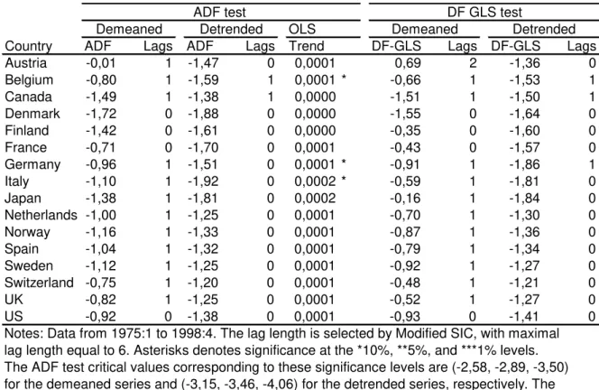
Country ADF Lags ADF Lags Trend DF-GLS Lags DF-GLS Lags Austria -0,01 1 -1,47 0 0,0001 0,69 2 -1,36 0 Belgium -0,80 1 -1,59 1 0,0001 * -0,66 1 -1,53 1 Canada -1,49 1 -1,38 1 0,0000 -1,51 1 -1,50 1 Denmark -1,72 0 -1,88 0 0,0000 -1,55 0 -1,64 0 Finland -1,42 0 -1,61 0 0,0000 -0,35 0 -1,60 0 France -0,71 0 -1,70 0 0,0001 -0,43 0 -1,57 0 Germany -0,96 1 -1,51 0 0,0001 * -0,91 1 -1,86 1 Italy -1,10 1 -1,92 0 0,0002 * -0,59 1 -1,81 0 Japan -1,38 1 -1,81 0 0,0002 -0,16 1 -1,84 0 Netherlands -1,00 1 -1,25 0 0,0001 -0,70 1 -1,30 0 Norway -1,16 1 -1,33 0 0,0001 -0,87 1 -1,36 0 Spain -1,04 1 -1,32 0 0,0001 -0,79 1 -1,34 0 Sweden -1,12 1 -1,25 0 0,0001 -0,92 1 -1,27 0 Switzerland -0,75 1 -1,20 0 0,0001 -0,48 1 -1,21 0
UK -0,82 1 -1,25 0 0,0001 -0,52 1 -1,27 0
US -0,92 0 -1,38 0 0,0001 -0,93 0 -1,41 0
Notes: Data from 1975:1 to 1998:4. The lag length is selected by Modified SIC, with maximal lag length equal to 6. Asterisks denotes significance at the *10%, **5%, and ***1% levels. The ADF test critical values corresponding to these significance levels are (-2,58, -2,89, -3,50) for the demeaned series and (-3,15, -3,46, -4,06) for the detrended series, respectively. The DF-GLS test critical values corresponding to these significance levels are (-1,61, -1,94, -2,59) for the demeaned series and (-2,79, -3,08, -3,64) for the detrended series, respectively.
ADF test DF GLS test
Demeaned Detrended Demeaned Detrended
RER Proxy Demeaned Detrended Demeaned Detrended Exp. unit v. France Switzerland France France
Sweden Germany Switzerland Italy
Netherlands
WPI - - Finland
-France Germany
Italy Spain Switzerland
CPI - Denmark Switzerland
Finland Italy Norway
Labor u. c. - France Denmark -Sweden Italy
Sweden
Norm. l. u. v. - France Canada -Denmark
Value add. Switzerland - France Switzerland Germany
Spain Sweden Switzerland
CPI/WPI - - -
-ADF DF-GLS
Chapter 3
The Relative-factor-endowment as
one of the Determinants of the Real
Exchange Rate
3.1
Introduction
There is a vast theoretical literature on the behavior of the real exchange rate (RER), de…ned as price of tradable over nontradable goods. These studies are mainly based on the inter-national trade theory that link the equilibrium RER to changes in fundamentals (see, for example Edwards, 1989 and 1994) or based on macroeconomic balance approach that makes quantitative appraisals of exchanges rates that are compatible with adequate current account positions in economies operating at potential output (see, for example Isard, Faruqee, Kin-caid and Fetherston, 2001). Our contribution is to show that the relative-factor-endowment may be also one of the determinants of the RER. According to the traditional trade theory including the nontradable good, we show theoretically that the RER is a function of relative factor prices for countries in the same cone of diversi…cation1. Thus, if the factor price
equal-ization is valid within cones, the RER should be the same for countries in the same cone of
1Countries with endowments in the same cone of diversi…cation produce the same goods with the same
diversi…cation. We also show empirically that the RER is positively correlated among coun-tries in the same cone of diversi…cation and negatively correlated among councoun-tries within di¤erent cones. The empirical result corroborates with our theoretical model.
In testing the impact of endowments on RER, this paper is most closely related to work by Bhagwati (1984). His model with two traded goods, one nontraded service, identical pro-duction functions and two factors of propro-duction: capital and labor in each sector formulates an explanation for the cheaper relative price of services in the poor countries. Bhagwati introduces the relative factor endowment argument to explain this relative price, that is the RER, based on a model where the rich and the poor countries are distributed across two cones of diversi…cation. Guerguil and Kaufman (1998) state out that the Balassa-Samuelson e¤ect and the relative factor endowment are the determinants of the RER by the supply side. Based on Bhagwati’s model, Guerguil and Kaufman state that “Relatively labor-abundant countries will exhibit lower relative wages and lower relative nontradable prices. It should be pointed out, though, that capital accumulation will not be translated into continuously higher wages, but will result instead in discrete changes when the country enters a new di-versi…cation cone. Hence, the RER will depend upon the relative factor endowment and the path of capital accumulation, but with step instead of cotinuous adjustments".
Introducing the nontradable sector in the traditional trade theory, we propose a model where each country produces two tradable goods and one nontradable good and there are two factors of production (capital and labor). We assumed that countries with endowments in the same cone of diversi…cation produce tradable goods where prices are determined externally. By the condition of pro…t maximization, the price of tradable goods determines the factor prices, which in turn, determine the price of nontradable goods. Whether the factor price equalization is valid within diversi…cation cone, the RER should be the same for countries with endowments in the same cone of diversi…cation. This is not necessarily true for countries in di¤erent diversi…cation cones.
To test our theory, we use the results of Schott (2003). He tests whether a sample of developing and developed countries are distributed across more than one cone of diversi…-cation and concludes that is distributed across two cones of diversi…diversi…-cation. Schott proposes a new methodology for testing the Heckscher-Ohlin model that permits that countries with su¢ciently disparate relative-factor-endowment to produce a di¤erent subset of goods.
and bilateral real exchange rates using monthly data from 1985 to 1995. Thereafter, we calculated two measures of correlation: Pearson Product-Moment Correlation and Spearman Rank Correlation. According to our results, the series of RER among countries in the same cone of diversi…cation (cone intensive in capital and cone intensive in labor) are positively correlated, whereas the series of RER among countries in di¤erent cones of diversi…cation is negatively correlated. Hence, the results are in conformity with our prediction.
To corroborate our …ndings, we did the Purchasing Power Parity (PPP) testing for bilat-eral real exchange rates (RER) for all countries in the sample. The results indicate that the validity of PPP hypothesis is larger among countries in the same cone of diversi…cation than among countries of di¤erent cones of diversi…cation. Therefore, the results are in conformity with our prediction.
The paper is organized as follows. Section 2 introduces the nontradable sector in the traditional trade theory and shows that the real exchange rate is a function of relative price factors. Section 3 presents the Schott’s model. Section 4 decribes the data. Section 5 analyzes the empirical results. Finally, section 6 concludes.
3.2
The Real Exchange Rate and the Relative Price
Factors
To study the possibility of RER parity among countries with endowments in the same cone of diversi…cation, we use the traditional trade theory including the nontradable good2. In our
model, there are three tradable goods, one nontradable good and two factors of production: capital and labor.
In spite of the fact that empirical research has demonstrated the importance of other factors of production beyond capital and labor as part of the countries’ production patterns (Learmer, 1984), we consider only two factors of production because, …rst, we use the em-pirical results of Schott (2003) that has built a model based on two factors of production, second, constant returns of scale and the equality of the number of goods and factors of production are essential in estabilishing a one-to-one relationship between factor prices and prices of goods.
Our model is designed with perfect factor mobility across industries within a country
and immobility across countries, small and open countries, perfectly competitive markets, identical homothetic tastes and technologies with constant returns to scale across countries. Suppose that the production functions for tradable goods are identical for all countries as follows:
Yi = minf iLi; iKig; i= 1;2;3 (3.1)
where Y denotes output,L labor input,K capital input anditradable goods for i= 1; 2or
3: Assume that tradable goods 1;2and 3 have the factor intensity as follows:
3 3
> 2
2
> 1
1
: (3.2)
From the hypothesis of our model with more goods than factors and the pro…t maxi-mization, we have three equations for two unknows (L and K) that makes the production indetermined. The literature gives us some solutions for the indeterminancy of production. Bhagwati (1972) suggests that, when the factor prices are di¤erent across countries, a coun-try’s exports must be more intensive in the factor of production that the country is abundant, than all of its imports. Bhagwati also emphazised that including transport costs on every commodity, the commodity prices would be di¤erent in trade, the factor prices would not be equalized via commodity price equalization and the indeterminancy of production would be solved. Deardor¤ (1979), in turn, agrees with Bhagwati when the trade includes only …nal goods with free trade. However, introducing intermediate goods and trade impediments, the statement of Bhagwati does not hold. To solve the indeterminancy of production, Deardor¤ (1979) suggests to consider that the countries’ endowments are so di¤erent, that they move outside of the fator price equalization set. Dornbusch, Fischer and Samuelson (1980) prove Deardor¤’s statement for a continuum of goods.
Based on Deardor¤ (1979), we show that in our model, with three tradable goods, just two tradable goods are produced in each country.
fell short of its unit cost. If a unit-value isoquant were situated inside the isocost line of one of the countries, the goods would not be produced in that country because it would make a positive pro…t. Assuming that preference for both countries were such that the demand for each tradable goods were positive, the tradable goods3, the most intensive in capital, could only be produced and exported by country A, the tradable goods 1, the most intensive in labor, could only be produced and exported by country B, and the tradable goods 2 could be produced in both countries. Therefore, each country produces two tradable goods more intensive in the factor of production which the country is abundant. Countries abundant in capital produce tradable goods 3 and 2: Countries abundant in labor produce tradable goods 1 and 2:
The general equilibrium model implies that countries with endowments (capital and la-bor) in the same cone of diversi…cation produce goods with the same factor prices. Countries with endowments in di¤erent cones use di¤erent techniques and have di¤erent factor prices. Countries with endowments in neither cones specialize in the production of one goods.
The …rst equilibrium condition in the tradable market is the pro…t maximization. Under perfect competition prices in the market of tradable goods, we have:
Pi =
w
i
+ r
i
; i= 1;2 or3 (3.3)
where Pi is the price of tradable good i; determined externally in the market of tradable
goods, w is the return on labor and r is the return on capital. Countries with endowments in the cone of diversi…cation I produce tradable goods 1 and 2 which prices are:
P1 =
w
1
+ r
1
(3.4)
P2 =
w
2
+ r
2
that, in turn, determine the factor prices wI and rI that are:
wI =
1 2 P12
P1 2 1 1 2 2
rI =
P1 1 P2 2
1 1
Analoguously, countries with endowments in the cone of diversi…cation II produce the tradable goods 2 and 3 which prices are:
P2 =
w
2
+ r
2
(3.5)
P3 =
w
3
+ r
3
that, in turn, determine the factor prices wII and rII that are:
wII =
3 2 P23
P3 2 3
3 2 2
rII =
P3 3 P2 2
3 3
2 2
:
Suppose that the production functions for nontradable goods are identical for all countries as follows:
YN =A(KN)a(LN)1 a; (3.6)
whereAis the nontradable goods productivity and the subscriptN;nontradable goods. The nontradable goods is produced by the two groups of countries with the same technology but with di¤erent techniques. From the pro…t maximization, the price of nontradable goods,PN,
may be written as follows:
PNh =Brhaw1h a h=I; II (3.7)
where B = A1 1aa a 11a and the subscript h, cone of diversi…cation. Substituting the factor prices in equation (3.7), we have the price of nontradable goods for each cone of diversi…cation.
In addition, we know that in equilibrium the demand of nontradable goods, DN, are
equal to the supply of nontradable goods, YN, for each cone of diversi…cation as follows:
We assume that the demand for nontradables in coneI is not so great as to leave enough labor and capital for the production of tradable goods 1and 2and the demand for nontrad-ables in cone II is not so great as to leave enough labor and capital for the production of tradable goods 2 and 33.
Consider that the tradable goods price for cone of diversi…cationI; PI are geometrically
weighted averages of P1 and P2, with weights and (1 ) respectively, and the tradable goods price for cone of diversi…cationII; PII are geometrically weighted averages ofP
2 and
P3, with weights and (1 ) respectively, as follows:
PI = P1+ (1 )P2 (3.9)
PII = P2+ (1 )P3: (3.10)
The RER for countries in the cone of diversi…cationI may be written as:
RERIT =N = P
I
PNI =
wI
rI 1 +
(1 )
2 + 1 +
(1 ) 2 wI rI 1 a B
=f wI rI
(3.11)
and the RER for countries in the cone of diversi…cation II may be written as:
RERIIT =N = P
II
PII N
=
wII
rII 2 +
(1 )
3 + 2 +
(1 ) 3 wII rII 1 a B
=g wII rII
: (3.12)
The equations (3.11) and (3.12) indicate that the RER is a function of relative price factors for countries in the same cone of diversi…cation. Whether the factor price equalization is valid within cones, the RER should be the same for countries with endowments in the same cone of diversi…cation.
3.3
The Model of Schott (2003)
To test the Heckscher-Ohlin (HO) model, Schott (2003) proposes an empirical methodology that allows countries to produce di¤erent subsets of goods. With two factors of production,
just tradable goods and equal number of factors and goods in each cone of diversi…cation, his model is based on the traditional trade theory.
Schott states that countries with su¢ciently di¤erent relative-factor-endowments may be distributed over more than one cone of diversi…cation. He uses the Rybzinski Theorem, which argues that at constant goods prices, an increase in the supply of one factor will increase the output of the goods which uses that factor intensively and reduces the output of the other goods, to analyze if the countries fall into more than one single cone of diversi…cation. If the sample of countries is into a single cone of diversi…cation then the Rybczynski relationship can be estimated using a cross section of countries’ output per worker and capital-labor as follows:
Qic
Lc
= 1i+ 2i
Kic
Lc
+"ic (3.13)
where c denotes the country, i denotes the industry, Q denotes the output, L denotes the total workforce and K denotes the capital.
If the countries are distributed among several cones of diversi…cation, the correct speci-…cation for each cone is the following4:
Qic Lc = T+1 X t=1 1itIt
Kc
Lc
> t + 2it
Kc
Lc
It
Kc
Lc
> t +"ic (3.14)
where t (1; T 1) means capital-labor ratio marking the borders between cones, T is the
number of knots, It n
Kc
Lc > t
o
= 1 if Kc
Lc > t and It
n Kc
Lc > t
o
= 0 if Kc
Lc 6 t, and the
capital-labor ratio of country c is de…ned as the capital per labor ratio of each industry weighted by labor as follows:
Kc
Lc
= i ILi
Ki
Li
i ILi
: (3.15)
To estimate the development path, it is necessary to de…ne what is an industry. The standard way to de…ne industry is the ISIC industry that groups output according to sim-ilarity of end use industry. The Schott’s analysis shows that this de…nition of industry is not adequate to test trade theory. His paper shows that, for 14 three-digit ISIC industries and 34 countries, the capital intensity(Kic
Lc )varies substantially by industry across countries,
which is interpreted as a signal of intra-industry product variation. The presence of within-industry heterogeneity motivates the introduction of a new methodology to group output
according to a new de…nition of industry. Schott suggests to group the output, referred to as “Heckscher-Ohlin Aggregates”, according to country-industry input intensity instead of end use. Thus, HO Aggregate n is the sum of country’s output in all ISIC aggregates with capital intensity between the maximum and minimum capital intensity for that aggregate.
With the new de…nition of industry, Schott (2003) tests if development paths based on HO Aggregates contain a kink. He tests the null hypothesis of a single-cone model (with two HO Aggregates) against alternate hypothesis of two cones of diversi…cation (with three HO Aggregates) and three cones of diversi…cation (with four HO Aggregates) based on the Bootstrap p-values. The result indicates that the sample of 45 countries, he uses developed and developing countries, are distributed across two cones of diversi…cation in 1990, each producing a subset of manufactures.
Thus, by the model presented by Schott, labor abundant countries should have endow-ments between HO aggregates labor intensity and capital abundant countries should have endowments between HO aggregates capital intensity. This result is met for the majority of 45 countries, but not for all of them. Denmark, Finland and Ireland, for example, are capi-tal abundant economies and have positive output in all HO aggregates. Another example is Turkey, that is labor abundant economy but have positive output in HO aggregates capital intensity.
In the following section, we describe the data used to build RER.