Purchasing power parity: the choice of price index

N

₅₈₈

_{ISSN 0104-8910}

Purchasing Power Parity: The Choice of Price

Index

Maria Cristina Terra, Ana Lucia Vahia de Abreu

Os artigos publicados são de inteira responsabilidade de seus autores. As opiniões

neles emitidas não exprimem, necessariamente, o ponto de vista da Fundação

Purchasing Power Parity: The Choice of Price

Index

Maria Cristina T. Terra

EPGE/FGV

Ana Lucia Vahia de Abreu

EPGE/FGV

Abstract

Looking closely at the PPP argument, it states that the currencies purchasing power should not change when comparing the same basket goods across countries, and these goods should all be tradable. Hence, if PPP is valid at all, it should be captured by the relative price indices that best …ts these two features. We ran a horse race among six di¤erent price indices available from the IMF database to see which one would yield higher PPP evidence, and, therefore, better …t the two features. We used RER proxies measured as the ratio of export unit values, wholesale prices, value added de‡ators, unit labor costs, normalized unit labor costs and consumer prices, for a sample of 16 industrial countries, with quarterly data from 1975 to 2002. PPP was tested using both the ADF and the DF-GLS unit root test of the RER series. The RER measured as WPI ratios was the one for which PPP evidence was found for the larger number of countries: six out of sixteen when we use DF-GLS test with demeaned series. The worst measure of all was the RER based on the ratio of foreign CPIs and domestic WPI. No evidence of PPP at all was found for this measure.

Keywords: real exchange rate, price indices, purchasing power parity JEL Classi…cation Number: F31, F41

1

Introduction

The purchasing power parity (PPP) hypothesis, in its original formulation,

states that the price levels of two countries should be equal, when measured

by the same currency. This is an old idea in economics, but the term was coined

only in 1918 by Gustav Cassel. As Cassel (1918) puts it, “(a)s long as anything

like free movement of merchandise and a somewhat comprehensive trade

be-tween the two countries takes place, the actual rate of exchange cannot deviate

very much from this purchasing power parity.”

Although ever since some variant of PPP has been the building the block for

modeling exchange rates long-run behavior, empirical evidence on its validity is,

at best, controversial. PPP does not seem to hold in the short run at all, which

…ts economists assessment that PPP should not hold continuously. However,

empirical evidence on long run validity of PPP is also scant. The empirical

literature on the subject has investigated possible reasons for the failure of

…nding hard evidence on long run PPP. Part of the literature credits this failure

to the combination of slow speed of convergence, high short run volatility, and

not long enough periods of time for testing the long run behavior of the series,

for the studies concentrate on post-Bretton-Woods data. The idea is that, with

a long enough time span, data on prices and exchange rates would deliver PPP.

(See Froot and Rogo¤, 1995, and Rogo¤, 1996.)

Several studies using long span data sets do …nd more consistent evidence of

long-run PPP (see Sarno and Taylor, 2002, for a brief review of this literature).

The problem with covering a long time frame is that they encompass several

di¤erent exchange rate regimes. It would be desirable to limit the sample to the

pos-Bretton-Woods period. Long time periods are also more prone to include

periods with real shock that shift the equilibrium real exchange rate (RER).

Another strand of the literature tries to circumvent the short period of time

after Bretton Woods by using panel data. Several such studies reject random

walk for the panel. These results, however, solely indicates that random walk

is rejected for at least one of the RERs used. They do not provide evidence of

PPP holding for all of them. Sarno and Taylor (2002) also discuss the results

of this literature.

ex-change rate dynamics. The idea is that transaction costs would yield deviations

from PPP, which, in turn, would follow a mean reverting nonlinear process.

This would also explain PPP deviations for long periods of time. Sarno and

Taylor (2002) present a thorough discussion of this evolving line of research.

An old concern about PPP testing, dating back to Keynes (1932), is the

very choice of the price indices to be used. The ideal index should measure

the exact same basket of goods in all countries, and these goods should all be

tradable. Such an index does not exit, though. The most commonly indices

used for testing PPP are Consumer Price Index (CPI) and Wholesale Price

Index (WPI). A positive feature of these indices is that they are readily available

for most countries and for long time frames. On the negative side, these indices

include nontradable goods and they do not measure a common basket of goods

across countries. The CPI includes a larger share of nontradable goods than the

WPI, hence, one could argue, the WPI would better suit the PPP concept.

This paper revisits this original debate over the price index choice, which

should be of an index with the most share of tradable goods and without much

variation on the composition of its goods basket across countries. Using PPP

testing as a device for spotting those two features, we perform a horse race

among six di¤erent price indices available from the International Monetary Fund

(IMF). We would expect that, if PPP is valid at all, it would be captured

when measuring prices by the price index most in line with those two features.

We perform unit root tests for multilateral real exchange rate measures for 16

industrialized countries, for the period from 1975 to 2002. The price indices

used are export unit values, wholesale prices, value added de‡ators, unit labor

costs, normalized unit labor costs and consumer prices.

There are studies that test the PPP hypothesis for di¤erent price indices

such as Dornbush (1987) that uses CPI, GDP de‡ator, the GDP de‡ator for

evi-dence of PPP for all price indices studied. Chinn (1998) also implements the

PPP testing for di¤erent price indices, for several Asian economies. He uses

CPI, WPI, PPI and export unit value index. The PPI based results indicate

some support for the PPP hypothesis.

Regarding the estimation method, the very early empirical literature tested

PPP by estimating simple ordinary least square regressions of price indices on

exchange rates. With the evolution of time series econometric modeling, unit

root tests based either on augmented Dickey-Fuller (ADF) or variance ratio tests

became popular in this literature, along with cointegration studies. Economists

have identi…ed the low power of those tests as one possible explanation for the

failure to reject random walk from RER series. Sarno and Taylor (2002) perform

a Monte Carlo experiment where they simulate data based on a AR(1) model for

the RER using di¤erent values for the autoregressive coe¢cient, as estimated

in the literature. Using the simulated data, they …nd that “the probability of

rejecting the null hypothesis of a random walk real exchange rate, when, in fact,

the real rate is mean reverting, would only be somewhere between about 5 and

7.5 percent.” To mitigate this problem, we follow Taylor (2002) and use the

Dickey-Fuller test using generalized least squares (DF-GLS) developed by Elliot

and al. (1996). This test is a modi…cation of ADF test that increases its power

without otherwise altering the method of testing.

Our main results are the following. First, the RER constructed with WPIs

supports the PPP hypothesis for the larger number of countries. Hence, this

index seems to be the one that best represents tradadable goods with similar

basket of goods for all countries. Second, when using export unit values, the

PPP is veri…ed for only 4 countries. This index includes only goods that are

actually traded by the country, hence its goods baskets composition most

prob-ably di¤ers across countries to a greater extent, compared to the other indices.

some Balassa-Samuelson e¤ect. Fourth, for the RER measured as the ratio of

foreign CPI and domestic WPI, we …nd no evidenc of PPP holding. This is

consistent with the idea that CPI has a large share of nontradable goods which

are not arbitraged across countries.

The paper is organized as follows. Section two presents the purchasing power

parity argument, and its relation to the price indices used to calculate relative

purchasing power. The methodology used in the empirical exercises is presented

in section three. Section four presents the data and section …ve the empirical

results. Finally, section 6 concludes.

2

Purchasing Power Parity

Absolute PPP states that, abstracting from any trade frictions, price levels in

two economies should be equal, when measure in the same currency, that is:

EP

P = 1; (1)

whereE is the exchange rate, andP andP are the price indices in home and foreign countries, respectively. In reality, impediments to trade, such as

trans-port costs and trade barriers, prevent prices to be perfectly equalized. Trade

restrictions do not preclude prices from being arbitraged, though, so that prices

in di¤erent countries should be closely related. Relative PPP allows for

obsta-cles to trade that drive a wedge between the purchasing power of currencies. It

states that exchange rate change should re‡ect relative prices changes:

b

E=Pb P ;c (2)

where Xb = dlog_XX: Relative PPP should hold when the di¤erence in prices driven by trade frictions do not change over time.

Going from absolute PPP to relative PPP is not only a way of getting around

problem of prices that are only reported as indices, as opposed to an actual

price of a basket of goods. As the price indices are normalized in a base year,

even if absolute PPP held, equation (1) would not hold.

PPP, in both its absolute or relative versions, depicts a relation between

tradable goods, for these are the goods that are arbitraged by international

trade. Hence, the price indices used for testing either equation (1) or equation

(2) should contain only tradable goods. Moreover, the price indices to be

com-pared should be composed of the same basket of goods. Unfortunately, no price

index has these two features. Price indices available always contain both

trad-able and nontradtrad-able goods, and its goods composition varies, not only across

countries, but also over time.

To illustrate the e¤ect on PPP testing of the presence of nontradable goods

in the price index and of di¤erences in the price indices composition, let us

represent domestic and foreign price indices by a weighted average of tradable

and nontradable goods:

P =PNP

1

T , and

P =PN P

(1 )

T ;

wherePN and PT represent nontradable and tradable goods, respectively, and

and are the share of nontradable goods in domestic and foreign price indices,

repectively. The currency purchasing power for these two price indices, that is,

the real exchange rate (RER), equals:

EP P =

EP_T PT

P_T PN

PT

PN

;

or, in percent changes:

b

E+Pc Pb= Eb+PcT PcT PcT PcN + PcT PcN : (3)

International trade arbitrages prices of tradable goods only, so that just the

test-ing could be caused by the presence of nontradable goods in the price index.

The higher the share of nontradable goods, given by parameters and , the

higher the impact of nontradable goods relative prices on the currency relative

purchasing power.

In addition to the presence of nontradable in the price index, they are also

measured di¤erently across countries. This is already partially captured by the

di¤erence in parameters and . However, the tradable goods compositesPT

and PT may also be comprised of di¤erent goods basket. Let these indices

contain two goods: an exportable and an importable good, with prices PX

and PM, respectively. The tradables indices in each country may, then, be

represented by:

PT =PXaP

1 a

M , and

PT =P b

XP

(1 b)

M ;

whereaandb are the weights of exportables in each index. Substituting these de…nitions in equation (3), we get:

b

E+Pc Pb=b Eb+Pc_X PcX + (1 b) Eb+dPM dPM + (4) + (b a) PcX PdM +

+ PcN PcT PcN PcT :

Now, only the …rst line in equation (4) would be equal to zero by

interna-tional price arbitrage. The second line represents changes in measured currency

purchasing power due to di¤erences in indices composition. When the indices

have the same basket composition we have thata=b, and the second line equals zero. The third line captures the e¤ect of the presence of nontradable goods, as

discussed above.

Forty years ago Balassa (1964) and Samuelson (1964) set forth the …rst and

good price tend to be higher relative to prices of tradable goods in high-income

countries compared to low-income countries. Balassa and Samuelson explained

this empirical regularity by conjecturing that this relative price di¤erential

re-‡ected the fact that richer economies have higher relative productivity in the

tradable goods sector. Given the competitive labor market within each

coun-try, the workers with the same skill should receive the same wage in tradable

and nontradable goods sector. Then, the relatively speedy productivity growth

in the tradable goods sector implies to increase the relative cost of production

in the nontradable sector and, consequently, the relative price of nontradable

goods. If international price arbitrage equalizes relative price of tradable goods

across countries, such an increase in the relative price of nontradables would

give rise to an increase in the currency purchasing power for the higher income

country, that is a RER appreciation. (See, for instance, Rogo¤, 1996, and Ito et

al., 1996). In terms of equation (4), taking = to simplify the argument, the

Balassa-Samuelson e¤ect states that, in average, the third line of the equation

should be negative when home country is richer than the foreign country.

There is a large literature studying the e¤ect of real variables on deviations

of PPP. The RER is modeled as a function of several real variables, such as

international terms of trade, trade policy, capital and aid ‡ows, technology and

productivity (see, for instance, Baumol and Bowen, 1996, Froot and Rogo¤,

1995, De Gregorio, Giovannini and Wolf, 1994, Elbadawi, 1994, and Edwards,

1989, 1994).

3

Methodology

According to Rogo¤ (1996), the empirical literature on PPP has arrived at a

consensus on two facts. First, the purchasing power parity is valid in the long

observe that the convergence to PPP is so slow that it makes it is di¢cult to

di¤erentiate between a random walk and a stationary RER that converge very

slowly towards equilibrium. Second, the deviations from PPP in the short-run

are very large and volatile.

Until the late 1970s, the empirical literature on PPP testing focused mainly

on the estimates of equation:

st= + pt+ pt+!t; (5)

wherestis the nominal exchange rate,ptis the domestic price,pt is the foreign

price, all in logs, , and are the parameters to be estimated, and !t is

an error term. The absolute PPP test was the test of restrictions = 1 and

= 1, whereas the relative PPP was tested with the same restrictions, but

the variables of equation (5) in …rst di¤erences (Sarno and Taylor, 2002).

The results of the early empirical literature usually indicates that the PPP

hypothesis is not valid when the equation (5) is estimated. These early studies,

however, do not examine if the residual series are stationary, which may lead

to wrong conclusions. When the prices and the nominal exchange rate are

nonstationary variables and the residuals contain a stochastic trend, then the

regression is spurious. The results of regression (5), in this case, turn out to be

meaningless.

Instead of estimating equation (5), the empirical literature started to analyze

the nonstationarity of the RER. When the RER is nonstationary, the series

present a unit root and the PPP hypothesis is rejected. Evidence against unit

root behavior emerges when the RER ‡uctuates around a constant mean, with

a tendency to return to it. In that case, the e¤ects of shocks will dissipate and

the series will revert to its long run mean level. Therefore, if RER is stationary,

From the mid 1980s onwards, the augmented Dickey-Fuller (ADF) test has

been frequently used to test RER stationarity. This test investigates whether

the real exchange rate series has stochastic trend. It is based on the estimation

of the following equation:

(1 L)qt=a+bt+ qt 1+

p

X

j=1

cj(1 L)qt j 1+"t; (6)

whereLis the lag operator,qt= log(RERt),ais the intercept or drift,b is the

linear time trend, pis the number of lags of the RER used in the estimation, and"tis the residual. The ADF statistic is the t-statistic for the coe¢cient.

The null hypothesis of the test is = 0 and the alternative hypothesis is

<0:If the test does not reject the null hypothesis, it implies that the RER series presents a unit root. The problem with the ADF test is that it has low

power to discriminate between = 0and a negative value for , but very close to

zero. For the analysis of PPP, this low power is a problem because, empirically,

when the mean reversion occurs ( < 0), it does so at a very slow speed of convergence, that is, the value of is very near zero.

The generalized-least-square (GLS) version of the Dickey Fuller (DF) test

suggested by Elliot et al. (1996) has more power than the ADF, without altering

the method of testing. The DF-GLS test may be described as follows. First, the

means and/or linear trends are removed from the series. The demeaned time

series are the residuals from a regression of the RER on a constant, whereas the

detrended series are the residuals from a regression of the RER on a constant

and a linear trend. Second, the demeaned and detrended time series are replaced

in the ADF regression as follows:

qtd= q d t 1+

p

X

j=1

cj qt jd 1+"t: (7)

where qd

t-ratio for_bis estimated and the critical values of the test statistic are simulated

for demeaned and detrended series by Elliot et al. (1996).

Cheung and Lai (1998) test PPP for …ve industrial countries using both the

ADF and the DF-GLS tests. They …nd that the ADF tests veri…es stationarity

for only two of the ten bilateral RERs studied, whereas the DF-GLS test unravels

stationarity in all but two of the series. Taylor (2002) uses the DF-GLS test

to investigate PPP for twenty developing and developed countries, with one

hundred years of data.

In this paper, we use the DF-GLS for PPP testing for, basically, two reasons.

First, it is a solution suggested by the literature for the power problem (Taylor,

2002). Elliot et al. (1996) results indicate that “the Dickey-Fullerttest applied to a locally demeaned or detrended time series, using a data-dependent lag

length selection procedure, has the best overall performance in terms of

small-sample size and power.” Second, it allows for deterministic trends, in the spirit

of the Balassa-Samuelson e¤ect.

4

Data

We use the following price indices from data from the IMF’s International

Fi-nancial Statistics: export unit value, consumer price index (CPI), wholesale

price index (WPI), unit labor cost, normalized unit labor cost and relative

value added de‡ator. We use quarterly data for 16 industrialized countries:

Austria, Belgium, Canada, Denmark, Finland, France, Germany, Italy, Japan,

The Netherlands, Norway, Spain, Sweden, Switzerland, UK and USA. The data

for CPI, unit labor cost and normalized unit labor cost ranges from 1975 to

2002. WPI and value added de‡ator have data from 1975 to 1997, and export

unit value from 1975 to 1998.

as a weighted average of exported goods prices. There are two caveats about this

measure. First, this index includes only tradable goods, but not all of them.

It includes only goods that are actually exported, but does not compute all

potentially exportable goods. It also leaves out imported or importable goods.

Second, and a very important caveat that should be emphasized, the basket

of goods di¤ers across countries to a greater extent for export unit value than

for the other indices. The composition of goods in this index depends on the

country’s export pattern. As the export pattern di¤ers substantially across

countries, so does the composition of the export unit value.

The consumer price indices has a higher share of nontradable goods than the

wholesale price indices. One advantage of CPIs is that is available for a larger

number of countries and with greater frequency than the other price indices. On

the negative side, CPI and WPI includes several factors which may di¤er across

countries, such as price controls, subsidies, indirect taxes and prices of imported

goods. These factors may in‡uence the results of PPP testing. Also, CPIs and

WPIs are not based on the same basket of goods for di¤erent countries, for they

re‡ect di¤erent consumption patterns.

Unit labor costs is an indicator for the labor costs, which is an important

factor of production in the manufacturing sector. Unit labor costs may be

calculated either directly, as total labor costs divided by the total value of

output, or indirectly, as the average wage rate divided by labor productivity.

This index has the following advantages. First, unit labor costs are de…ned

similarly across industrial countries. Second, as labor costs usually represent

the largest share in the total cost of production, the labor cost is a good proxy

for production cost. Again, however, there is drawback. The main limitation

of the relative unit labor costs as proxy for RER is that they take into account

only one factor of production. To the extent that the capital/labor ratio di¤ers

Normalized unit labor costs is an indicator for the labor costs that removes

the distortions arising from cyclical changes in productivity. The advantages of

this index is to remove the occasional distortions by cyclical changes in

produc-tivity. Productivity changes occur largely due to changes in hours worked that

do not correspond closely to changes in the e¤ective inputs of labor. The series

on normalized unit labor costs is calculated by dividing labor costs per unit

of value added adjusted so as to eliminate the estimated e¤ect of the cyclical

swings in economic activity on productivity.

Relative value added de‡ators is an indicator for the cost (per unit of real

value added) of all factors of production in the manufacturing sector. The

advantage of this index is that, di¤erently from unit labor costs that take into

account only the labor cost, it includes the cost of all factors of production. The

main practical disadvantage of value added measures is the lack of cross-country

comparability with regard to both concept and commodity composition. Also,

they are typically available only for the manufacturing sector, and often with a

substantial delay.

We use the multilateral real exchange rate to PPP testing. As stated by

Edwards (1989), in a world where the main currencies are ‡oating there are

many di¤erent bilateral rates, and there is no reason why one rate should be

preferred over another. For this reason, indices of RER that take into account

the behavior of all the relevant bilateral exchange rate were considered.

Following the methodology of IMF, the RER was computed as:

RERi= j6=i

EiPi

EjPj Wij

(8)

where the nominal exchange rate is period-average US dollars per unit of

na-tional currency andWij is the weight1 attached by countryito countryj.

The IMF’s International Financial Statistics presents the computed RER,

as in equation (8), for all indices. The only RER we computed with original

price indices and nominal exchange rates from the IMF was the RER measured

as the ratio of foreign countries’ WPI over domestic country’s CPI.

5

Empirical Results

We now present the results of PPP testing for the seven di¤erent proxies for

RER: ratios of export unit values, WPIs, CPIs, unit labor costs, normalized

unit labor costs, relative value added de‡ators, and the ratio between WPI and

CPI. We tested PPP for each one of the indices, for each country, using both

the traditional augmented Fuller test and the power-enhancing

Dickey-Fuller test using generalized least squares estimation. The ADF test was applied

on the original series.

We start with PPP testing for the RER based on export unit values. The

results of the ADF unit root tests are presented in the …rst four rows of Table

1. The unit root null hypothesis cannot be rejected in all but two countries:

France and Sweden. When we allow for a trend, unit root is rejected only for

Switzerland. A simple OLS regression on a constant and a trend (on the …fth

row of Table 1) indicates the presence of a trend for Canada and Switzerland.

Hence, the results of both detrended ADF and simple OLS indicate that, for

Switzerland, the RER based on export unit values has a deterministic trend,

although the trend component amounts to only 0.04% per quarter. Nonetheless,

we could not reject random walk for this series in the estimation without trend,

that is, in the “demeaned” result. As Taylor (2002) puts it, “it is necessary to

allow for slowly-evolving deterministic trends. As an empirical matter, they are

usually found to be “small”. However, their omission would undoubtedly upset

The results for the DF-GLS test are presented in the last four rows of Table

1. Di¤erently from the ADF test, the DF-GLS test rejects the unit root null for

Sweden. Nevertheless, with the DF-GLS test there are four countries, instead

of only two, for which the unit root can be rejected: France, Germany, Italy and

the Netherlands. The detrended Switzerland RER series also does not present

a unit root, and so does the detrended France series. Comparing the two tests,

the DF-GLS captures convergence in a larger number of countries compared to

the ADF test, as expected. Yet, we could not reject the present of unit roots in

most of the series, in both tests.

Even though the export unit value index only includes tradable goods, the

PPP hypothesis is valid for only, at most, four countries out of sixteen. The

reason for this result may be that the goods basket composition di¤ers

substan-tially across countries. When comparing export unit values for two countries,

we are comparing the weighted values for two di¤erent baskets of goods. Hence,

even if the traded goods prices are arbitraged by trade, the value of the index

could follow di¤erent paths in di¤erent countries due to the di¤erence in the

index composition in each of the countries.

For the RER series based on wholesale price indices, the ADF tests does not

reject the unit root null for any of the series, as shown in Table 2. Using the

more powerful DF-GLS, unit root is rejected for six countries: Finland, France,

Germany, Italy, Switzerland and Spain. For the detrended estimation, unit root

is not rejected for any of the countries. As we will see, this is the RER series

for which PPP is valid for a larger set of countries.

Table 3 presents the results of the ADF and DF-GLS tests for the RER series

constructed as CPI ratios. The presence of unit root cannot be rejected for any

of the countries, using the ADF test. Using the DF-GLS test, four countries,

Denmark, Finland, Italy and Norway, are found not to present unit root in their

RER series based on export unit values: we cannot reject the unit root null for

its demeaned series, but, once a trend is included, the series becomes stationary.

This result indicates that there is a also deterministic trend in the RER based

of CPI ratios, and this is the reason for the non validity of PPP hypothesis.

The CPIs is more heavily weighted with nontradable goods than tradable

goods, when compared with WPIs. As shown in equation (4), the higher the

weight of nontradable goods in the price index composition, the larger may

po-tentially be the deviations from PPP. That seems to be the case for France,

Germany, Spain and Switzerland. Their RER series based on WPI were

sta-tionary, but the ones based on CPI presented unit roots. The odd cases are

Denmark and Norway, for their RER series present unit roots when based on

WPIs, but not when constructed using CPIs.

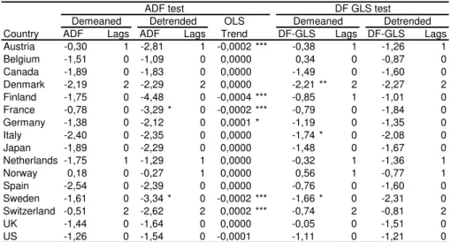
The results of PPP testing for RER based on unit labor cost and on

normal-ized unit labor cost are very similar. The ADF test does not detect stationarity

for any of the two series, as shown in Tables 4 and 5. Adding a trend to the

estimation results in the rejection of unit root for France for the two series, and

for Sweden for the unit labor cost series. The estimation with DF-GLS

some-what improves the results. Table 4 shows that the unit root null is rejected for

Denmark, Italy and Sweden, for the RER based on unit labor cost. For the

nor-malizes series, unit root is rejected only for Canada and Denamark, as presented

in Table 5. We cannot reject unit roots for any of the detrended estimations,

for the two sets of RER series. This means that no deterministic trend explain

the unit root evidence.

These results indicate that the RER proxied by the ratio of unit labor cost,

normalized or not, is a poor proxy for the relative prices of tradable goods. One

possible explanation is the fact the capital to labor ratio di¤ers substantially

across countries, so that the labor cost becomes a poor re‡ection of relative

The results for the value-added-RER series are interesting. The results from

ADF, in Table 6, detects no unit root. The DF-GLS, on the other hand,

re-jects the unit root null for …ve countries: France, Germany, Spain, Sweden and

Switzerland. These results, in Table 6, are close to the ones for the RER series

based on WPI, for which stationarity was found for six countries.

The worst results are those for the RER measures as a ratio of foreign

coun-tries CPI and domestic country WPI. No evidence of stationarity of theses series

were found, using both the ADF and the DF-GLS unit root tests, as shown by

the results presented in Table 7. This proxy for RER su¤ers from two of the

problems that could causes PPP deviations, as detected in equation (4): some

of the price indices have a large share of nontradable goods (the CPIs), and the

composition of foreign and domestic indices are substantially di¤erent (as we a

using simultaneously CPIs and WPIs)

Table 8 presents a summary of the results. The table presents the countries

for which we found evidence of PPP for each RER proxy and unit root test

used. The …rst striking result is that PPP is detected in a much larger set of

countries when we use the DF-GLS test, compared to the ADF test. This result

was expected. The DF-GLS has more power than the ADF, so that it is more

competent to reject the unit root null when the speed of convergence is low.

The RER proxy leader in stationarity is the one constructed as WPIs ratios,

presenting PPP evidence for six of the sixteen countries studied when we use

DF-GLS test with demeaned series. This is a signal that this price index is the

one that better …ts the requirement for PPP: more uniform goods composition

across countries and low share of nontradable goods. The second place goes

to the RER based on value added. PPP evidence was found for …ve of the

countries, for this RER proxy. The third position is a draw between the RER

based on export unit values and the one based on CPIs ratio: they both yield

to the RER constucted as the ratio between foreign countries CPIs and domestic

country WPI.

Looking at the countries’ perspective, France is the country for which PPP

evidence was found in the larger number of RER series. There is some evidence

of PPP for France for …ve of the seven RER proxies used. Switzerland and Italy

follow closely, with PPP evidence for four of the RER series. No evidence of

PPP was found in any of the series for …ve countries: Austria, Belgium, Japan,

United Kingdom and United States.

6

Concluding Remarks

There is a huge literature testing the PPP hypothesis, most of it using either

CPIs or WPIs ratios as proxies of relative currencies purchasing power, that

is, of the RER. Looking closely at the PPP argment, it states that the

cur-rencies purchasing power should not change when comparing the same basket

goods across countries, and these goods should all be tradable. Neither of those

price indices used in PPP testing fully satisfy these two criteria: they include

nontradable goods and their basket composition di¤ers across countries. We

observe that, if PPP is valid at all, it should be captured by the relative price

indices that best …ts these two festures. Hence, we ran a horse race among

six di¤erent price indices available from the IMF database to see which one

would yield higher PPP evidence. We used RER proxies measured as the ratio

of export unit values, wholesale prices, value added de‡ators, unit labor costs,

normalized unit labor costs and consumer prices. PPP was tested using both

the ADF and the DF-GLS unit root test of the RER series.

The RER measured as WPI ratios was the one for which PPP evidence was

found for the larger number of countries: six out of sixteen when we use

WPI seems to be the one with larger composition of tradable goods and with

least variation in its goods basket composition across countries.

The second best RER measure was the value added de‡ators. On the one

hand, this is an index that includes the cost of all factors of production. On the

other hand, the index composition may vary substantially across countries due

to the lack of cross-country comparability.

Unit labor costs and normalized unit labor cost proved to be poor measures

of tradable goods, as PPP evidence was found for a small number of countries,

when RER was measured by them. However, the worst measure of all was the

RER based on the ratio of foreign CPI and domestic WPI. No evidence of PPP

at all was found for this measure.

Finally, deterministic trends were found to be signi…cant in several cases,

possibly indicating some Balassa-Samuelson e¤ect.

Overall, this paper also identi…es the importance of the price index choice

to compute the RER for PPP testing. The results di¤ers substantially when

di¤erent proxies for the RER were used. Nevertheless, some consistency was

present. We found evidence for RER series for France, Switzerland and Italy

for most of the RER proxies, whereas no PPP evidence was found for Austria,

Belgium, Japan, United kingdom and United States for any of the proxies.

References

[1] Balassa, Bela, 1964, “The Purchasing Power Parity Doctrine: A

Reap-praisal,”Journal of Political Economy 72: 584-96.

[2] Cassel, Gustav, 1918, “Abnormal Deviations in International Exchanges,”

[3] Cheung, Yin-Wong and Kon S. Lai, 1998, “Parity Reversion in Real

Ex-change Rates during the Post-Bretton Woods Period,”Journal of

Interna-tional Money and Finance 17(4): 597-614.

[4] Chinn, Menzie, 1998, “Before the Fall: Were East Asian Currencies

Over-valued”,Emerging Markets Review 1 (2).

[5] De Gregorio, José, Alberto Giovannini and Holger C. Wolf, 1994,

“Interna-tional Evidence on Tradables and Nontradables In‡ation,” European

Eco-nomic Review 38(June).

[6] Dornbusch, Rudiger, 1987, “Purchasing Power Parity,” in John Eatwell,

Murray Milgate and Peter Newman (eds.)The New Palgrave: A Dictionary

of Economics, vol. 3: 1075-85 (New York: Stockton Press, 3rd ed.).

[7] Edwards, Sebastian, 1989,Real Exchange Rates, Devaluation and

Adjust-ment: Exchange Rate Policy in Developing Countries (Cambridge,

Massa-chusetts: MIT Press).

[8] Edwards, Sebastian, 1994, “Real and Monetary Determinants of Real

Ex-change Rate Behavior: Theory and Evidence from Developing Countries,”

in John Williamson (ed.) Estimating Equilibrium Exchange Rates

(Wash-ington: Institute for International Economics).

[9] Elbadawi, Ibrahim, 1994, “Estimating Long-Run Equilibrium Real

Ex-change Rates,” in John Williamson (ed.)Estimating Equilibrium Exchange

Rates (Washington: Institute for International Economics).

[10] Elliott, Graham, Thomas J. Rothenberg and James H. Stock, 1996,

“E¢-cient Tests for an Autoregressive Unit Root,”Econometrica64(4): 813-36.

[11] Frenkel, Jacob A., 1978, “Purchasing Power Parity: Doctrinal Perspective

[12] Froot, Kenneth A. and Kenneth Rogo¤, 1995, “Perspectives on PPP and

Long Run Real Exchange Rates,” in Gene M. Grossman and Kenneth

Rogo¤ (eds.) Handbook of International Economics, vol. 3 (Amsterdam:

North-Holland).

[13] International Monetary Fund, 1984, “Issues in the Assessment of the

Ex-change Rates of Industrial Countries”, IMF Occasional Paper No. 29.

[14] Ito, Takatoshi, Peter Isard, Steven Symansky and Tamim Bayoumi, 1996,

“Exchange Rate Movements and Their Impact in Trade and Investment in

the APEC Region”, IMF Occasional Paper No. 145.

[15] Keynes, John M., 1932, Essays in Persuasion (New York: Hartcourt

Brace).

[16] Rogo¤, Kenneth, 1996, “The Purchasing Power Parity Puzzle,”Journal of

Economic Literature 34: 647-68.

[17] Samuelson, Paul A., 1964, “Theoretical Notes on Trade Problems”,Review

of Economics and Statistics 46: 145-54.

[18] Sarno, Lucio and Taylor, Mark P., 2002, “Purchasing Power Parity and

the Real Exchange Rate”, IMF Sta¤ Papers vol. 49, No 1 (Washington:

International Monetary Fund).

[19] Taylor, Alan N., 2002, “A Century of Purchasing-Power Parity,”Review of

Economics and Statistics 84(1): 139-50.

7

Appendix

This appendix presents the methodologies for computation of weights(Wij)that

We begin with the methodology for the weights used in the computation

of RER based on relative export unit values, wholesale prices, value added

de‡ators, unit labor costs and normalized unit labor costs.

From January 1991 onwards, Wij uses data on trade and consumption of

manufactured goods over the period 1989-91. Before that, the weights used in

the computation of MRER were based on 1980 data.

Let there be k markets in which the producers of countryi and countryj

compete. LetTk

l represent the sales of countrylin marketk:Letskj be country

j0smarket share in marketkandwki be the share of countryi0soutput sold in

marketk; which is to say:

skj =

Tjk

P

l

Tk l

and (9)

wki =

Tk i P n Tn i : (10)

Then, the weight attached to countryj by countryiis:

Wij =

P

k

wk iskj

P

k

wk i(1 s

k i)

: (11)

This weight can be interpreted as the sum over all markets of a gauge of

the degree of competition between producers of countriesiandjdivided by the sum over all markets of a gauge of the degree of competition between producers

of countryi and all other producers.

The world is divided into 22 markets, the …rst 21 markets being the

coun-tries2 _{for which MRER were being computed by IMF and the last market is} 2_{These 21 countries are Australia, Austria, Belgium, Canada, denmark, Finland, France,}

called ”Rest-of-the-World”.

Next we will present the second methodology that describes the weights used

in the computation of MRER based on consumer price index.

From January 1990 onwards, Wij is weighted by a set of weights based on

trade in manufactures, non-oil primary commodities and, for a set of 46 countries

and regions3 _{in which services accounted to meet more than 20 percent of all}

exports in 1989-90, tourism services covering the three-year period 1988-1990.

Prior to January 1990, the weights are for the three-year span 1980-82.

These weights are then aggregated to derive the overall weight attached by

countryi to countryj,Wij: Speci…cally:

Wij= i(M)Wij(M) + i(P)Wij(P) + i(T)Wij(T); (12)

where Wij(M); Wij(P) and Wij(T) are weights based on trade in

manufac-tures, primary commodities and tourism services. The factors i(M); i(P)

and i(T) are the shares of trade in manufactures, primary commodities and

tourism services in country i0s external trade, with external computed as the sum of trade in manufactures, primary commodities and tourism services.

Ob-serve that i(T) = 0for a set of countries in which services accounted to meet

less than 20 percent of all exports in 1989-90. For these countries, i(M)and i(P)are the shares of trade in manufactures and primary commodities in

to-tal trade, with toto-tal trade being computed as the sum of trade in these two

categories.

The weights based on trade in manufactures, Wij(M); and on trade in

tourism,Wij(T);are computed in a manner analogous to equation (11). These

3_{These 46 countries and regions are Antigua and Borbuda, Austria, The Bahamas,}

weights are a weighted sum of a weight re‡ecting competition in the domestic

market, a weight re‡ecting competition abroad against domestic producers and

a weight re‡ecting competition abroad against exporters.

The weights based on trade in primary commodities,Wij(P);are computed

in a very di¤erent way. Contrary to manufactured goods and tourism services,

primary commodities are assumed to be homogeneous goods. Then, for each

commodity, the weight attached to country j by any country should re‡ect the importance of countryj as either a seller or a buyer in the world market. Therefore, for countryi;the weight attached to countryj; Wij(P);should be a

(normalized) sum over all commodity markets of the product of the individual

Table 1: ADF and DF-GLS tests: RER based on export unit value

OLS

Country ADF Lags ADF Lags Trend DF-GLS Lags DF-GLS Lags Austria -2,12 4 -2,11 4 0,0000 -0,34 4 -1,44 4 Belgium -2,55 0 -2,20 0 0,0000 -0,94 0 -1,58 0 Canada -0,31 0 -2,40 0 -0,0002 ** 1,53 0 -2,46 0 Denmark -1,20 0 -1,52 0 0,0000 -1,22 0 -1,32 0 Finland -2,19 0 -2,14 0 0,0000 -0,68 0 -1,74 0 France -2,61 * 0 -2,90 0 0,0000 -2,60 *** 0 -2,87 * 0 Germany -1,77 0 -1,93 0 0,0000 -1,75 * 0 -2,02 0 Italy -2,41 0 -2,43 0 0,0000 -2,36 ** 0 -2,46 0 Japan -1,21 0 -1,74 0 0,0001 -1,21 0 -1,48 0 Netherlands -2,42 0 -2,54 0 0,0000 -2,04 ** 0 -2,23 0 Norway -2,49 1 -2,79 1 -0,0001 -0,94 1 -2,43 1 Spain -1,30 0 -2,15 0 0,0001 * -1,25 0 -1,79 0 Sweden -2,69 0 -2,43 0 0,0000 -1,06 0 -1,76 0 Switzerland -1,06 0 -3,40 * 0 0,0004 *** -0,12 0 -3,32 ** 0 UK -2,13 0 -2,64 0 0,0001 -0,81 0 -2,48 0 US -1,51 0 -1,50 0 0,0000 -0,69 0 -1,19 0 Notes: Data from 1975:1 to 1998:2. The lag length is selected by Modified SIC, with maximal lag length equal to 6. Asterisks denotes significance at the *10%, **5%, and ***1% levels. The ADF test critical values corresponding to these significance levels are (-2,58, -2,89, -3,51) for the demeaned series and (-3,16, -3,46, -4,06) for the detrended series, respectively. The DF-GLS test critical values corresponding to these significance levels are (-1,61, -1,94, -2,59) for the demeaned series and (-2,77, -3,07, -3,62) for the detrended series, respectively.

Detrended DF GLS test Demeaned Detrended Demeaned

ADF test

Table 2: ADF and DF-GLS tests: RER based on wholesale price index

OLS

Country ADF Lags ADF Lags Trend DF-GLS Lags DF-GLS Lags Austria -1,58 2 -2,63 2 -0,0001 ** -1,51 2 -2,37 2 Belgium -1,38 1 -1,10 0 0,0000 -0,02 1 -1,08 0 Canada -1,88 0 -1,77 0 0,0000 -1,04 0 -1,56 0 Denmark -1,51 0 -1,83 0 0,0000 -1,52 0 -1,65 0 Finland -1,30 0 -1,46 0 0,0000 -1,71 * 1 -1,50 0 France -1,83 0 -1,92 0 0,0000 -1,74 * 0 -1,80 0 Germany -1,69 0 -2,08 0 0,0000 -1,69 * 0 -1,86 0 Italy -1,90 0 -1,92 0 0,0000 -1,89 * 0 -1,95 0 Japan -1,57 0 -1,71 0 0,0001 -1,59 1 -1,86 0 Netherlands -1,39 0 -1,54 0 0,0000 -1,39 0 -1,45 0 Norway -1,51 0 -0,58 0 0,0000 -0,52 0 -0,92 0 Spain -2,21 0 -2,16 0 0,0000 -2,21 ** 0 -2,22 0 Sweden -2,30 0 -2,23 0 0,0000 -1,52 0 -2,03 0 Switzerland -2,47 0 -2,70 0 0,0001 -2,49 ** 0 -2,65 0 UK -1,77 0 -2,22 0 0,0001 -0,50 0 -2,09 0 US -1,12 0 -1,57 0 -0,0001 -1,22 0 -1,40 0 Notes: Data from 1975:1 to 1997:1. The lag length is selected by Modified SIC, with maximal lag length equal to 6. Asterisks denotes significance at the *10%, **5%, and ***1% levels. The ADF test critical values corresponding to these significance levels are (-2,58, -2,90, -3,51) for the demeaned series and (-3,16, -3,46, -4,07) for the detrended series, respectively. The DF-GLS test critical values corresponding to these significance levels are (-1,61, -1,94, -2,59) for the demeaned series and (-2,78, -3,07, -3,63) for the detrended series, respectively.

Table 3: ADF and DF-GLS tests: RER based on consumer price index

OLS

Country ADF Lags ADF Lags Trend DF-GLS Lags DF-GLS Lags Austria -1,52 0 -1,59 0 0,0000 -0,74 0 -1,66 0 Belgium -1,63 1 -1,76 1 0,0000 -0,90 1 -1,75 1 Canada -1,13 1 -1,58 0 -0,0001 -0,20 1 -1,59 0 Denmark -1,85 0 -2,13 0 0,0000 -1,81 * 0 -1,90 0 Finland -1,64 1 -1,55 0 0,0000 -1,64 * 1 -1,37 0 France -1,63 0 -2,26 0 0,0000 -0,61 0 -2,25 0 Germany -2,00 0 -1,94 0 0,0000 -0,81 1 -1,54 0 Italy -2,00 1 -1,47 0 0,0000 -1,98 ** 1 -2,07 1 Japan -2,08 1 -1,79 0 0,0001 -0,71 1 -1,72 0 Netherlands -1,76 0 -1,73 0 0,0000 -1,16 0 -1,82 0 Norway -1,97 0 -1,65 0 0,0000 -1,64 * 0 -1,93 0 Spain -1,84 0 -1,73 0 0,0000 -1,22 0 -1,62 0 Sweden -1,10 0 -2,12 0 -0,0001 * 0,01 0 -2,16 0 Switzerland -2,12 0 -2,89 0 0,0001 * -1,45 0 -2,91 * 0 UK -1,69 0 -1,95 0 0,0001 -1,09 0 -1,97 0 US -1,04 0 -1,08 0 0,0000 -0,92 0 -1,16 0 Notes: Data from 1975:1 to 2002:3. The lag length is selected by Modified SIC, with maximal lag length equal to 6. Asterisks denotes significance at the *10%, **5%, and ***1% levels. The ADF test critical values corresponding to these significance levels are (-2,58, -2,89, -3,49) for the demeaned series and (-3,15, -3,45, -4,04) for the detrended series, respectively. The DF-GLS test critical values corresponding to these significance levels are (-1,61, -1,94, -2,59) for the demeaned series and (-2,73, -3,02, -3,57) for the detrended series, respectively.

ADF test DF GLS test Demeaned Detrended Demeaned Detrended

Table 4: ADF and DF-GLS tests: RER based on unit labor cost

OLS

Country ADF Lags ADF Lags Trend DF-GLS Lags DF-GLS Lags Austria -0,30 1 -2,81 1 -0,0002 *** -0,38 1 -1,26 1 Belgium -1,51 0 -1,09 0 0,0000 0,34 0 -0,87 0 Canada -1,89 0 -1,83 0 0,0000 -1,49 0 -1,60 0 Denmark -2,19 2 -2,29 2 0,0000 -2,21 ** 2 -2,27 2 Finland -1,75 0 -4,48 0 -0,0004 *** -0,85 1 -1,01 0 France -0,78 0 -3,29 * 0 -0,0002 *** -0,79 0 -1,84 0 Germany -1,38 0 -2,12 0 0,0001 * -1,19 0 -1,35 0 Italy -2,40 0 -2,35 0 0,0000 -1,74 * 0 -2,08 0 Japan -1,89 0 -2,29 0 0,0000 -1,48 0 -1,67 0 Netherlands -1,75 1 -1,29 1 0,0000 -0,32 1 -1,36 1 Norway 0,18 0 -0,27 1 0,0000 0,56 1 -0,77 1 Spain -2,54 0 -2,39 0 0,0000 -0,76 0 -1,60 0 Sweden -1,61 0 -3,34 * 0 -0,0002 *** -1,66 * 0 -2,31 0 Switzerland -0,51 2 -2,62 2 0,0002 *** -0,74 2 -0,81 2 UK -1,44 0 -1,64 0 0,0000 -0,05 0 -1,51 0 US -1,26 0 -1,54 0 -0,0001 -1,11 0 -1,21 0 Notes: Data from 1975:1 to 2002:3. The lag length is selected by Modified SIC, with maximal lag length equal to 6. Asterisks denotes significance at the *10%, **5%, and ***1% levels. The ADF test critical values corresponding to these significance levels are (-2,58, -2,89, -3,49) for the demeaned series and (-3,15, -3,45, -4,04) for the detrended series, respectively. The DF-GLS test critical values corresponding to these significance levels are (-1,61, -1,94, -2,59) for the demeaned series and (-2,73, -3,02, -3,57) for the detrended series, respectively.

Table 5: ADF and DF-GLS tests: RER based on normalized unit labor cost

OLS

Country ADF Lags ADF Lags Trend DF-GLS Lags DF-GLS Lags Austria -0,55 0 -2,79 1 -0,0002 *** -0,53 0 -1,38 1 Belgium -2,10 0 -1,37 0 0,0000 0,71 1 -0,87 0 Canada -2,00 1 -2,07 1 0,0000 -1,80 * 1 -1,90 1 Denmark -2,34 0 -2,56 0 0,0000 -2,32 * 0 -2,41 0 Finland -1,30 0 -4,09 0 -0,0004 *** -0,83 0 -0,98 0 France -0,38 0 -3,44 * 0 -0,0002 *** -0,42 0 -1,55 0 Germany -1,22 0 -2,14 0 0,0001 * -1,14 0 -1,32 0 Italy -2,45 0 -2,39 0 0,0000 -1,56 0 -1,96 0 Japan -1,91 0 -2,39 0 0,0001 -1,50 0 -1,70 0 Netherlands -1,75 0 -1,20 0 0,0000 0,07 0 -1,21 0 Norway -1,15 1 0,01 0 0,0001 1,30 1 -0,38 0 Spain -2,48 0 -2,44 0 0,0000 -0,83 0 -1,91 0 Sweden -1,15 0 -3,01 0 -0,0002 *** -1,56 0 -2,40 0 Switzerland -0,43 2 -2,51 2 0,0002 *** -0,68 2 -0,88 2 UK -1,18 0 -1,64 0 0,0000 0,07 0 -1,61 0 US -1,25 0 -1,57 0 -0,0001 -1,02 0 -1,15 0 Notes: Data from 1975:1 to 2002:3. The lag length is selected by Modified SIC, with maximal lag length equal to 6. Asterisks denotes significance at the *10%, **5%, and ***1% levels. The ADF test critical values corresponding to these significance levels are (-2,58, -2,89, -3,49) for the demeaned series and (-3,15, -3,45, -4,04) for the detrended series, respectively. The DF-GLS test critical values corresponding to these significance levels are (-1,61, -1,94, -2,59) for the demeaned series and (-2,73, -3,02, -3,57) for the detrended series, respectively.

ADF test DF GLS test Demeaned Detrended Demeaned Detrended

Table 6: ADF and DF-GLS tests: RER based on value added

OLS

Country ADF Lags ADF Lags Trend DF-GLS Lags DF-GLS Lags Austria -1,42 4 -2,30 3 -0,0002 ** -0,99 4 -1,90 3 Belgium -1,73 0 -1,04 0 0,0000 -0,85 4 -0,83 0 Canada -1,65 1 -1,69 0 0,0000 -1,46 0 -1,55 0 Denmark -0,35 0 -1,62 0 0,0001 * -0,27 0 -1,19 0 Finland -0,92 0 -1,57 0 -0,0001 -0,69 0 -1,54 0 France -2,05 0 -2,14 0 0,0000 -2,00 ** 0 -2,17 0 Germany -2,06 6 -2,02 3 0,0001 -1,84 * 6 -2,05 3 Italy -1,82 0 -1,81 0 0,0000 -1,52 0 -1,78 0 Japan -2,06 1 -1,65 0 0,0001 -1,20 1 -1,80 0 Netherlands -2,09 0 -1,76 0 0,0000 -0,53 0 -1,33 0 Norway -1,45 0 -2,28 0 0,0001 -1,57 0 -2,26 0 Spain -2,21 0 -2,27 0 0,0001 -1,63 * 0 -2,31 0 Sweden -2,33 0 -2,27 0 0,0000 -1,65 * 0 -2,08 0 Switzerland -2,92 0 -2,94 0 0,0000 -2,92 *** 0 -3,00 * 0 UK -1,75 0 -1,77 0 0,0000 -0,60 0 -1,57 0 US -1,08 0 -1,57 0 -0,0001 -0,84 0 -1,50 0 Notes: Data from 1975:1 to 1997:1. The lag length is selected by Modified SIC, with maximal lag length equal to 6. Asterisks denotes significance at the *10%, **5%, and ***1% levels. The ADF test critical values corresponding to these significance levels are (-2,59, -2,90, -3,51) for the demeaned series and (-3,16, -3,46, -4,07) for the detrended series, respectively. The DF-GLS test critical values corresponding to these significance levels are (-1,61, -1,94, -2,59) for the demeaned series and (-2,79, -3,08, -3,64) for the detrended series, respectively.

Table 7: ADF and DF-GLS tests: RER based on CPI over WPI

OLS

Country ADF Lags ADF Lags Trend DF-GLS Lags DF-GLS Lags Austria -0,01 1 -1,47 0 0,0001 0,69 2 -1,36 0 Belgium -0,80 1 -1,59 1 0,0001 * -0,66 1 -1,53 1 Canada -1,49 1 -1,38 1 0,0000 -1,51 1 -1,50 1 Denmark -1,72 0 -1,88 0 0,0000 -1,55 0 -1,64 0 Finland -1,42 0 -1,61 0 0,0000 -0,35 0 -1,60 0 France -0,71 0 -1,70 0 0,0001 -0,43 0 -1,57 0 Germany -0,96 1 -1,51 0 0,0001 * -0,91 1 -1,86 1 Italy -1,10 1 -1,92 0 0,0002 * -0,59 1 -1,81 0 Japan -1,38 1 -1,81 0 0,0002 -0,16 1 -1,84 0 Netherlands -1,00 1 -1,25 0 0,0001 -0,70 1 -1,30 0 Norway -1,16 1 -1,33 0 0,0001 -0,87 1 -1,36 0 Spain -1,04 1 -1,32 0 0,0001 -0,79 1 -1,34 0 Sweden -1,12 1 -1,25 0 0,0001 -0,92 1 -1,27 0 Switzerland -0,75 1 -1,20 0 0,0001 -0,48 1 -1,21 0 UK -0,82 1 -1,25 0 0,0001 -0,52 1 -1,27 0 US -0,92 0 -1,38 0 0,0001 -0,93 0 -1,41 0 Notes: Data from 1975:1 to 1998:4. The lag length is selected by Modified SIC, with maximal lag length equal to 6. Asterisks denotes significance at the *10%, **5%, and ***1% levels. The ADF test critical values corresponding to these significance levels are (-2,58, -2,89, -3,50) for the demeaned series and (-3,15, -3,46, -4,06) for the detrended series, respectively. The DF-GLS test critical values corresponding to these significance levels are (-1,61, -1,94, -2,59) for the demeaned series and (-2,79, -3,08, -3,64) for the detrended series, respectively.

Tabela 8: Countries with PPP evidence

RER Proxy Demeaned Detrended Demeaned Detrended

Exp. unit v. France Switzerland France France

Sweden Germany Switzerland

Italy Netherlands

WPI - - Finland

-France Germany

Italy Spain Switzerland

CPI - Denmark Switzerland

Finland Italy Norway

Labor u. c. - France Denmark

-Sweden Italy

Sweden

Norm. l. u. v. - France Canada

-Denmark

Value add. Switzerland - France Switzerland

Germany Spain Sweden Switzerland

CPI/WPI - - -

´

Ultimos Ensaios Econˆomicos da EPGE

[594] Pedro Cavalcanti Gomes Ferreira, Roberto de G´oes Ellery Junior, e Victor Go-mes. Produtividade Agregada Brasileira (1970–2000): decl´ınio robusto e fraca recuperac¸˜ao. Ensaios Econˆomicos da EPGE 594, EPGE–FGV, Jul 2005.

[595] Carlos Eugˆenio Ellery Lustosa da Costa e Lucas J´over Maestri. The Interac-tion Between Unemployment Insurance and Human Capital Policies. Ensaios Econˆomicos da EPGE 595, EPGE–FGV, Jul 2005.

[596] Carlos Eugˆenio Ellery Lustosa da Costa. Yet Another Reason to Tax Goods. Ensaios Econˆomicos da EPGE 596, EPGE–FGV, Jul 2005.

[597] Marco Antonio Cesar Bonomo e Maria Cristina Trindade Terra.Special Interests and Political Business Cycles. Ensaios Econˆomicos da EPGE 597, EPGE–FGV, Ago 2005.

[598] Renato Galv˜ao Flˆores Junior. Investimento Direto Estrangeiro no Mercosul: Uma Vis˜ao Geral. Ensaios Econˆomicos da EPGE 598, EPGE–FGV, Ago 2005.

[599] Aloisio Pessoa de Ara´ujo e Bruno Funchal. Past and Future of the Bankruptcy Law in Brazil and Latin America. Ensaios Econˆomicos da EPGE 599, EPGE– FGV, Ago 2005.

[600] Marco Antonio Cesar Bonomo e Carlos Carvalho. Imperfectly Credible Disin-flation under Endogenous Time–Dependent Pricing. Ensaios Econˆomicos da EPGE 600, EPGE–FGV, Ago 2005.

[601] Pedro Cavalcanti Gomes Ferreira. Sobre a Inexistente Relac¸˜ao entre Pol´ıtica Industrial e Com´ercio Exterior. Ensaios Econˆomicos da EPGE 601, EPGE– FGV, Set 2005.

[602] Luiz Renato Regis de Oliveira Lima, Raquel Sampaio, e Wagner Gaglianone.

Limite de Endividamento e Sustentabilidade Fiscal no Brasil: Uma abordagem via modelo Quant´ılico Auto–Regressivo (QAR). Ensaios Econˆomicos da EPGE 602, EPGE–FGV, Out 2005.

[603] Ricardo de Oliveira Cavalcanti e Ed Nosal.Some Benefits of Cyclical Monetary Policy. Ensaios Econˆomicos da EPGE 603, EPGE–FGV, Out 2005.

[604] Pedro Cavalcanti Gomes Ferreira e Leandro Gonc¸alves do Nascimento.Welfare and Growth Effects of Alternative Fiscal Rules for Infrastructure Investment in Brazil. Ensaios Econˆomicos da EPGE 604, EPGE–FGV, Nov 2005.

[606] Marcelo Cˆortes Neri, Luisa Carvalhaes, e Alessandra Pieroni. Inclus˜ao Digital e Redistribuic¸˜ao Privada. Ensaios Econˆomicos da EPGE 606, EPGE–FGV, Dez 2005.

[607] Marcelo Cˆortes Neri e Rodrigo Leandro de Moura. La institucionalidad del salario m´ınimo en Brasil. Ensaios Econˆomicos da EPGE 607, EPGE–FGV, Dez 2005.

[608] Marcelo Cˆortes Neri e Andr´e Luiz Medrado. Experimentando Microcr´edito: Uma An´alise do Impacto do CrediAMIGO sobre Acesso a Cr´edito. Ensaios Econˆomicos da EPGE 608, EPGE–FGV, Dez 2005.

[609] Samuel de Abreu Pessˆoa. Perspectivas de Crescimento no Longo Prazo para o Brasil: Quest˜oes em Aberto. Ensaios Econˆomicos da EPGE 609, EPGE–FGV, Jan 2006.

[610] Renato Galv˜ao Flˆores Junior e Masakazu Watanuki. Integration Options for Mercosul – An Investigation Using the AMIDA Model. Ensaios Econˆomicos da EPGE 610, EPGE–FGV, Jan 2006.

[611] Rubens Penha Cysne. Income Inequality in a Job–Search Model With Hetero-geneous Discount Factors (Revised Version, Forthcoming 2006, Revista Econo-mia). Ensaios Econˆomicos da EPGE 611, EPGE–FGV, Jan 2006.

[612] Rubens Penha Cysne. An Intra–Household Approach to the Welfare Costs of Inflation (Revised Version, Forthcoming 2006, Estudos Econˆomicos). Ensaios Econˆomicos da EPGE 612, EPGE–FGV, Jan 2006.

[613] Pedro Cavalcanti Gomes Ferreira e Carlos Hamilton Vasconcelos Ara´ujo. On the Economic and Fiscal Effects of Infrastructure Investment in Brazil. Ensaios Econˆomicos da EPGE 613, EPGE–FGV, Mar 2006.

[614] Aloisio Pessoa de Ara´ujo, Mario R. P´ascoa, e Juan Pablo Torres-Mart´ınez. Bub-bles, Collateral and Monetary Equilibrium. Ensaios Econˆomicos da EPGE 614, EPGE–FGV, Abr 2006.

[615] Aloisio Pessoa de Ara´ujo e Bruno Funchal. How much debtors’ punishment?. Ensaios Econˆomicos da EPGE 615, EPGE–FGV, Mai 2006.

[616] Paulo Klinger Monteiro. First–Price Auction Symmetric Equilibria with a Ge-neral Distribution. Ensaios Econˆomicos da EPGE 616, EPGE–FGV, Mai 2006.

[617] Renato Galv˜ao Flˆores Junior e Masakazu Watanuki.Is China a Northern Partner to Mercosul?. Ensaios Econˆomicos da EPGE 617, EPGE–FGV, Jun 2006.

[618] Renato Galv˜ao Flˆores Junior, Maria Paula Fontoura, e Rog´erio Guerra Santos.