Velocity fluctuations in polar solar wind: a comparison between different solar cycles

www.ann-geophys.net/27/877/2009/

© Author(s) 2009. This work is distributed under the Creative Commons Attribution 3.0 License.

Annales

Geophysicae

Velocity fluctuations in polar solar wind: a comparison between

different solar cycles

B. Bavassano, R. Bruno, and R. D’Amicis

Istituto di Fisica dello Spazio Interplanetario, Istituto Nazionale di Astrofisica, Roma, Italy

Received: 8 October 2008 – Revised: 26 January 2009 – Accepted: 4 February 2009 – Published: 20 February 2009

Abstract.The polar solar wind is a fast, tenuous and steady flow that, with the exception of a relatively short phase around the Sun’s activity maximum, fills the high-latitude heliosphere. The polar wind properties have been exten-sively investigated by Ulysses, the first spacecraft able to per-form in-situ measurements in the high-latitude heliosphere. The out-of-ecliptic phases of Ulysses cover about seventeen years. This makes possible to study heliospheric properties at high latitudes in different solar cycles. In the present in-vestigation we focus on hourly- to daily-scale fluctuations of the polar wind velocity. Though the polar wind is a quite uniform flow, fluctuations in its velocity do not appear negli-gible. A simple way to characterize wind velocity variations is that of performing a multi-scale statistical analysis of the wind velocity differences. Our analysis is based on the com-putation of velocity differences at different time lags and the evaluation of statistical quantities (mean, standard deviation, skewness, and kurtosis) for the different ensembles. The re-sults clearly show that, though differences exist in the three-dimensional structure of the heliosphere between the inves-tigated solar cycles, the velocity fluctuations in the core of polar coronal holes exhibit essentially unchanged statistical properties.

Keywords. Interplanetary physics (MHD waves and turbu-lence; Solar wind plasma; Sources of the solar wind)

1 Introduction

The polar solar wind is a fast plasma flow coming from po-lar coronal holes. With the exception of a relatively short phase around the Sun’s activity maximum, the polar wind is

Correspondence to:B. Bavassano (bavassano@ifsi-roma.inaf.it)

a dominant feature of the high-latitude heliosphere. Its prop-erties have been extensively investigated by Ulysses, the first spacecraft with a highly inclined orbital plane with respect to the ecliptic. Launched in October 1990, the Ulysses’ out-of-ecliptic journey began in February 1992, with a Jupiter grav-ity assist. Presently data extend till December 2008, though the spacecraft operations were expected to end in July 2008 (due to technical problems arisen in January 2008). With an orbital period of 6.2 years, during this period of time Ulysses has covered two complete out-of-ecliptic orbits and∼_78% of the third one. However, during 2008 the data coverage suffered a strong decline.

Ulysses had its first polar passes in 1994 (South) and 1995 (North), during the declining phase of solar cycle 22. In con-trast, the second set of polar passes in 2000–2001 occurred at high solar activity. During the 1994–1995 polar passes Ulysses found an ordered heliosphere, with clear differences between the solar wind near the poles (polar wind) and that around the equator (McComas et al., 2000). Near solar max-imum (2000–2001) things were more complex, making it hard to distinguish any particular region from another (Mc-Comas et al., 2003). For the third set of polar passes in 2006– 2008, during cycle 23, the solar activity was again low and the polar wind was again present at the high latitudes (McCo-mas et al., 2008). These new polar wind observations offer the opportunity of investigating, by comparison with those from the first orbit, if the polar wind properties vary between consecutive solar cycles, with reversal of the Sun’s magnetic field polarity, namely along the∼22-year Hale magnetic cy-cle.

0o _-30o _-60o _-90o _-60o _-30o ₀o ₃₀o ₆₀o ₉₀o ₆₀o ₃₀o ₀o 400

500 600 700 800

(km/s)

V

South

North

0o _-30o _-60o _-90o _-60o _-30o ₀o ₃₀o ₆₀o ₉₀o ₆₀o ₃₀o ₀o 400

500 600 700 800

(km/s)

V

South

North

Fig. 1.Magnitude of the solar wind velocityV vs. latitudeλduring the first (top) and third (bottom) out-of-ecliptic orbit of Ulysses. Zero latitude at the left and right ends corresponds to the aphelion solar equator crossing, that in the center is for the near-perihelion crossing. Blue and red horizontal segments indicate the analysed intervals (see text). The velocity decrease highlighted by green arrows in the bottom panel is caused by the tail of comet Mc-Naught.

larger average tilt and a non-planar shape. Hence, not sur-prisingly, in the third orbit of Ulysses the polar wind ap-pears less extended in latitude, slightly slower, less dense, and cooler than in the first orbit (note that these trends lead to a lower dynamic pressure of the wind in the third orbit). Mc-Comas et al. (2008) have stressed that measurements in the near-ecliptic wind, while much more variable, match quanti-tatively with those by Ulysses and show essentially identical trends. Thus, the entire Sun appears involved in long-term changes of the solar wind output.

Though the polar solar wind is a relatively steady flow, as compared to low latitude conditions, fluctuations in its veloc-ity magnitudeV are not negligible. The goal of present anal-ysis is of comparing, between cycles 22 and 23, the proper-ties ofV variations at time scales between 1 h and∼10 days. With this choice we cover fluctuations from scales at which a turbulent regime is typically developed in the wind up to scales at which high-latitude microstreams (Neugebauer et al., 1995) become a dominant feature. In other words, at the short scales we are looking at variations mainly caused by a turbulent cascade, while at the long scales variations should

Table 1.Data intervals used to derive solar-rotation distributions of

V: start and end times (year, day, hour), minimum and maximum

distances (R, in AU), and latitudes (λ, in degrees, with n and s for North and South, respectively).

interval time R λ

min max min max

South 1 1994 015 05 – 1994 356 05 1.61 – 3.76 49.7s – 80.2s North 1 1995 118 12 – 1996 094 22 1.44 – 3.59 41.3n – 80.2n South 3 2006 165 17 – 2007 141 12 1.69 – 3.77 50.9s – 79.8s North 3 2007 281 10 – 2008 257 06 1.50 – 3.58 42.3n – 79.8n

be mainly related to conditions at the source solar region and to propagation effects. Changes in power spectra (Bavassano et al., 2005) across the scales investigated here are indicative of the different nature of the velocity variations. Following Burlaga and Forman (2002), to characterize these variations a multi-scale statistical analysis of the velocity differences will be used.

2 The analysed Ulysses data

Figure 1 shows daily averages of solar wind velocity magni-tudeV vs. heliographic latitudeλduring the first (top) and third (bottom) out-of-ecliptic orbit. Zero values of latitude at the left and right ends correspond to the solar equator cross-ing near the aphelion (5.41 AU, astronomical unit), while that in the center corresponds to the perihelion (1.34 AU) equato-rial crossing. Near the aphelion, only data at latitudes greater than 10◦_{, in absolute value, have been plotted. The curve}

in the bottom panel ends with the latest available data at the time of paper final version. Note that the velocity drop indi-cated by green arrows around the maximum southern latitude of the third orbit is caused by an encounter of Ulysses with the comet McNaught tail (Neugebauer et al., 2007).

650 700 750 800 850

(km/s)

rot Classes

V

F (%) 0 5 10 15 20 25 30

-80o -70o

-60o -50o

South 1

650 700 750 800 850

(km/s)

rot Classes

V

2 4 6 8 10 12

650 700 750 800 850

(km/s)

rotation number

V

40o

50o

60o

70o

80o

North 1

-80o

-70o

-60o -50o

South 3

12 10 8 6 4 2 650 700 750 800 850

(km/s)

rotation number

V

40o

50o

60o

70o

80o

North 3

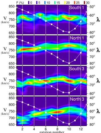
Fig. 2. Two-dimensional plots ofV distributions vs. solar rota-tion. Colours give the occurrence frequency (in per cent, see colour scale on top) for each velocity bin (width 10 km/s) at each rota-tion. Superposed white squares indicate the rotation average

lati-tudeλ(right y-axis). From top to bottom: southern and northern

phase of the first orbit (South 1 and North 1) and of the third orbit (South 3 and North 3).

intervals correspond to latitudes poleward of∼40◦

(∼50◦

) in the Northern (Southern) Hemisphere, respectively.

Figure 2 shows 2-D plots of the thirteen distributions of wind velocity versus rotation number. These plots are ob-tained by computing, for each rotation, the occurrence dis-tribution ofV (hourly values) and building a matrix with a column for each distribution. In this way a comparison be-tween different rotations (or, columns) is easily performed. Superposed white squares give the average latitude for each rotation. The South 1 and North 1 (South 3 and North 3) panels are for the southern and northern phase of the first (third) orbit, respectively. Note that South 3 data do not in-clude those from the comet McNaught encounter. As already stressed by McComas et al. (2000), for the first orbit the po-lar wind is more regupo-lar in the Northern Hemisphere (panel North 1). Here the velocity distributions vary in a smooth way versus the rotation number, with a regular increase in velocity for increasing latitude. In the Southern Hemisphere (South 1) this trend is less clear and variations between

con-Table 2.Data intervals used for the multi-scale analysis of velocity differences: start and end times (year, day, hour), minimum and maximum distances (R, in AU), and latitudes (λ, in degrees, with n and s for North and South, respectively).

interval time R λ

min max min max

S1 1994 176 06 – 1994 256 18 2.29 – 2.84 69.8s – 80.2s N1 1995 189 21 – 1995 273 08 1.86 – 2.44 69.8n – 80.2n S3 2006 320 19 – 2007 035 22 2.39 – 2.91 69.8s – 79.7s N3 2007 357 12 – 2008 075 12 1.93 – 2.50 69.8n – 79.8n

secutive rotations may be relevant. As regards the third orbit, for both South 3 and North 3 intervals the distributions are shifted to lower velocities. However, the main belt, repre-senting the great majority of the velocity values, maintains a shape similar to that of the first orbit samples. At the same time it is easily seen how the polar wind is confined to higher latitudes, especially for distributions of the North 3 panel.

3 Wind velocity structure at very high latitude

A simple way to characterize the solar wind structure is that of performing a multi-scale statistical analysis of the velocity variations. Following Burlaga and Forman (2002), our anal-ysis is based on 1) the computation of velocity differences at different time lags and 2) the evaluation of statistical quan-tities for the resulting ensembles. More specifically, starting from the time series ofV hourly averages, we have first de-rived a set of time series of velocity differencesδV n(t ) at time lagsτ=2n(t andτ in hours) as

δV n≡δV n(t )=V (t+₂n)−V (t )

10 20 30 40

St.

Dev.

(km/s)

S1

N1

S3

N3

-0.5 0 0.5 1 1.5 2

Skewness

1 2 4 8 16 32 64 128 256 0

5 10 15 20

(hours)

Kurtosis

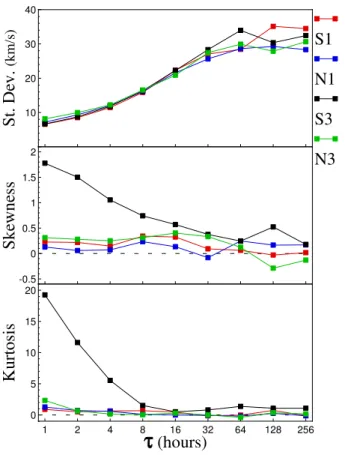
Fig. 3.From top to bottom: standard deviation, skewness, and

kur-tosis versus time lagτ for the intervals of Table 2. Error bars for

skewness and kurtosis are not appreciably larger than the marker size.

widely used as a measure of non-Gaussianity, skewness and kurtosis have some drawbacks when estimated from experi-mental observations. The main problem is that they can be very sensitive to outliers, in other words their values may de-pend on only few observations in the tails of the distribution, which might be erroneous or irrelevant observations.

Multi-scale statistical analyses of velocity differences for the ecliptic solar wind have been performed by Burlaga and Forman (2002) and Burlaga et al. (2003), and for the polar wind by Bavassano et al. (2005) (see also Bavassano et al., 2004, for a comparison between high-latitude and ecliptic wind at solar maximum). Here we focus on a comparison be-tween polar wind in different solar cycles. It has been shown above that the latitudinal extent of the polar wind changes with the solar cycle. In order to avoid effects caused by dif-ferences in the location of the polar wind low-latitude bound-ary, for our multi-scale analysis we will use data intervals well in the core of the heliospheric region filled by the polar wind. In other words we will analyse data intervals at very high latitude. A problem with this choice is represented by the velocity drop caused by the comet McNaught just near the maximum southern latitude of the Ulysses’ third orbit.

700 750 800 850

(km/s)

V

-50 0 50

(km/s)

V0

=1h

-50 0 50

(km/s)

V1

=2h

-50 0 50

(km/s)

V2

=4h

-50 0 50

(km/s)

V5

=32h

320 340 360 15 35

-50 0 50

(2006)

(km/s)

day

V8

=256h

A

B

C

Fig. 4. From top to bottom: wind velocityV and velocity

differ-encesδV0,δV1, δV2,δV5, δV8 for the polar wind sample S3.

Three sharp changes inV (labeled as A, B, and C) cause spikes in

velocity differences at small scales (arrows point toV changes and

δV0 spikes).

The selected intervals, spanning three solar rotation as seen by Ulysses, are listed in Table 2 and indicated by red lines in Fig. 1. The Southern Hemisphere intervals (S1 and S3) span from 69.8◦

S to the maximum latitude (with S3 ending just before the comet encounter), while those in the North-ern Hemisphere cover from 69.8◦

N to, beyond the maximum latitude, 76.9◦

N (for N1) and 77.2◦

N (for N3), due to the al-ready mentioned asymmetry of the Ulysses’ trajectory in the two hemispheres.

Table 3. Shock speedVS (in km/s), elevationθSand azimuthφS

of the shock normal (RTN coordinates), angleαSbetween upstream

magnetic field and shock normal, and fast magnetosonic Mach

num-berMF.

VS θS φS αS MF

B 831.1 −3.1◦ _333.5◦ _65.7◦ _1.46

C 830.6 −15.9◦ 356.2◦ 57.5◦ 1.06

As remarked above, the values of skewness and kurtosis are very sensitive to outliers. In fact, a simple visual inspec-tion (Fig. 4) of velocity hourly data and velocity differences

δV0,δV1, δV2,δV5,δV8 (at time lags of 1, 2, 4, 32, and 256 h, respectively) for the interval S3 suggests that proba-bly the result of Fig. 3 has to be ascribed to just three sharp changes inV (see A, B, and C events highlighted in Fig. 4).

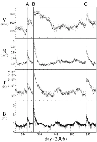
For these three events we show in Fig. 5 individual mea-surements of wind velocity, proton number density, and pro-ton temperature (at 4 or 8 min, depending on the spacecraft mode of operation), together with 1-m averages of the mag-netic field intensityB. The behaviour of these parameters strongly suggests that we are in the presence of shock-type events. A detailed analysis of the jumps in plasma and mag-netic parameters at A, B, and C has led to conclude that cases B and C satisfy all the required conditions to be classified as fast shocks, while for event A probably a shock structure is still under construction. Table 3 reports some of the com-puted parameters for events B and C. The shock normal is not far from the nominal Parker spiral (∼20◦ _{from radial).}

However, in both cases the upstream magnetic field is not close to its nominal orientation, with the result that its angle

αS with the shock normal is quite large.

In order to verify that the behaviour at lowτ of the S3 curve in Fig. 3 is essentially due to the variations at A, B, and C we have dropped some of the hourlyV data of the S3 sample (day 344 12–15, 345 5–15, and 351 17–22, cor-responding to the regions of magnetic field compression). In the top panel of Fig. 6 the rejected data are plotted in red. The new sample will be in the following indicated as S3∗

. The values ofδV0,δV1,δV2, andδV5 resulting from a new computation, based on S3∗

, of the velocity differences are shown in the four lower panels. It is easily seen that strong spikes as in Fig. 4 are no more observed. Thus, outliers in ve-locity differences are efficiently removed by eliminating just few velocity data points in connection with jumps at A, B, and C.

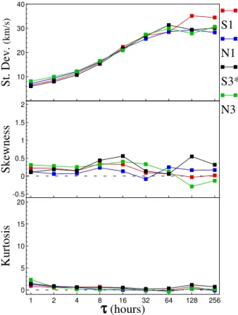
As a final check, in Fig. 7 the values of standard deviation, skewness, and kurtosis as obtained from the new sample S3∗

(black curves) are compared to those of samples S1, N1, and N3. It is easily seen that differences in skewness and kurto-sis have disappeared, and strong departures from a Gaussian behaviour are no more observed.

750 800 850

(km/s)

V

0.2 0.4 0.6 0.8 1

(cm

N

105

2*105

3*105

4*105

5*105

(K)

T

344 346 348 350 352

0 1 2 3

(nT)

day (2006)

B

A B

C

Fig. 5.From top to bottom: solar wind velocityV, proton number

densityN, proton temperatureT, and magnetic field magnitudeB

for the events A, B, and C shown in Fig. 4. The time resolution is 4 or 8 min for plasma data, depending on the spacecraft mode of operation, and 1 min for magnetic data.

4 Summary and conclusions

The out-of-ecliptic data set of Ulysses, covering about seven-teen years, allows to perform a comparison between proper-ties of the high-latitude heliosphere in consecutive solar cy-cles, hence for opposite polarity of the Sun’s magnetic field. In the present study we have looked at the behaviour of the solar wind velocity at high latitudes for low-activity phases of cycle 22 (1994–1996) and 23 (2006–2008) as observed by Ulysses during its first and third out-of-ecliptic orbit, respec-tively.

An overall view of the wind velocity distributions at lati-tudes above 40◦

–50◦

344 346 348 350 352 700

750 800 850

(2006)

(km/s)

day

V

-50 0 50

(km/s)

V0

=1h

-50 0 50

(km/s)

V1

=2h

-50 0 50

(km/s)

V2

=4h

320 340 360 15 35

-50 0 50

(2006)

(km/s)

day

V5

=32h

A B C

Fig. 6.The top panel shows, in an expanded time scale, the hourly

V values for an interval including events A, B, and C. Data

plot-ted in red have not been used in a new computation of the velocity

differencesδV n. The new values ofδV0,δV1,δV2, andδV5 are

given in the four lower panels.

rotation), with a regular increase in velocity for increasing latitude. In the Southern Hemisphere (panel South 1) this trend is less clear and variations between consecutive rota-tions may be relevant. For the third orbit, as already indi-cated by McComas et al. (2008), the velocity is appreciably lower than for the first orbit. However, the main belt of the distributions, representing the great majority of the velocity values, exhibits a shape similar to that of the first orbit sam-ples. At the same time the polar wind appears confined to higher latitudes.

The main goal of our study is that of characterizing the wind velocity variations at scales between 1 h and 10 days (or, more precisely, 256 h). With this choice we are looking at variations spanning from scales at which turbulence is known to develop up to scales at which conditions at the source so-lar region and propagation effects become relevant. Changes in power spectra across the investigated scales (Bavassano et al., 2005) are indicative of the different nature of the anal-ysed variations. The method used here to characterize wind velocity variations is that of a multi-scale statistical analysis of the velocity differences (see Burlaga and Forman, 2002). This kind of analysis has been done for samples at very

10 20 30 40

St.

Dev.

(km/s)

S1

N1

S3*

N3

-0.5 0 0.5 1 1.5 2

Skewness

1 2 4 8 16 32 64 128 256 0

5 10 15 20

(hours)

Kurtosis

Fig. 7.From top to bottom: standard deviation, skewness, and

kur-tosis versus time lagτ. The samples S1, N1, and N3 are the same

as in Fig. 3, while for the third orbit southern phase the sample S3∗

(derived from S3 by removing the data points shown in red in Fig. 6) is used.

high latitudes (three solar rotations at latitude above∼₇₀◦_), namely for solar wind flowing from central regions of the polar coronal hole.

Our results show that the structure of the velocity differ-ences between 1 h and several days essentially remains un-changed in different hemispheres and for different solar cy-cles (see Fig. 7). Thus, though the three-dimensional struc-ture of the heliosphere exhibits significant differences be-tween the first and third out-of-ecliptic orbit of Ulysses (Mc-Comas et al., 2006, 2008), at the investigated scales velocity variations appear to have very similar statistical properties in heliospheric regions at latitude above∼70◦_{. In}

It is noteworthy, however, that all this has been obtained after removal of few outliers in the data sample of the third orbit southern phase (S3). Three cases of sudden variation in the wind velocity were observed for this sample, noticeably affecting skewness and kurtosis at small scale. Two of these cases have been identified as fast forward shocks, while for the third case it can only be said that probably a shock struc-ture is still under construction. The observation of shocks at latitudes above 70◦

is not usual and indicates that also in central regions of the polar coronal hole the velocity inhomo-geneities may be large enough to build a shock discontinuity. The velocity microstructure is very probably related to the magnetic flux-tube texture of the solar wind (e.g., see Borovsky, 2008). Thus, our results could indicate that, in the core of polar coronal holes, such magnetic texture is an almost unchanging feature. This may affect relevant helio-spheric processes as, for instance, plasma turbulence and propagation of energetic particles. This conclusion, however, needs to be supported by further studies.

Acknowledgements. The use of data of the plasma analyser

(princi-pal investigator D. J. McComas, Southwest Research Institute, San Antonio, Texas, USA) and of the magnetometers (principal investi-gator A. Balogh, The Blackett Laboratory, Imperial College, Lon-don, UK) aboard the Ulysses spacecraft is gratefully acknowledged. The data have been made available through the World Data Center A for Rockets and Satellites (NASA/GSFC, Greenbelt, Maryland, USA). The present work has been supported by the Italian Space Agency (ASI) under contract I/035/05/0 ASI/INAF-OATO.

Topical Editor R. Forsyth thanks R. Skoug and another anony-mous referee for their help in evaluating this paper.

References

Bavassano, B., Bruno, R., and D’Amicis, R.: Large-scale velocity fluctuations in polar solar wind, Ann. Geophys., 23, 1025–1031, 2005, http://www.ann-geophys.net/23/1025/2005/.

Bavassano, B., D’Amicis, R., and Bruno, R.: Solar wind velocity at solar maximum: A search for latitudinal effects, Ann. Geophys., 22, 3721–3727, 2004,

http://www.ann-geophys.net/22/3721/2004/.

Borovsky, J. E.: Flux tube texture of the solar wind: Strands of the magnetic carpet at 1 AU?, J. Geophys. Res., 113, A08110, doi:10.1029/2007JA012684, 2008.

Burlaga, L. F. and Forman, M. A.: Large-scale speed fluctuations

at 1 AU on scales from 1 hour to≈1 year: 1999 and 1995, J.

Geophys. Res., 107, 1403, doi:10.1029/2002JA009271, 2002. Burlaga, L. F., Wang, C., Richardson, J. D., and Ness, N. F.:

Evolution of the multi-scale statistical properties of corotat-ing streams from 1 to 95 AU, J. Geophys. Res., 108, 1305, doi:10.1029/2003JA009841, 2003.

McComas, D. J., Barraclough, B. L., Funsten, H. O., Gosling, J. T., Santiago-Mu˜noz, E., Skoug, R. M., Goldstein, B. E., Neuge-bauer, M., Riley, P., and Balogh, A.: Solar wind observations over Ulysses first full polar orbit, J. Geophys. Res., 105, 10419– 10433, 2000.

McComas, D. J., Ebert, R. W., Elliott, H. A., Goldstein, B. E., Gosling, J. T., Schwadron, N. A., and Skoug, R. M.: Weaker solar wind from the polar coronal holes and the whole Sun, Geo-phys. Res. Lett., 35, L18103, doi:10.1029/2008GL034896, 2008. McComas, D. J., Elliot, H. A., Gosling, J. T., and Skoug, R. M.: Ulysses observations of very different heliospheric structure dur-ing the declindur-ing phase of solar acitivity cycle 23, Geophys. Res. Lett., 33, L09102, doi:10.1029/2006GL025915, 2006.

McComas, D. J., Elliott, H. A., Schwadron, N. A., Gosling, J. T., Skoug, R. M., and Goldstein, B. E.: The three-dimensional so-lar wind around soso-lar maximum, Geophys. Res. Lett., 30, 1517, doi:10.1029/2003GL017136, 2003.

Neugebauer, M.: The three-dimensional solar wind at solar activity minimum, Rev. Geophys., 37, 107–126, 1999.

Neugebauer, M., Gloeckler, G., Gosling, J. T., Rees, A., Skoug, R., Goldstein, B. E., Armstrong, T. P., Combi, M. R., M¨akinen, T., McComas, D. J., von Steiger, R., Zurbuchen, T. H., Smith, E. J., Geiss, J., and Lanzerotti, L. J.: Encounter of the Ulysses spacecraft with the ion tail of comet McNaught, Astrophys. J., 667, 1262–1266, 2007.