www.nonlin-processes-geophys.net/19/421/2012/ doi:10.5194/npg-19-421-2012
© Author(s) 2012. CC Attribution 3.0 License.
Nonlinear Processes
in Geophysics
Possible link between Holocene East Asian monsoon and solar
activity obtained from the EMD method
H. Y. Liu, Z. S. Lin, X. Z. Qi, Y. X. Li, M. T. Yu, H. Yang, and J. Shen
College of Geography Science, Nanjing Normal University, Nanjing, 210046, China
Correspondence to:Z. S. Lin ([email protected])
Received: 18 March 2010 – Revised: 6 July 2012 – Accepted: 10 July 2012 – Published: 10 August 2012
Abstract. It is thought that East Asian monsoon (EAM) is linked and sensitive to solar activity. In this paper, we have decomposed the Dongge cave speleothemδ18O record (proxy for EAM), and114C and10Be (proxies for solar ac-tivity) time series into variations at different time scales with the empirical mode decomposition (EMD) method to reveal the possible link between the EAM variability and solar ac-tivity. There are some common cycles in the EAM and solar variability from centennial to millennial scales, indicating a possible link between EAM and solar activity at these time scales. The correlation between EAM and solar activity is much higher at millennial scales than at centennial scales, which means direct responses to the solar variation are more likely at time scales longer than a few hundred years. At
∼30, 60 and 600 yr time scales, the variation in EAM is am-plified by the solar amplitude modulation at∼100, 200 and 2200 yr time scales.
1 Introduction
The Holocene has long been regarded as an analog to the future of natural environment process, which began at the end of the Pleistocene (around 12 000 yr BP) and continues to the present. Detailed studies of Holocene climate change and the controlling mechanisms can provide a context for present and future global change, and increase our under-standing of the underlying mechanisms of natural climate variability (Xue and Zhong, 2011). The East Asian mon-soon (EAM) is an integral part of the global climatic system, which regulates global atmospheric circulation through heat and moisture transport from the warmest part of the tropi-cal ocean, the west Pacific Warm Pool (WPWP), to higher latitudes (Wang et al., 2005), and plays a significant role
in the socio-economic life of people in East Asia (Zong et al., 2006). Increasing evidence shows that there were abrupt changes and periodic fluctuations in East Asian monsoon on decadal to millennial scales during the Holocene (Sirocko et al., 1993; Hong et al., 2000; Gupta et al., 2003; Fleit-mann et al., 2003). There are many factors affecting the East Asian monsoon, including orbitally induced insolation changes, changes in solar output, and changes in oceanic and atmospheric circulation (Wang et al., 2005). A number of existing high-resolution Holocene monsoon reconstruc-tions from Indian and Asian monsoon domains, and some modelling studies, reveal an influence of solar variation on East Asian monsoon (Joussaume et al., 1999; Neff et al., 2001; Fleitmann et al., 2003; Gupta et al., 2003; Wang et al., 2005), which can be explained by a direct solar influence on the Intertropical Convergence Zone (ITCZ) that controls the monsoonal precipitation (Kodera, 2004). Asian monsoon is thought to be sensitive to relatively small changes in solar forcing (0.25 % change in solar output) (Neff et al., 2001; Fleitmann et al., 2003). The mechanism is not very clear (Cosford et al., 2008). It is suggested to be amplified by the Pacific Decadal Oscillation and El Ni˜no-Southern Oscillation (ENSO) (Mann et al., 2005), and the North Atlantic Oscilla-tion (Gimeno et al., 2003) or be due to the threshold effects (Dykoski et al., 2005).
Most of the previous studies explored the possible link be-tween Asian monsoon and solar activity by direct compar-isons among different proxy records (Hu et al., 2003; Gupta et al., 2003) or by the presence of some periodicities and co-herence at certain bandwidths with respect to the 14C and 10Be data with spectral analysis (Dykoski et al., 2005; Xiao et al., 2006) and wavelet analysis (Witt and Schumann, 2005; Rousse et al., 2006; Cosford et al., 2008). Spectral analy-sis is a global analyanaly-sis that gives the frequency components
contained in the signal. It lacks the time localization of the spectral components. This type of analysis works best when the input signal is linear and stationary (Brigham, 1988; Qian, 2002). Short-time Fourier transform is able to capture the time-dependence of frequency fluctuations from nonsta-tionary data. However, in order to localize an event precisely in time, the window width must be narrow. Alternately, the frequency resolution requires longer time spans. This leads to conflicting requirements (Heisenberg-Gabor inequality) and restrains this method from many practical applications (Barnhart and Eichinger, 2011). The wavelet analysis has been applied to diagnose climate changes. It has good abil-ity to make multi-resolution analysis in both time domain and frequency domain. However, the choice of wavelet basis functions limits the applicability of the technique, as the ba-sic functions of wavelet transformation are fixed and do not necessarily match the shape of the considered data series in every instant in time (Torrence and Compo, 1998).
A relative new time-frequency analysis method, desig-nated empirical mode decomposition (EMD), has been pro-posed by Huang et al. (1998). The method essentially de-composes the original signal into a number of intrinsic mode function (IMF) components based on the local characteristic time scale of the signal and a residue. The EMD method is self-adaptive because the IMFs, working as the basis func-tions, are determined by the signal itself rather than what is pre-determined. Therefore, the EMD method is efficient in data analysis (Huang et al., 1998; Huang and Wu, 2007; Wu et al., 2007). In this paper, we will apply the EMD method to reveal the possible link between EAM and solar activity.
2 EMD method and data source
2.1 EMD method
According to the definition of the EMD method (Huang et al., 1998; Huang and Wu, 2007; Wu et al., 2007; Huang and Shen, 2005), the signal is decomposed into a finite num-ber of IMFs, each of which represents a simple oscillatory mode and satisfies the following two conditions to ensure there are no riding waves (i.e. the wave motion formed by small-scale perturbation waves superposed on long-scale un-perturbed waves): (1) in the whole dataset of the IMF, the number of extrema and the number of zero crossings must either be equal or differ at most by one; (2) at any point of the IMF, the mean value of the envelopes defined by the local maxima (relative maximum values that are greater than those values at the surrounding points), and local minima (relative minimum values that are smaller than those values at the sur-rounding points) is zero.
The decomposition method uses envelopes defined by the local maxima and the local minima of the original time series
X(t ), respectively. Firstly, all local extrema are identified, and then all local maxima are connected by a cubic spline to
form the upper envelope and minima are connected to form the lower envelope. Their mean is designated asm11(t ), and the difference betweenX(t )andm11(t )is the first compo-nent,h11(t ), i.e.
h11(t )=X(t )−m11(t ) . (1)
However,h11(t )is still not stationary. So, the above pro-cess is repeated.
h12(t )=h11(t )−m12(t ). (2)
m12(t )is the mean envelope ofh11(t ).
Further iterations of this sifting process proceed until a standard deviation (SD) criterion is met. The SD is typically set between 0.2–0.3 (Huang et al., 1998).
SD= T
X
t=0
"
(h1(i−1)(t )−h1i(t )
2
h21(i−1)(t ) #
(3)
T is the time length.
When SD criterion is satisfied afterkiterations, then
h1k(t )=h1(k−1)(t )−m1k(t ). (4)
The first IMF component (c1=h1k(t ))is separated from the
rest of the data by
r1=X(t )−c1. (5)
Sincer1still contains information of longer period compo-nents, it is treated as the new data and subjected to the same sifting process as described above. The process is repeated andri is described as follows:
r1=X(t )−c1, r2=r1−c2,· · ·, rn=rn−1−cn (6)
i.e.X(t )= n
X
i=1
ci+rn (7)
orX(t )= n
X
i=1
IMFi(t )+rn (8)
The sifting process can be stopped by any of the follow-ing predetermined criteria: either when the component,cn,
or the residue,rn, becomes so small that it is less than the
predetermined value of substantial consequence, or when the residue,rn, becomes a monotonic function from which no
more IMF can be extracted. Thus, we decomposeX(t )into
ci=IMFi(t )withi=1,2,3· · ·, nand a residue,rn, which
can be either the mean trend or a constant.
To illustrate how the EMD method works, we consider a 1000 s, three-frequency (f1=1/21, f2=1/41 and f3= 1/100 Hz) time series with Gaussian white noise (G(t )) as follows:
f (t )=1.5×eξ2πf1tcos(2πf
1t ) (9)
+1.5×e−ξ2πf2tcos(2πf
-10
0 10
S
ig
nal
-5 0 5
IM
F
1
-1 0 1
IM
F
2
-2 0 2
IM
F
3
-0.020 0.04
IM
F
4
100 200 300 400 500 600 700 800 900 1000 0
0.1 0.2
R
e
si
dual
Time[Second]
Fig. 1. Signal f (t )=1.5×eξ2πf1tcos(2πf
1t )+1.5×
e−ξ2πf2tcos(2πf
2t )+2×cos(2πf3t )+G(t ) and its
decom-positions using the EMD method. (f1=1/21, f2=1/41,
f3=1/100 Hz, ξ=0.01 and the standard deviation of the
mean-zero white noise is 10 % of the signal strength).
whereξ =0.01 and the standard deviation of the mean-zero white noise is 10 % of the signal strength.
The signal was decomposed into four IMF components and a residue with the EMD method (Fig. 1). The frequen-cies of the four IMF components are 1/21, 1/40.8, 1/99.7, and 1/280 Hz from high to low. The frequencies of IMF1, IMF2 and IMF3 are in good accord with the original three frequencies. The IMF4 and the residual may be mainly con-tributed by the Gaussian white noise. So, EMD method can decompose the original signal into a number of IMF com-ponents from high frequency to low frequency in order and adaptively.
Although the EMD method is powerful, one difficulty en-countered when using EMD is the influence of the end point treatment. The envelopes are calculated using a cubic spline. However, splines are notoriously sensitive to end points. It is important to make sure that the end effects do not propagate into the interior solution (Lin and Wang, 2006).
2.2 Data source
Speleothems can have continuous deposition of calcium carbonate over long periods of time, and well-chosen speleothems are datable with high precision. Absolute ages can be determined by means of230Th dating by mass spec-trometry (Dykoski et al., 2005; Cosford et al., 2008). Pre-vious studies have shown that shifts in the oxygen isotope ratio (δ18O) of the stalagmite from the cave largely reflect changes inδ18O values of meteoric precipitation at the site,
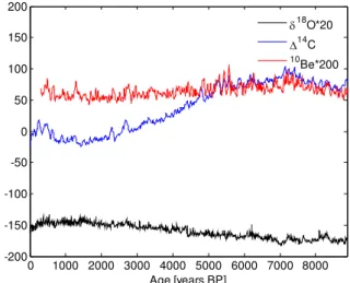
0 1000 2000 3000 4000 5000 6000 7000 8000 -200
-150 -100 -50 0 50 100 150 200
Age [years BP]
δ18
O*20
Δ14
C
10
Be*200
Fig. 2.Original signals ofδ18O,114C and10Be records.
which in turn relate to changes in the amount of precipitation and thus characterize the Asian monsoon strength (Dykoski et al., 2005).δ18O time series (from 9 ka BP to the present; the present is defined as the year 1950 AD) of stalagmite DA from Dongge cave, southern China, with an average temporal resolution of 4–5 yr are used as a proxy of the high-resolution absolute-dated Holocene Asian monsoon record (Wang et al., 2005). Chronology of the 962.5-mm-long stalagmite DA is established by 45230Th dates, all in stratigraphic order, with a typical age uncertainty of 50 yr (Wang et al., 2005).
Owing to the lack of complete direct observations of the Sun for the period before 1600 AD, cosmogenic radionu-clides 14C (recorded in tree rings) and 10Be (preserved in polar ice cores) are used as indirect proxies of solar vari-ability (Yiou et al., 1997; Stuiver et al., 1998; Wagner et al., 2001; Muscheler et al., 2007). During the periods of lower sunspot activity, solar wind intensity is reduced, which in-creases the influx of galactic cosmic rays. A higher influx of cosmic rays increases the production of14C and10Be in the atmosphere. The reverse is true during the periods of increased sunspot activity when less14C and 10Be are pro-duced. Therefore, changes in atmospheric 114C and 10Be can be related to changes in solar activity. In this paper, the tree-ring 114C record (from 9000 yr BP to the present) is from the IntCal04 calibration curve with 1-standard devia-tion envelope and data with 1-standard deviadevia-tion error bars in14C and calibrated age (Reimer et al., 2004) .The 10Be record (from 304 to 9315 yr BP) is from Greenland Ice Core Project (GRIP) ice core (Yiou et al., 1997; Wagner et al., 2001; Muscheler et al., 2007) with 5 yr temporal resolutions, and we use the timescale published by Johnsen et al. (1997) (ss09 timescale) by counting annual layers in the GRIP core. The datasets ofδ18O,114C and10Be spaced at 10 yr in-tervals (Fig. 2) are decomposed into signals at different time scales for further comparisons with the EMD method to
reveal the possible link between solar activity and EAM in-tensity on different time scales.
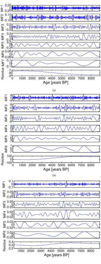
3 EMD analysis ofδ18O,114C and10Be
The EMD method was utilized to extract the intrinsic cycles of the datasets ofδ18O, 114C and 10Be (Fig. 3). The time series ofδ18O was decomposed into seven IMF components and a residue, and the time series of10Be and 114C were decomposed into six IMF components and a residue respec-tively. The cycle of each IMF component is calculated using zero-crossing method.
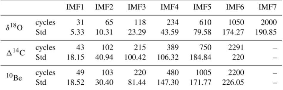
The IMF components of δ18O correspond to decadal to millennial scale cycles centering on 31, 65, 118, 234, 600, 1050 and 2000 yr (Table 1), which are close to the cycles of 2040, 930, 568, 212, 120, 65 and 28 yr in spectral analy-sis (Fig. 4a). In spectral analyanaly-sis, centennial to multi-millennial cycles are stronger than multi-decadal cycles.
The cycles of the IMF components of114C centre on 43, 102, 215, 389, 750, 2291 yr. The cycles of 102, 215, 389 and 2291 yr are close to 104, 207, 350 and 2400 yr, which are strong in spectral analysis (Fig. 4b). These cycles are also revealed by previous studies (Stuiver and Braziunas, 1993; Ogurtsov et al., 2002). Although∼750 and 2291 yr are not
observed in the spectral analysis,∼750 yr cycle is reported
in another study (Clemens, 2005), and ∼2291 yr cycle is
close to the Hallstatt cycle, which is revealed by Miller and Scott (1995) and Usoskin et al. (2009).
The cycles of the IMF components of10Be centre on 49, 103, 220, 480, 1005 and 2200 yr, which is similar to the re-sults of Yin et al. (2007). Cycles of 49, 103, 220 and 1005 yr are also revealed in spectral analysis (Fig. 4c).
By the comparison of solar activity reconstructions from 10Be GISP series and from 114C series, Vonmoos et al. (2006) have shown that the agreement between them is good on centennial to millennial timescale. With the EMD method, the records of 114C and 10Be also show concur-rent cycles on∼100, 200, 1000 and 2200 yr. The correlation
coefficients on these scales are higher than on multi-decadal scales (Table 2). Although the cycle of IMF1 of114C (44 yr) is close to that of10Be (49 yr), the correlation coefficient is very low (Table 2). Herein, good agreement between114C and10Be on centennial to millennial timescale implies that the variations at these cycles are more likely caused by the solar modulation than at multi-decadal scales.
Although114C and10Be are both used as proxy of solar activity, there are some discrepancies in their cycles. The cy-cle of IMF4 of114C is 389 yr, while that of10Be is 480 yr. The 389 yr cycle is close to a 360 yr tidal cycle (Keeling and Whorf, 2000), and observed in a high-resolutionδ18O record of peat cellulose in the Jilin Province in China (Hong et al., 2000), and in slope sediments of the Great Bahama Bank (Roth and Reijmer, 2005).The worldwide appearance of this signal thus points to the involvement of oceanic and
-0.250 0.25 IM F 1 -0.150 0.15 IMF 2 -0.20 0.2 IM F 3 -0.20 0.2 IMF 4 -0.20 0.2 IM F 5 -0.080 0.08 IM F 6 -0.10 0.1 IMF 7
0 1000 2000 3000 4000 5000 6000 7000 8000 -9 -8 -7 R es idue
Age [years BP]
(a) -40 4 IMF 1 -8 0 8 IM F 2 -80 8 IM F 3 -40 4 IM F 4 -70 7 IM F 5 -70 7 IMF 6
0 1000 2000 3000 4000 5000 6000 7000 8000 -100 0 100 R e si due
Age [years BP]
(b) -0.1 0 0.1 IM F 1 -0.050 0.05 IMF 2 -0.050 0.05 IM F 3 -0.020 0.02 IMF 4 -0.020 0.02 IM F 5 -0.020 0.02 IM F 6
1000 2000 3000 4000 5000 6000 7000 8000 0.2 0.3 0.4 Re s id u e
Age [years BP]
(c)
Fig. 3.EMD analysis ofδ18O(a),114C(b)and10Be(c)records.
Table 1.Cycles ofδ18O,114C and10Be with the EMD method.
IMF1 IMF2 IMF3 IMF4 IMF5 IMF6 IMF7
δ18O cycles 31 65 118 234 610 1050 2000 Std 5.33 10.31 23.29 43.59 79.58 174.27 190.85
114C cycles 43 102 215 389 750 2291 – Std 18.15 40.94 100.42 106.32 184.84 220 –
10Be cycles 49 103 220 480 1005 2200 –
Std 18.52 30.40 81.44 147.30 171.77 226.05 –
Table 2. Correlation coefficients(r)of IMFs between 114C and
10Be.
Signal IMF1 IMF2 IMF3 IMF4 IMF5 IMF6
0.6 0.0721 0.2305 0.4833 0.2447 0.5941 0.824
large-scale atmospheric processes causing cyclicities with this frequency (Roth and Reijmer, 2005).The∼500 yr oscil-lation is thought to reflect a climatic process, involving ther-mohaline circulation and atmospheric processes that influ-enced atmospheric and oceanographic dynamics (Roth and Reijmer, 2005). Moreover, this cycle is possible to be a har-monic of the reported millennial-scale cycles or a subhar-monic of the reported century-scale cycles.
Previous studies have pointed out that the short-term variations in 10Be are mainly controlled by local climate (Muscheler et al., 2007; Usoskin et al., 2009). The EMD analysis shows that the amplitudes of10Be variation at short time scales are larger than those at long time scales (Fig. 3c). Moreover, the spectral analysis reveals there are many mul-tidecadal cycles in10Be record (Fig. 4c). So, local climate may dominate the10Be data on short timescales as Usoskin et al. (2009) pointed out. Conversely, the amplitudes of short-time variation in114C are smaller than those of long-term variation (Fig. 3b), which is suggested to be due to the am-plification of carbon cycle at long time scales by Muscheler et al. (2007).
4 Relations between solar variability and East Asian monsoon at different time scales
Most of the cycles found in Sect. 3 have been reported from mid to high northern latitudes (Bond et al., 2001; Hu et al., 2003) to low-latitude regimes (Fleitmann et al., 2003), in-cluding the Asian monsoon region (Wang et al., 2005; Xiao et al., 2006; Thamban et al., 2007). The cycles of ∼118, 234, 1050 and 2000 yr closely match those of 114C and 10Be. ∼118 and 234 yr cycles are close to 90 yr (Gleiss-berg) and 207 yr (Suess) solar cycles. The century-type cy-cle of Gleissberg has a wide frequency band with a double
structure consisting of 50–80 yr and 90–140 yr periodicities, and the Suess cycle is less complex showing a variation with a period of 170–260 yr (Ogurtsov et al., 2002). These two cy-cles have been reported from East Asian monsoon (Dykoski et al., 2005; Xiao et al.,2006; Cosford et al., 2008), Indian monsoon (Neff et al., 2001; Agnihotri et al., 2002; Fleitmann et al., 2003; Thamban et al., 2007) and American monsoon (Asmerom et al., 2007; Str´ıkis et al., 2011) based on a variety of climate proxies. The ∼1000 yr cycle is widely reported in stalagmites from Oman (Neff et al., 2001), sediments of the Arabian Sea (Thamban et al., 2007), peat cellulose from Hongyuan and Jinchuan (Xu et al., 2002) and lake sediments from Alaska (Hu et al., 2003). Its global nature due to the hemisphere-wide presence of this periodicity (Thamban et al., 2007) and its presence in10Be data support that it is re-lated to the variations in solar activity. The∼2000 yr cycle
was recorded in sediments of the Arabian Sea (Thamban et al., 2007) and Yangtze River-derived mud in the East China Sea (Xiao et al., 2006). The cycle was close to the 2560 yr recorded in the Camp Century ice coreδ18O profile (Dans-gaard et al., 1984) and in the Okinawa Trough (Jian et al., 2000). The114C and10Be records both reveal∼2200 yr cy-cle, which is also revealed by other studies (Stuiver and Braz-iunas, 1993; Lean, 2002) and is close to Hallstattzeit cycle. Hence, ∼2200 yr cycle may be linked to solar variability. Moreover, oceanic circulation is thought to play a significant role in transferring and modulating the variability at this time scale (Naidu and Malmgren, 1995; Thamban et al., 2007).
Although common cycles on ∼100, 200, 1000 and 2000 yr do not necessarily suggest a mechanistic link, they do indicate a possible link between the EAM and solar activ-ity. As shown from Table 3, at millennial scales (∼1000 and
2000 yr), the correlations between EAM and solar activity are much higher than at centennial scales, which means solar activity has greater influences on EAM at millennial scales.
The∼30 and 60 yr cycles are very common in not only the modern but also secular monsoon records, including East Asian monsoon and India monsoon (Minobe, 1997; Agni-hotri et al., 2002; Clemens, 2005; Dykoski et al., 2005; Wang et al., 2005; Mazzarella and Scafetta, 2012). However, both
114C and10Be records do not reveal these two cycles with the EMD method. It seems there is no direct relation between
0 0.01 0.02 0.03 0.04 0.05
0 1 2 3 4 5 6 7 8
Frequency [year-1]
S
pect
ral
A
m
pl
it
ude
2040
930
568
43
28 23
153 212
120 65 88
(a)
0 0.005 0.01 0.015 0.02
0 0.5 1 1.5 2 2.5 3 3.5
4x 10 4
Frequency [year-1]
S
pect
ral
A
m
pl
it
ude
231
207 149 130 104 88 350
2400
950
560
(b)
0 0.01 0.02 0.03 0.04 0.05
0.05 0.1 0.15 0.2 0.25 0.3 0.35 0.4 0.45 0.5 0.55
Frequency [year-1]
S
pect
ral
A
m
pl
it
ude
146 208
66 55
46 356
130 105
87 950
(c)
Fig. 4.Power spectrum using REDFIT3.6 (Schulz and Mudelsee, 2002) forδ18O(a), 114C(b)and 10Be(c)records. Default pa-rameters are used except that the parameter ofn50 representing the Welch’s overlap segment averaging is 4 and Welch spectrum win-dow is chosen (refer to Schulz and Mudelsee, 2002 for details).
0 1000 2000 3000 4000 5000 6000 7000 8000 9000
-100 -50 0 50 100 150 200 250 300
Age [years BP]
Residue of δ18O*10
Residue of Δ14C
Residue of 10Be*500
Fig. 5.Residues ofδ18O(a),114C(b)and10Be(c)records.
solar variability and EAM variation at multi-decadal time scales. However, the atmospheric pressure changes associ-ated with the North Atlantic Ocean (NAO), and changes in sea-surface temperatures and thermohaline circulation as-sociated with the Atlantic Multidecadal Oscillation (AMO) exhibit a ∼60 yr cycle (Schlesinger and Ramakutty, 1994;
Kerr, 2000; Gimeno et al., 2003; Knudsen et al., 2011). Moreover, the Pacific Decadal Oscillation (PDO) resembles the well-known ENSO system, but operates in the North Pacific and exhibits 25–35 yr and 50–70 yr cycles (Minobe, 1997). So,∼30 and 60 yr cycles are thought to be linked to
the Pacific Decadal Oscillation and the North Atlantic Os-cillation (Schlesinger and Ramankuty, 1994; Gimeno et al., 2003; Knudsen et al., 2011; Mazzarella and Scafetta, 2012).
∼600 yr cycle is revealed in the Lianhua A1, Heshang HS4, Dongge DA and D4 speleothemδ18O records (Cosford et al., 2008). It is close to the prominent 649 yr cycle discovered by Damon and Sonett (1991) and is thought to be related to so-lar variability (Zhu et al., 2009). However, this cycle is not observed in114C and10Be records with the EMD method. Hence, it seems that solar variability has few or indirect in-fluence on EAM at this time scale.
The residues ofδ18O,114C and10Be have been compared to show their long-term trends (Fig. 5). The residue ofδ18O increased gradually, which means the Asian monsoon weak-ened through the Holocene. It is thought to be caused by the gradual decrease in summer insolation (Overpeck et al., 1996). The long-term trend ofδ18O is quite different from that of114C and 10Be, which means that different driving forces control them. It is because the radionuclide production rates on long time scales (>3000 yr) are probably caused by geomagnetic modulation and those on short time scales (<3000 yr) are most likely of solar origin (Beer, 2000).There is a slight discrepancy between the long-term trend of114C and10Be. Whether this discrepancy is mainly due to changes in the114C or the10Be system cannot yet be decided without further information (Vonmoos et al., 2006; Muscheler et al., 2007).
Table 3.Correlation coefficients (r)δ18O with114C and10Be at
∼100, 200, 1000 and 2000-yr time scales.
δ18O Correlation ∼100 ∼200 ∼1000 ∼2000 coefficients (r)
114C 0.23 −0.0161 0.2944 −0.5551
10Be 0.1145 0.2385 0.4298 −0.6096
5 Possible solar modulation of East Asian monsoon
Both radionuclides exhibit the same solar signal despite the fact that different conditions influenced their concen-trations before their deposition in the archives (Vonmoos et al., 2006). However, 10Be has a better correlation with
δ18O than114C (Table 3). Especially, at∼200 yr time scale, correlation coefficient between114C andδ18O is very low (r= −0.0161), while that between10Be andδ18O is remark-able (r=0.2385). It seems that there is almost no correlation between114C andδ18O at this time scale. Therefore,10Be is used as a proxy of solar activity for further comparison with
δ18O in this article.
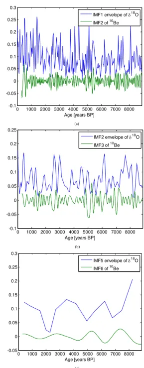
∼30, 60 and 600 yr cycles are absent in10Be and114C records with the EMD method. Although these cycles are observed in the spectral analysis in other studies (Neff et al., 2001; Fleitmann et al., 2003), they are too small to cause sig-nificant impact on the climate of the Earth. So, these three time scales are thought to be indirectly affected by solar variability through the interaction between atmospheric and ocean circulation that amplify this initial signal (Neff et al., 2001). With the EMD method, the amplitudes of these three IMFs of EAM change with time and, in fact, have charac-teristics of slowly varying wavelet packets (Fig. 4). So, there are possible amplitude modulations of EAM by some driv-ing forces at these time scales. The envelope of an IMF is symmetric, so it is only necessary to examine the maximum values in order to identify the characteristics of this cycle (Lin and Wang, 2003). To reveal possible solar modulation of EAM, the envelopes of IMF1, IMF2 and IMF5 ofδ18O have been compared with IMF2, IMF3 and IMF6 of10Be respec-tively (Fig. 6). The crests of the envelope of the IMF1 ofδ18O largely coincide with the troughs of the IMF2 of10Be and vice versa (Fig. 6a), which means there is an inverse phase relation between them. Similarly, the envelopes of IMF2 and IMF5 ofδ18O are also in inverse phase with the IMF3 and IMF6 of 10Be in great part. So, ∼100, 200, 2000 yr solar variability are adaptations to∼30, 60 and 600 yr EAM vari-ation, and EAM variation is amplitude modulated by solar variation.
The∼200 yr Suess cycle and 2200 yr Hallstattzeit cycle are thought to modulate the century-type cycle of Gleiss-berg, and the century-type cycle of Gleissberg is thought to modulate the 11 yr Schwabe cycle (Peristykh and Damon, 2003). In this article,∼100, 200 and 2200 yr solar variations
0 1000 2000 3000 4000 5000 6000 7000 8000 -0.1
-0.05 0 0.05 0.1 0.15 0.2 0.25 0.3
Age [years BP]
IMF1 envelope of δ18
O
IMF2 of 10Be
(a)
0 1000 2000 3000 4000 5000 6000 7000 8000 -0.1
-0.05 0 0.05 0.1 0.15 0.2 0.25
Age [years BP]
IMF2 envelope of δ18O
IMF3 of 10Be
(b)
0 1000 2000 3000 4000 5000 6000 7000 8000 -0.05
0 0.05 0.1 0.15 0.2 0.25 0.3
Age [years BP]
IMF5 envelope of δ18O
IMF6 of 10Be
(c)
Fig. 6.Comparisons between the envelopes of IMFs ofδ18O and IMFs of 10Be. (a)IMF1 envelope of δ18O and IMF2 of 10Be.
(b)IMF2 envelope of 1δ18O and IMF3 of10Be.(c)IMF5 envelope ofδ18O and IMF6 of10Be.
are also thought to modulate EAM variations at ∼30, 60 and 600 yr, respectively. Moreover, solar variations at∼100, 200, 2000 yr time scales are as large as at the other time scales in both spectral and EMD analysis. So, the changes in solar variation at these three time scales may amplify the changes in EAM at 30, 60 and 600 yr time scales. By this way, small changes in solar activity at 30, 60 and 600 yr may
be able to trigger larger changes in EAM. Therefore, solar variability may be a plausible direct driver of EAM at these three time scales.
6 Conclusions
EAM and solar activity share some common cycles on
∼100, 200, 1000 and 2000 yr time scales. This supports the idea that solar changes are partly responsible for changes in Holocene EAM intensity from centennial to millennial scales (Dykoski et al., 2005; Wang et al., 2005; Cosford et al., 2008). Moreover, EAM and solar activity have much higher correlation at millennial time scales than at centennial time scales. This result also supports the assumption that a di-rect response to the solar variation holds more likely for time scales longer than a few hundred years (Weber et al., 2004).
The10Be and114C records do not reveal cycles at∼30, 60 and 600 yr, and, hence, it seems that there is no direct relation between EAM and solar activity at these time scales. How-ever, EAM intensity at these time scales is amplitude modu-lated by solar activities at∼100, 220, and 2200 yr, which im-plies that solar activity is a plausible driver of EAM at these time scales. So, EAM variation at∼30, 60 and 600 yr time scales may be directly amplified by solar activity. It may be a possible mechanism to explain why small changes in solar output at these time scales can cause large changes in EAM.
Acknowledgements. This research has been supported by China
NSF (No. 41173093, 40901094, 41030751), and funded by the Priority Academic Program Development of Jiangsu Higher Education Institutions and Jiangsu Oversea Research and Training Program for University Prominent Young and Middle-aged teachers and Presidents. We also thank the anonymous reviewers for helpful suggestions.
Edited by: J. Kurths
Reviewed by: two anonymous referees
References
Agnihotri, R., Dutta, K., Bhushan, R., and Somayajulu, B.: Evi-dence for solar forcing on the Indian monsoon during the last millennium, Earth. Planet. Sci. Lett., 198, 521–527, 2002. Asmerom, Y., Polyak, V., Burns, S., and Rasmussen, J.: Solar
forc-ing of Holocene climate: New insights from a speleothem record, southwestern United States, Geology, 35, 1–4, 2007.
Barnhart, B. L. and Eichinger, W. E.: Empirical Mode Decomposi-tion Applied to Solar Irradiance, Global Temperature, Sunspot Number, and CO2 Concentration Data, J. Atmos. Solar. Terr.
Phys., 73, 1771–1779, 2011.
Beer, J.: Long-term indirect indices of solar variability, Space. Sci. Rev., 94, 53–66, 2000.
Bond, G., Kromer, B., Beer, J., Muscheler, R., Evans, M. N., Show-ers, W., Hoffmann, S., Lotti-Bond, R., Hajdas, I., and Bonani,
G.: Persistent solar influence on North Atlantic Climate during the Holocene, Science, 294, 30–36, 2001.
Brigham, E.: The Fast Fourier Transform and its Applications, Pren-tice Hall, Englewood Cliffs, NJ, 1988.
Cosford, J., Qing, H., Eglington, B., Yuan, D. X., Zhang, M. L., and Chen, H.: East Asian monsoon variability since the Mid-Holocene recorded in a high-resolution, absolute-dated aragonite speleothem from eastern China, Earth. Planet. Sci. Lett., 275, 296–307, 2008.
Clemens, S. C.: Millennial-band climate spectrum resolved and linked to centennial-scale solar cycles, Quaternary Sci. Rev., 24, 521–531, 2005.
Damon, P. E. and Sonett, C. P.: Solar and terrestrial components of the atmospheric14C variation spectrum, in: The Sun in Time, edited by: Sonett, C. P., Giampapa, M. S., and Matthews, M. S., Univ. of Ariz. Press, Tucson, 360–388, 1991.
Dansgaard, W., Johnsen, S. J., Clausen, H. B., Dahl-Jensen, N., Gundestrup, N., and Hammer, C. U.: North Atlantic climatic os-cillations revealed by deep Greenland ice cores, in Climate Pro-cesses and Climate Sensitivity, Geophys. Monogr. Ser., 29, 288– 298, 1984.
Dykoski, C. A., Edwardsa, R. L., Cheng, H., Yuan, D. X., Cai, Y. J., Zhang, M. L., Lin, Y. S., Qin, J. M., and An, Z. S.: A high res-olution, absolute-dated Holocene and deglacial Asian monsoon record from Dongge Cave, China, Earth. Planet. Sci. Lett., 233, 71–86, 2005.
Fleitmann, D., Burns, S. J., Mudelsee, M., Neff, U., Kramers, J., Mangini, A., and Matter, A.: Holocene forcing of the Indian monsoon recorded in a stalagmite from Southern Oman, Science, 300, 1737–1739, 2003.
Gupta, A. K., Anderson, D. M., and Overpeck, J. T.: Abrupt changes in the Asian southwest monsoon during the Holocene and their links to the North Atlantic Ocean, Science, 42, 354–357, 2003. Gimeno, L., de la Torre, L., Nieto, R., Garcia, R., Hernandez, E.,
and Ribera, P.: Changes in the relationship NAO-Northern Hemi-sphere temperature due to solar activity, Earth. Planet. Sci. Lett., 206, 15–20, 2003.
Hu, F. S., Kaufman, D., Yoneji, S., Nelson, D., Shemesh, A., Huang, Y., Tian, J., Bond, G., Clegg, B., and Brown, T.: Cyclic variation and solar forcing of Holocene climate in the Alaskan subarctic, Science, 301, 1890–1893, 2003.
Huang, N. E., Shen, Z., and Long, S. R.: The empirical mode de-composition and the Hilbert spectrum for nonlinear and non-stationary time series analysis, Proc. R. Soc. Land. A., 454, 899– 955, 1998.
Huang, N. E. and Wu, Z.: A review on hilbert-huang transform: method and its applications to geophysical studies, Rev. Geo-phys., 46, RG2006, doi:10.1029/2007RG000228, 2007. Huang, N. E. and Shen, S. L.: Hilbert-Huang transform and its
ap-plications, World Scientific Press, Singapore, 2005.
Hong, Y. T., Jiang, H. B., Liu, T. S., Zhou, L. P., Beer, J., Li, H. D., Leng, X. T., Hong, B., and Qin, X. G.: Response of climate to so-lar forcing recorded in a 6000-yearδ18O time-series of Chinese peat cellulose, The Holocene, 10, 1–7, 2000.
Johnsen, S. J., Clausen, H. B., Dansgaard, W., Gundestrup, N. S., Hammer, C. U., Andersen, U., Andersen, K. K., Hvidberg, C. S., Dahl-Jensen, D., Steffensen, J. P., Shoji, H., Sveinbj¨ornsd´ottir,
´
A. E., White, J., Jouzel, J., and Fishe, D.: Theδ18O record along the Greenland Ice Core Project deep ice core and the problem of possible Eemian climatic instability, J. Geophys. Res., 102, 26397–26410, 1997.
Joussaume, S., Taylor, K. E., Braconnot, P., Webb, R. S., and Wy-putta, U.: Monsoon changes for 6000 years ago: results of 18 simulations from the Paleoclimate Modeling Intercomparison Project (PMIP), Geophys. Res. Lett., 26, 859–862, 1999. Keeling, C. D. and Wharf, T. P.: The 1800-year oceanic tidal cycle:
a possible cause of rapid climate change, Proc. Natl. Acad. Sci. USA, 97, 3814–3819, 2000.
Kerr, R. A.: A North Atlantic climate pacemaker for the centuries, Science, 288, 1984–1986, 2000.
Knudsen, M. F., Seidenkrantz, M., Jacobsen, B. H., and Kuijpers, A.: Tracking the Atlantic Multidecadal Oscilla-tion through the last 8,000 years, Nat. Commun., 2, 178, doi:10.1038/ncomms1186, 2011.
Kodera, K.: Solar influence on the Indian Ocean monsoon through dynamical processes, Geophys. Res. Lett., 31, L24209, doi:10.1029/2004GL020928, 2004.
Lin, Z. S. and Wang, S. G.: EMD Analysis of Solar Insolation, Me-teorol. Atmos. Phys., 93, 1871–1893, 2006.
Lean, J.: Solar forcing of climate change in recent millennia, in: Climate development and history of the North Atlantic realm, edited by: Wefer, G., Berger, W. H., Behre, K.-E., and Jansen, E., Berlin, Springer-Verlag, 75–88, 2002.
Mann, M. E., Cane, M. A., Zebiak, S. E., and Clement, A.: Volcanic and solar forcing of the tropical Pacific over the past 1000 years, J. Climate, 18, 447–456, 2005.
Mazzarella, A. and Scafetta, N.: Evidences for a quasi 60-year North Atlantic Oscillation, Theor. Appl. Climatol., 107, 599– 609, 2012.
Miller, B. F. and Scott, E. M.: Cosmogenic radiocarbon and cyclical natural processes, Radiocarbon, 37, 417–424, 1995.
Minobe, S.: A 50-70 year climatic oscillation over the North Pacific and North America, Geophys. Res. Lett., 24, 683–686, 1997. Muscheler, R., Joos, F., Beer, J., M¨uller, S. A., Vonmoos, M.,
and Snowball, I.: Solar activity during the last 1000 years in-ferred from radionuclide records, Quaternary Sci. Rev., 26, 82– 97, 2007.
Naidu, P. D. and Malmgren, B. A.: A 2200–2400 year periodicity in the Asian monsoon system, Geophys. Res. Lett., 22, 2361–2364, 1995.
Neff, U., Burns, S. J., Mangini, A., Mudelsee, M., Fleitmann, D., and Matter, A.: Strong coherence between solar variability and the monsoon, Nature, 411, 290–293, 2001.
Ogurtsov, M. G., Nagovitsyn, Y. A., Kocharov, G. E., and Jungner, H.: Long-period cycles of the Sun’s activity recorded in direct solar data and proxies, Sol. Phys., 211, 371–394, 2002. Overpeck, J., Anderson, D. M., Trumbore, S., and Prell, W.: The
southwest Indian Monsoon over the last 18,000 years, Clim. Dy-nam., 12, 213–225, 1996.
Peristykh, A. N. and Damon, P. E.: Persistence of the Gleiss-berg 88-yr solar cycle over the last 12,000 years: Evi-dence from cosmogenic isotopes, J. Geophys., 108, 1003, doi:10.1029/2002JA009390, 2003.
Qian, S.: Introduction to Time-Frequency and Wavelet Transforms, Prentice- Hall Inc., Upper Saddle River, NJ, 2002.
Reimer, P. J., Baillie, M. G. L., Bard, E., Bayliss, A., Beck, J. W., Bertrand, C. J. H., Blackwell, P. G., Buck, C. E., Burr, G. S., Cutler, K. B., Damon, P. E., Edwards, R. L., Fairbanks, R. G., Friedrich, M., Guilderson, T. P., Hogg, A. G., Hughen, K. A., Kromer, B., McCormac, G., Manning, S., Ramsey, C. B., Reimer, R. W., Remmele, S., Southon, J. R., Stuiver, M., Talamo, S., Tay-lor, F. W., van der Plicht, J., and Weyhenmeyer C. E.: IntCal04 terrestrial radiocarbon age calibration, 0–26 cal kyr BP, Radio-carbon, 46, 1029–1058, 2004.
Roth, S. and Reijmer, J. J. G.: Holocene millennial to centennial car-bonate cyclicity recorded in slope sediments of the Great Bahama Bank and its climatic implications, Sedimentology, 52, 161–181, 2005.
Rousse, S., Kissel, C., Laj, C., Eir´ıksson, J., and Knudsen, K. L.: Holocene Centennial to Millennial-scale climatic variability: ev-idence from high-resolution magnetic analyses of the last 10 cal kyr off North Iceland (core MD99-2275), Earth. Planet. Sci. Lett., 242, 390–405, 2006.
Schlesinger, M. E. and Ramakutty, N.: An oscillation in the global climate system of period 65–70 years, Nature, 367, 723–726, 1994.
Schulz, M. and Mudelsee, M.: REDFIT: Estimating red-noise spec-tra directly from unevenly spaced paleoclimatic time series, Comput. Geosci., 28, 421–426, 2002.
Sirocko, F., Sarnthein, M., Erlenkeuser, H., Lange, H., Arnold, M., and Duplessy, J. C.: Century-scale events in monsoonal climate over the past 24 000 years, Nature, 364, 322–324, 1993. Str´ıkis, N. M., Francisco, W., Cruz, F. W., Cheng, H., Karmann, I.,
Edwards, R. L., Vuille, M., Wang, F., de Paula, M. S., Novello, V. F., and Auler, A. S.: Abrupt variations in South American mon-soon rainfall during the Holocene based on a speleothem record from central-eastern Brazil, Geology, 39, 1075–1078, 2011. Stuiver, M., Reimer, P. J., Bard, E., Warreneck, J., Burr, G. S.,
Hughen, K. A., Kromer, B., McCormac, G., van der Plicht, J., and Spurk, M.: Intcal98 radiocarbon age calibration, 24000-0 cal BP, Radiocarbon, 40, 1041–1083, 1998.
Stuiver, M. and Braziunas, T. F.: Modeling atmospheric14C influ-ences and14C ages of marine samples to 10,000 BC, Radiocar-bon, 35, 137–189, 1993.
Thamban, M., Kawhata, H., and Rao, V. P.: Indian summer mon-soon variability during the Holocene as recorded in sediments of the Arabian Sea: Timing and implications, J. Oceanography, 63, 1009–1020, 2007.
Torrence, C. and Compo, G. P.: A practical guide to wavelet analy-sis, Bull. Am. Meteorol. Soc., 79, 61–78, 1998.
Usoskin, I. G., Horiuchi, K., Solanki, S., Kovaltsov, G. A., and Bard, E. : On the common solar signal in different cos-mogenic isotope data sets, J. Geophys. Res., 114, A03112, doi:10.1029/2008JA013888, 2009.
Vonmoos, M., Beer, J., and Muscheler, R.: Large variations in Holocene solar activity: Constraints from 10Be in the Green-land Ice Core Project ice core, J. Geophys. Res., 111, A10105, doi:10.1029/2005JA011500, 2006.
Wagner, G., Beer, J., Masarik, J., Muscheler, R., Kubik, P., Mende, W., Laj, C., Raisbeck, G. M., and Yiou, F.: Presence of the solar de Vries cycle (∼205 years) during the last ice age, Geophys. Res. Lett., 28, 303–306, 2001.
Wang, Y., Cheng, H., Edwards, L.R., He, Y., Kong, X., An, Z., Wu, J., Kelly, M. J., Dykoski, C. A., and Li, X.: The Holocene Asian monsoon: links to solar changes and north Atlantic climate, Sci-ence, 308, 854–857, 2005.
Weber, S. L., Crowley, T. J., and van der Schrier, G.: Solar irradiance forcing of centennial climate variability during the Holocene, Clim. Dynam., 22, 539–553, 2004.
Witt, A. and Schumann, A. Y.: Holocene climate variability on mil-lennial scales recorded in Greenland ice cores, Nonlin. Processes Geophys., 12, 345–352, 2005,
http://www.nonlin-processes-geophys.net/12/345/2005/. Wu, Z., Huang, N. E., Long, S. R., and Peng, C. K.: On the trend,
detrending, and variability of nonlinear and nonstationary time series, Proc. Natl. Aca. Sci., 104, 14889–14894, 2007.
Xiao, S. B., Li, A. C., Liu, P., Chen, M. H., Xi, Q., Jiang, F., Li, T. G., Xiang, R., and Chen, Z.: Coherence between solar activity and the East Asian winter monsoon variability in the past 8000 years from Yangtze River-derived mud in the East China Sea, Palaeogeogr. Palaeoclimatol., 237, 293–304, 2006.
Xu, H., Hong, Y., Lin, Q., Hong, B., Jiang, H., and Zhu, Y.: Temper-ature variations in the past 6000 years inferred fromδ18O of peat cellulose from Hongyuan, China, Chinese Sci. Bull., 47, 1578– 1584, 2002.
Xue, J. and Zhong, W.: Holocene climate variation denoted by Barkol Lake sediments in northeastern Xinjiang and its possi-ble linkage to the high and low latitude climates, Sci. China Ser. D-Earth Sci., 54, 603–614, 2011.
Yiou, F., Raisbeck, G. M., Baumgartner, S., Beer, J., Hammer, C., Johnsen, S., Jouzel, J., Kubik, P. W., Lestringuez, J., Stieveard, M., Suter, M., and Yiou, P.: Beryllium 10 in the Greenland Ice Core Project ice core at Summit, Greenland, J. Geophys. Res., 102, 26783–26794, 1997.
Yin, Z. Q., Ma, L. H., Han, Y., and Han, Y. G.: Long-term variations of solar activity, Chinese. Sci. Bull., 52, 2737–2741, 2007. Zong, Y., Lloyd, J. M., Leng, M. J., Yim, W. W. S., and Huang,
G.: Reconstruction of Holocene monsoon history from the Pearl River Estuary, southern China, using diatoms and carbon isotope ratios, The Holocene, 16, 251–263, 2006.