www.geosci-model-dev.net/3/329/2010/ doi:10.5194/gmd-3-329-2010
© Author(s) 2010. CC Attribution 3.0 License.
Geoscientific
Model Development
Efficient approximation of the incomplete gamma function for use
in cloud model applications
U. Blahak
Institute for Meteorology and Climate Research, Karlsruhe Institute of Technololgy (KIT), Karlsruhe, Germany present address: German Weather Service (DWD), Offenbach, Germany
Received: 29 March 2010 – Published in Geosci. Model Dev. Discuss.: 16 April 2010 Revised: 12 July 2010 – Accepted: 13 July 2010 – Published: 23 July 2010
Abstract. This paper describes an approximation to the lower incomplete gamma functionγl(a,x) which has been obtained by nonlinear curve fitting. It comprises a fixed num-ber of terms and yields moderate accuracy (the absolute ap-proximation error of the corresponding normalized incom-plete gamma function P is smaller than 0.02 in the range 0.9≤a≤45 andx≥0). Monotonicity and asymptotic be-haviour of the original incomplete gamma function is pre-served.
While providing a slight to moderate performance gain on scalar machines (depending on whetherastays the same for subsequent function evaluations or not) compared to estab-lished and more accurate methods based on series- or con-tinued fraction expansions with a variable number of terms, a big advantage over these more accurate methods is the ap-plicability on vector CPUs. Here the fixed number of terms enables proper and efficient vectorization. The fixed number of terms might be also beneficial on massively parallel ma-chines to avoid load imbalances, caused by a possibly vastly different number of terms in series expansions to reach con-vergence at different grid points. For many cloud microphys-ical applications, the provided moderate accuracy should be enough. However, on scalar machines and ifais the same for subsequent function evaluations, the most efficient method to evaluate incomplete gamma functions is perhaps interpo-lation of pre-computed regular lookup tables (most simple example: equidistant tables).
Correspondence to: U. Blahak
1 Introduction
In cloud physics (and also in radar meteorology), it is com-mon practice to use so-called gamma-distributions or gener-alized gamma distributions (Deirmendjian, 1975) to describe particle size distributions (PSD) of hydrometeors, either to fit observed distributions (Willis, 1984; Chandrasekar and Bringi, 1987) or to base parametrizations of cloud micro-physical processes on it (e.g., Milbrandt and Yau, 2005b; Seifert and Beheng, 2006 and many others). As will be out-lined below, this ansatz may lead to the necessity of com-puting ordinary and incomplete gamma functions. Particu-larly the incomplete gamma function poses certain practical computation problems in the context of cloud microphysi-cal parametrizations used on supercomputers, which up to now hinders developers to apply parametrization equations involving this function. These problems can be alleviated by using a new approximation of this function that is introduced in Sect. 2 of this paper, which might ultimately lead to im-provements in cloud microphysical parameterizations.
With regard to cloud- and precipitation particles, lety rep-resent either the sphere volume equivalent diameterDor the particle mass m. Then, the distribution functionf (r,t;y)
describes the number of particles per volume at a specific location r at time t having mass/diameter in the interval
[y,y+dy]. Dropping the r- and t-dependence for simpli-city,f (y)is said to be distributed according to a generalized gamma-distribution if it obeys
f (y) = N0yµexp −λyν (1)
with the four parametersN0,µ,ν andλ. Ifν=1, Eq. (1)
reduces to “the” gamma-distribution.
Note that if the widely used assumption m∼Db with
b >0 (e.g., Locatelli and Hobbs, 1974, and many others
m∼D3), the generalized gamma distribution is invariant un-der the transformation between the diameter- and the mass-representation; only the values of the parameters are differ-ent.
The parameters for Eq. (1) are not necessarily independent in natural precipitation. For example, in case of rain drops there has been observed some degree of correlation (Testud et al., 2001; Illingworth and Blackman, 2002).
Often, cloud microphysics parametrizations require the computation of (or are – in case of “bulk” parametrizations – based entirely on) moments of the PSD functions, leading, in case of infinite moments, to the ordinary gamma function, which is defined as
Ŵ(a) =
∞ Z
0
e−tta−1dt witha >0. (2)
For example, the mass contentL, which is of primary im-portance, is the first moment of the distribution with respect to the mass representation. Generally the momentsM(i)are defined as
M(i)=
Z ∞
0
yif (y)dy
= Z ∞
0
N0yi+µe−λy ν
dy =
N0Ŵ
i+µ+1
ν
ν λi+µν+1
, (3)
hence the name “generalized gamma-distribution” forf (y). Such infinite moments, also with non-integeri, enter state-of-the-art bulk (moment) cloud microphysical parametriza-tions in many ways, e.g., in the computation of collision rates, deposition/evaporation rates and so on, which is ex-tensively described in textbooks (e.g., Pruppacher and Klett, 1997) or in the relevant literature (e.g., Lin et al., 1983; Seifert and Beheng, 2006; to name just a few).
However, many cloud microphysical processes involve some sort of spectral cut off, for example, collision processes like autoconversion or some 2- and 3-species collisions be-tween solid and/or liquid particles. If, in bulk models, one wishes to parametrize such processes, e.g., the conversion of particles above a certain size/mass threshold to another species by a certain process (e.g., “wet growth”; collisions of ice particles with drops where the “outcome” depends on cer-tain size ranges of the ice particles and the drops as proposed by Farley et al., 1989), this would require the computation of incomplete gamma functions. The lower incomplete gamma function is defined as
γl(a,x) = x Z
0
e−tta−1dt with a >0. (4)
For example, consider the transformation of intermediate-density graupel particles to high-intermediate-density hail particles in con-ditions of wet growth, which is important for hail forma-tion. That is, if graupel particles are in an environment of
high content of supercooled liquid water drops (high riming rate), then particles larger than a certain size/massmwg
can-not entirely freeze the collected supercooled water, because the latent heat of fusion cannot be transported away from the particles fast enough (e.g., Young, 1993). The non-frozen water might get incorporated into the porous ice skeleton of the graupel and might refreeze later, leading to an increase in bulk density (“hail”). Following Ziegler (1985), the cor-responding loss ofLg(graupel) toLh(hail) might be simply
parameterized by
∂Lg ∂t
wetgr= −
∂Lh ∂t
wetgr= −
1
1t
Z ∞
mwg
mgf (mg)dmg
= −
N0,gγu µ
g+2 νg ,λgm
νg
wg
νgλ µg+2
νg
g 1t
(5)
where the index g denotes graupel and 1t the numerical
time step. On the right-hand side, now the upper incom-plete gamma functionγu(a,x)=Ŵ(a)−γl(a,x)appears. Va-lues ofmwgare usually in a range equivalent to a diameter &1 mm,µgis typically between−0.5 and 1, andνg≈1/3.
BothN0,gandλgare>0 but quite variable, so that the
corre-sponding value ofxin Eq. (4) might take on arbitrary values
>0.
Equation (5) is a simple but instructive example of a bulk cloud microphysical process parameterization, that com-prises three typical features regarding the parametersa and
xof the incomplete gamma function in cloud physics. First, the parameter a depends on the shape parameters µandν
of the assumed distribution Eq. (1) and not on N0 andλ.
Dividing Eq. (4) by the (ordinary) gamma Function
Ŵ(a)=γl(a,∞)leads to the normalized function
P (a,x)=γl(a,x)
Ŵ(a) (6)
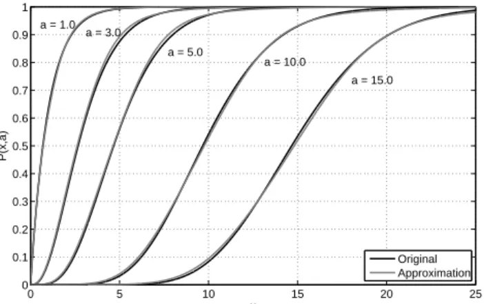
with values monotoneously increasing from 0 forx=0 to 1 forx→ ∞. The majority of the increase from 0 to 1 occurs at values ofxaroundawith a “band width” of about√a(see black curves in Fig. 1, in anticipation of the following).
Taking the complement 1−P (a,x)leads to the so-called upper normalized incomplete gamma function Q(a,x), which, upon multiplication withŴ(a), gives the integral in Eq. (4) but with lower limitx and upper limit∞, which is denoted byγu(a,x). Computing any of γl(a,x), γu(a,x),
P (a,x)orQ(a,x)will lead to any of the other functions by
simple transformations.
Complete and incomplete gamma functions are well-known and treated extensively in the mathematical litera-ture, and there are various ways to compute these functions in practice. To start withŴ(a), along with the well-known recurrence relations, Press et al. (1993) devise a very effi-cient and very accurate approximation fora >0, which is sufficient for cloud microphysical applications, and which has been originally derived by Lanczos (1964). Incomplete gamma functions are analytic for integer values of a (see Eqs. 18–22 later in this paper); for arbitrary values ofa, a widely used method devised again by Press et al. (1993) uses a series expansion ofγl(a,x)or a continued fraction expan-sion ofγu(a,x), depending on whetherxis larger or smaller thana+1. These expansions are summed up to a certain number of terms until convergence is reached. The required number of terms depends onaandx and on the desired nu-merical accuracy.
While this is a very accurate method, the numerical burden is comparatively high within the framework of cloud models and is hard to predict because of the variable number of terms required to reach the desired accuracy, and, on vector ma-chines, this method leads to vectorization problems, which might drastically lower the computing performance. We be-lieve that, among other reasons, these practical problems and the supposedly high computational costs with regard to the low computing performance up to now prevented many cloud physicists from extensively using parametrizations which in-volve incomplete gamma functions, such as Eq. (5). In some cases where incomplete gamma functions have been used, simple analytical approximations for very special and fixed values ofa were employed, e.g., a piecewise linear “ramp” function ofx for non-integera in Cotton et al. (1986). Or, as in Farley et al. (1989), finite integrals similar to the one in Eq. (5) — analytically resulting in incomplete gamma func-tions — have been calculated numerically (which is perhaps even more costly than Press’s method!).
However, if the parameter a is fixed during subsequent function evaluations (as is the case for many cloud micro-physical process parametrizations in the context of bulk
ap-0 5 10 15 20 25
0 0.1 0.2 0.3 0.4 0.5 0.6 0.7 0.8 0.9 1
x
P(x,a)
Original Approximation a = 1.0
a = 3.0
a = 5.0
a = 10.0
a = 15.0
Fig. 1. P (a,x)(black lines) for some values ofaas function of
x. Grey lines: proposed approximation Eq. (12) with coefficients given by Eq. (14) and Table 1.
proaches), the most efficient way in this case is perhaps in-terpolation from pcomputed regular lookup tables with re-spect toxat fixeda. “Regular” is meant here in the sense that the indices of neighbouring table values can be computed from the interpolation point instead of a grid point search. Generally, this is achieved if the distance between tabulated values can be given by some functional form.
Perhaps the most simple example is an equidistant table, where the indices of the neighbouring valuesxi andxi+1in
the table, required to obtain the interpolated value ofγl at a pointx, can be explicitly computed fromx, the starting point
x1of the table and the table increment1x,
i=INT
x −x1 1x
+1. (7)
This is much more efficient and predictable compared to a non-regular table, where a search loop with a nested if-clause is necessary to findi. Another example of a regular lookup table would be logarithmically equidistant.
For the equidistant table, further efficiency is gained by pre-computing the constant 1/1x, so that the costly division is replaced by a cheap multiplication. If linear interpolation between neighbouring table values is used (accuracy might be gained from decreasing1x), so that
γl(x) ≈ γl,i +
γl,i+1−γl,i
1x (x−xi) , (8)
then altogether only one integer rounding operation and a few additions and multiplications have to be performed per
γlevaluation. This method has been used, e.g., by Harringon et al. (1995) and Walko et al. (1995). Alternatively one could use more costly higher order interpolation schemes and at the same time reduce1x.
0 5 10 15 20 25 30 0
5 10 15 20 25 30 35 40 45 50
a x995
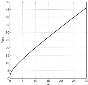
Fig. 2.x995as function ofa.x995is defined byP (a,x995)=0.995.
The necessary span of the table with respect tox at a cer-tain value ofamay be taken from 0 to the valuex995where P (a,x995)=0.995.x995as a function ofamay be estimated
from the approximative formula
x995(a)=g1 1−exp g2a g3 +g4a (9)
g1=36.63 g2= −0.1195
g3=0.3393 g4=1.156
which has been obtained by nonlinear curve fitting and which is depicted in Fig. 2. Atx > x995,P (a,x)≈1 respectively γl(a,x)≈Ŵ(a).
Unfortunately such lookup tables also lead to vectoriza-tion problems because of memory bank conflicts, in case of many parallel vector tasks having to access the same table values at the same time. On such types of architectures, it is desirable to have an approximation formula at hand with a fixed number of mathematical terms, regardless ofa andx. At the same time, for many applications a reduced accuracy may be acceptable, e.g., approximation errors forP within 0.01 absolute and/or 1% relative. Lanczos’s very accurate approximation toŴ(a) does already fulfill the requirement of a fixed number of terms. The purpose of this paper is to develop such an approximation also forγl(a,x), although at a reduced accuracy.
2 Approximation of the lower incomplete gamma function
We seek an approximation by means of nonlinear curve fit-ting, because this leads to the desired fixed number of terms, as opposed to relying on the convergence of series expan-sions. To motivate a regression ansatz, series expansions
are however useful. A series expansion of γl(a,x) can be obtained by plugging the Taylor series of the exponential function exp(−t )into Eq. (4) and integrating each term sep-arately, which leads to (Abramowitz and Stegun, 1970)
γl(a,x) =xa ∞ X
i=0
(−1)i x
i
i!(i+a). (10)
A different well-known representation (e.g., Press et al., 1993) is
γl(a,x) =exp(−x)xa ∞ X
i=0
xi
(a+i)(a+i−1)···a , (11)
which can be obtained from Eq. (10) after tedious manipu-lation by separating the series representation of exp(−x)by means of the Cauchy-product and solving for the series coef-ficients by equating the pre-factors for each individual power ofx.
It turns out that forx≪athe first two terms in Eq. (11) are sufficient to give a reasonable approximation. For largerx, an ever increasing number of terms is necessary. On the other hand, forx→ ∞,P (a,x) approaches 1 seemingly similar to something like 1−c4−x, with some positive number c4.
The former approximation is asymtotically correct forx→
0, the latter forx→ ∞. Therefore, a 4-parametric ansatz
˜
γl(a,x;c1,c2,c3,c4)is constructed which blends the former
function (slightly modified by the the fitting parameterc1)
into the latter:
γl(a,x)≈ ˜γl(a,x)
=exp(−x)xa 1
a+
c1x
a(a+1)+
(c1x)2 a(a+1)(a+2)
!
(1−W (x))+Ŵ(a)W (x) 1−c−4x
(12)
W (x)=1
2+ 1
2tanh(c2(x−c3)) . (13) For many fixed values of a∈ [0.1,30], nonlinear curve fitting by the Levenberg-Marquardt-method with respect to
x∈ [0,x995(a)]leads to a large number of coefficient setsc1
toc4, each coefficient being a function ofa.γ˜l(a,x)denotes the resulting fit, P (a,x)˜ = ˜γl(a,x)/ Ŵ(a) and Q˜ =1− ˜P. The results of such curve fits have been found very pleas-ing, as the absolute approximation errors of the resulting nor-malized functionsP andQare generally less than 0.01 over the employeda-x-domain. This corresponds to a relative er-ror|(P˜−P )/P|<1% forx'aand|(Q˜−Q)/Q|<1% for
x.a. The relative errors might be larger whenP (a,x)and
Q(a,x)approach 0, but relative errors are not meaningful in
Table 1. Coefficientspi,qi,ri, andsi for the approximation functionscˆ1(a). . .cˆ4(a)in Eq. (14).
i pi qi ri si
1 9.4368392235E-03 1.1464706419E-01 0.0 1.0356711153E+00 2 −1.0782666481E-04 2.6963429121E+00 1.1428716184E+00 2.3423452308E+00 3 −5.8969657295E-06 −2.9647038257E+00 −6.6981186438E-03 −3.6174503174E-01 4 2.8939523781E-07 2.1080724954E+00 1.0480765092E-04 −3.1376557650E+00 5 1.0043326298E-01 – – 2.9092306039E+00
6 5.5637848465E-01 – – –
0 5 10 15 20 25 30
0.8 0.85 0.9 0.95 1 1.05 1.1 1.15
Parameter c1 as function of a
a C1
0 5 10 15 20 25 30
0 0.2 0.4 0.6 0.8 1 1.2 1.4 1.6 1.8 2
Parameter c2 as function of a
a C2
0 5 10 15 20 25 30
0 5 10 15 20 25 30 35
Parameter c3 as function of a
a C3
0 5 10 15 20 25 30
0 1 2 3 4 5 6 7 8 9 10
Parameter c4 as function of a
a C4
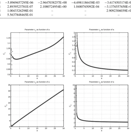
Fig. 3. Numerical values (grey stars) of the regression coefficientsc1throughc4in Eq. (12) as derived by nonlinear regression for fixed
values ofa. Black lines: nonlinear regression functions to each ofc1throughc4as functions ofaafter ansatz (14) and the coefficients from
Table 1.
As a last step,c1toc4are approximated as functions ofa,
again by nonlinear curve fitting. The results are
c1(a)≈ ˆc1(a) = 1 +p1a +p2a2 +p3a3 +p4a4
+p5(exp(−p6a)−1) (14)
c2(a)≈ ˆc2(a) = q1+ q2
a +
q3 a2+
q4
a3 (15)
c3(a)≈ ˆc3(a) = r1 +r2a + r3a2 +r4a3 (16)
c4(a)≈ ˆc4(a) = s1 + s2
a +
s3 a2+
s4 a3+
s5
a4, (17)
where the particular functional forms have been arrived at by guessing and experimentation. The values for the parameters
p1. . .p6,q1. . .q4,r1. . .r4ands1. . .s5are given in Table 1.
Replacing in Eq. (12)c1. . .c4bycˆ1. . .cˆ4leads to the final
approximationγˆl(a,x). Figure 1 shows examples of the nor-malizedP (a,x)ˆ = ˆγl(a,x)/ Ŵ(a)(grey lines) as function ofx for some fixed values ofain comparison to the original
func-tionP (a,x)(black lines), demonstrating a reasonably good
agreement.
However, Fig. 3 shows the coefficientsc1toc4as obtained
by the curve fits at constant a (grey stars) along with the corresponding approximationscˆ1 . . .cˆ4given by Eqs. (14)–
(17) (black lines), and some difficulties at the lower range ofa-values (a <0.9) are apparent. Therefore,γˆl(a,x)(resp.
ˆ
−0.03 −0.02
−0.02
−0.01
−0.01
0
0
0
0
0
0.01
0.01
0.01
0.01
0.02
0.02
0.02
0.02
0.03
0.03
0.04
0.04
0.05
0.05
0.1
0.1
0.51 10
a
x / (a + 1)
Relative error for P(a,x)
0 5 10 15 20 25 30
0 0.5 1 1.5 2 2.5
−0.02
−0.015
−0.015
−0.01
−0.01
−0.005
−0.005
−0.005
−0.005
−0.005
0
0
0
0
0
0.005
0.005
0.005
0.005 0.005
0.005 0.01
0.01
0.01
0.01
0.01
0.015
0.015
0.015
0.02
0.025
0.030.035
0.040.0450.05
a
x / (a + 1)
Absolute error for P(a,x)
0 5 10 15 20 25 30
0 0.5 1 1.5 2 2.5
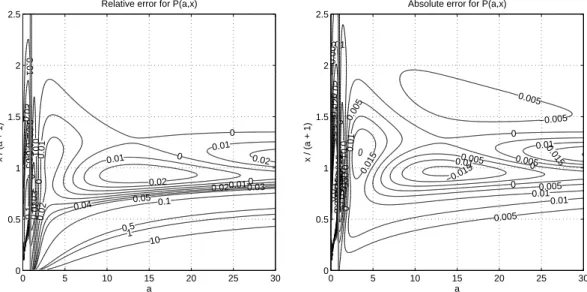
Fig. 4. Relative (left) and absolute (right) error of the proposed approximationP (a,x)ˆ = ˆγ(a,x)/ Ŵ(a)as function ofaandx/(a+1). The parameterxhas been scaled bya+1 because the main variation ofP (a,x)withxtakes place atx-values arounda+1. The vertical grey lines ata=0.9 indicate the lower boundary with respect toaof the(a,x)-range where errors are acceptable.
a <0.9, a fact that is clearly demonstrated in Fig. 4, which depicts the relative and absolute errors(Pˆ−P )/P(left plate) andPˆ−P (right plate) as function ofaandx. In these fig-ures,xhas been scaled bya+1 sinceP varies mostly in the region ofxarounda+1.
Where do these difficulties for small values of a come from? To understand this, it is instructive to look at the ana-lytical formulas forγl(a,x)in case ofa being an integerm, starting withm=1,
γl(1,x)=1 −e−x (18)
γl(2,x)=1 −(x+1)e−x (19)
γl(3,x)=2 −(x2+2x+2)e−x (20)
γl(4,x)=6 −(x3+3x2+6x+6)e−x (21)
.. .
γl(m,x)=
h
−tm−1e−tix
0 +(m−1)
x Z
0
tm−2e−tdt
= −xm−1e−x +(m−1)γl(m−1,x)
=Ŵ(m)−
m−1
X
i=0 di dxi
xm−1
!
e−x. (22)
The last finite sum representation has been deduced from the representations atm=1,2,...and can be proved by a) taking the first derivative with respect tox, which yieldsxm−1e−x
as it should, and b) by the fact that the highest derivative (last element in the sum) equals(m−1)!(which isŴ(m)), so that forx=0 the correct valueγl(m,0)=0 is obtained. For small integer values ofm, this representation is an efficient way to evaluateγl.
Now, concerning the difficulties for small values ofa,γl for a= 1 (Eq. 18) is a simple exponential function which matches the ansatz (12) only in the limitsc2→ ∞,c3=0
andc4=e. Asa→1, the coefficientsc2toc4 go towards
these values, as is shown in Fig. 3, with the singularity of
c2at a=1. Of course ata=1 the fitting algorithm leads
to a “compromise”-solution with finitec2; otherwise, a kind
of branch-cut of the coefficients around a=1 can be ob-served. For larger values ofa, the analytical formulation of
γlgets more complicated (forabeing an integerm, more and more terms get involved into the finite sum in Eq. (22) asm
increases) and is more likely to be well describable by the
ansatz (12).
For most cloud microphysical applications, the branch for
a >1 seems to be the important one. Therefore, the approx-imations (14)–(17) are developed to represent mainly that branch. By altering the regression functions to, e.g., rational functions, it would perhaps be possible to find approxima-tions which encompass both branches.
It turns out, however, that the approximations (14)–(17) are applicable for a-values down to 0.9, because for a≥
0.9, the absolute error | ˆP−P| given in Fig. 4 (right fig-ure) remains below 0.02 everywhere, and the relative error
|(Pˆ−P )/P|(left figure) is also quite small except whenP
gets close to 0. But here, the relative error is not a good error measure anyways. Beyond the range ofa-values for which
ˆ
P has been fitted, it turns out that the approximation error remains within the same small limits up toa=45. Above that,Pˆis not a good approximation.
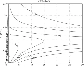
A further condition forPˆ to be of practical use is that this function increases monotonically with respect to increasingx
0.001
0.001
0.001
0.01
0.01
0.01
0.05
0.05
0.05
0.1
0.1
0.2
0.5
1
1
a
x / (a + 1)
∂ P(a,x) / ∂ x
0 5 10 15 20 25 30
0 0.5 1 1.5 2 2.5
Fig. 5. ∂P (a,x)/∂xˆ =1/ Ŵ(a)∂γˆl(a,x)/∂x as function ofa and
x/(a+1). Same scaling ofxand same grey line as in Fig. 4.
check monotonicity is to look at the sign of the partial deriva-tive ofPˆ with respect tox. Figure 5 shows∂P (a,x)/∂xˆ =
1/ Ŵ(a) ∂γˆl(a,x)/∂x (the formula is omitted for brevity) as function ofa andx, and it is apparent that values are>0 everywhere, which indicates the desired monotonicity.
Concerning the efficiency of the proposed approximation, it has been found that, on our scalar linux desktop computer using the gfortran compiler and high optimization, it is faster by a moderate factor 4 on average compared to the efficient method of Press et al. (1993) mentioned in the introduction. Here, the speed-up depends onaandx, that is, on the number of required terms and the desired accuracy in Press’s method. The latter has not been changed from its original values.
A more impressive speed-up is gained, however, in the case where subsequent evaluations at the same value of a
are needed, as is the case in cloud physics: many coefficients of the terms in the proposed approximation only depend ona
and may be pre-computed once, so that we were able to ob-tain a speed-up factor of about 15 on average. But the biggest advantage is perhaps on vector CPUs, where the fixed num-ber of terms makes vectorization easy for programmers and compilers. Also, there might be advantages on massively parallel machines in that the method avoids load imbalances otherwise caused by different numbers of terms in series ex-pansions to reach convergence at different grid points.
Further experiments, in which the hyperbolic tangent in Eq. (12) has been replaced by the simple but accurate and continuously differentiable rational approximation
tanh(x)≈
−1 x≤ −c3t
9c2tx+27x3 c3t+27ctx2 −
ct 3<x<
ct
3 ct=9.37532
1 x≥c3t
(23)
did not increase efficiency on our desktop computer. This is presumably because the necessary numerical division ope-ration is very costly and because the tanh-function is al-ready implemented in a very efficient way in state-of-the-art compilers. Nevertheless, if on a specific computer system the computation of tanh should cause efficiency problems, Eq. (23) might be tried instead. Observe that changing the value forct would only rescale the function along the x-axis but preserve the differentiability and the “outer” function va-lues−1 and 1, a fact that renders Eq. (23) a quite general blending function.
3 Summary
This paper describes an approximation to the lower incom-plete gamma function which has been obtained by nonlin-ear curve fitting. It comprises a fixed number of terms and yields moderate accuracy (absolute approximation error of
P is <0.02 in the range 0.9≤a≤45 and x≥0), which should be enough for most cloud microphysical applications, but may be problematic for other applications. The proposed approximation Pˆ consists of Eq. (12) in combination with Eqs. (14)–(17) and coefficients given in Table 1. Mono-tonicity and asymptotic behaviour of the original incomplete gamma functions are preserved, which is important.
The method is generally only slightly more efficient in terms of the required number of floating point operations than the more accurate method of Press et al. (1993), but if subsequent evaluations at a certain fixed value of a are sought (which is often the case in cloud microphysics), then a significant performance increase can be obtained by pre-computing certain terms and coefficients which only depend on a. On scalar architectures, however, the most efficient method to evaluate incomplete gamma functions is certainly interpolation of regular lookup tables as described in the in-troduction.
A great advantage of the proposed approximationPˆ is its applicability on vector CPUs, because the formula with its fixed number of terms is well suited for vectorization, as op-posed to, e.g., Press’s method or other more accurate algo-rithms based on series- or continued-fraction representations. With regard to massively parallel machines (where the use of equidistant lookup tables might pose memory issues), the fixed number of terms might be also beneficial to avoid load imbalances caused by different numbers of terms in series expansions to reach convergence at different grid points.
Acknowledgements. This work has been inspired by discussions
with Axel Seifert (German Weather Service), who also suggested some improvements to the manuscript. Very valuable comments of two anonymous referees helped to improve and clarify the manuscript.
References
Abramowitz, M. and Stegun, I. A.: Handbook of Mathematical Functions with Formulas, Graphs, and Mathematical Tables, Dover Publications, 1970.
Chandrasekar, V. and Bringi, V. N.: Simulation of Radar Reflec-tivity and Surface Measurements of Rainfall, J. Atmos. Ocean. Tech., 4, 464–478, 1987.
Cotton, W. R., Tripoli, G. J., Rauber, R. M., and Mulvihill, E. A.: Numerical Simulation of the Effects of Varying Ice Crystal Nu-cleation Rates and Aggregation Processes on Orographic Snow-fall, J. Appl. Meteorol., 25, 1658–1680, 1986.
Deirmendjian, D.: Far-Infrared and Submillimeter Wave Attenu-ation by Clouds and Rain, J. Appl. Meteorol., 14, 1584–1593, 1975.
Farley, R. D., Price, P. E., Orville, H. D., and Hirsch, J. H.: On the Numerical Simulation of Graupel/Hail Initiation via the Riming of Snow in Bulk Water Microphysical Cloud Models, J. Appl. Meteorol., 28, 1128–1131, 1989.
Harringon, J. Y., Meyers, M. P., Walko, R. L., and Cotton, W. R.: Parameterization of ice Crystal Conversion Processes Due to Va-por Deposition for Mesoscale Models Using Double-Moment Basis Functions. Part 1: Basic Formulation and Parcel Model Results, J. Atmos. Sci., 52, 4344–4366, 1995.
Illingworth, A. J. and Blackman, T. M.: The Need to Represent Raindrop Size Spectra as Normalized Gamma Distributions for the Interpretation of Polarization Radar Observations, J. Appl. Meteorol., 41, 286–297, 2002.
Lanczos, C.: A Precision Approximation of the Gamma Function, J. SIAM Numer. Anal. Ser. B, 1, 86–96, 1964.
Lin, Y.-L., Farley, R., and Orville, H.: Bulk Parameterization of the Snow Field in a Cloud Model, J. Clim. Appl. Meteorol., 22, 1065–1092, 1983.
Locatelli, J. D. and Hobbs, P. V.: Fall Speeds and Masses of Solid Precipitation particles, J. Geophys. Res., 79, 2185–2197, 1974.
Milbrandt, J. A. and Yau, M. K.: A Multimoment Bulk Micro-physics Parameterization. Part I: Analysis of the Role of the Spectral Shape Parameter, J. Atmos. Sci., 62, 3051–3064, 2005a. Milbrandt, J. A. and Yau, M. K.: A Multimoment Bulk Micro-physics Parameterization. Part II: A Proposed Three-Moment Closure and Scheme Description, J. Atmos. Sci., 62, 3065–3081, 2005b.
Press, W. H., Teukolsky, S. A., Vetterling, W. T., and Flannery, B. P.: Numerical Recipes in Fortran 77, Cambridge University Press, 1993.
Pruppacher, H. R. and Klett, J. D.: Microphysics of Clouds and Precipitation, 2nd edn., Kluwer Academic Publishers, Dordrecht, Boston, London, 1997.
Seifert, A. and Beheng, K. D.: A Two-Moment Cloud Microphysics Parameterization for Mixed-Phase Clouds. Part I: Model De-scription, Meteorol. Atmos. Phys., 92, 45–66, 2006.
Seifert, A.: On the Parameterization of Evaporation of Raindrops as Simulated by a One-Dimensional Rainshaft Model, J. Atmos. Sci., 65, 3608–3619, 2008.
Testud, J., Oury, S., Black, R. A., Amayenc, P., and Dou, X.: The Concept of “Normalized” Distribution to Describe Raindrop Spectra: A Tool for Cloud Physics and Cloud Remote Sensing, J. Appl. Meteorol., 40, 1118–1140, 2001.
Walko, R. L., Cotton, W. R., Meyers, M. P., and Harrington, J. Y.: New RAMS Cloud Microphysical Parameterization. Part I: The Single-Moment Scheme, Atmos. Res., 38, 29–62, 1995. Willis, P. T.: Functional Fits to Some Observed Drop Size
Distri-butions and Parameterization of Rain, J. Atmos. Sci., 41, 1648– 1661, 1984.
Young, K. C.: Microphysical Processes in Clouds, Oxford Univer-sity Press, 1993.