www.geosci-model-dev.net/6/1925/2013/ doi:10.5194/gmd-6-1925-2013
© Author(s) 2013. CC Attribution 3.0 License.
Geoscientiic
Model Development
A bulk parametrization of melting snowflakes with explicit liquid
water fraction for the COSMO model
C. Frick1,2, A. Seifert2,3, and H. Wernli1
1Institute for Atmospheric and Climate Science, ETH Zurich, Switzerland 2Deutscher Wetterdienst, Offenbach, Germany
3Hans Ertel Centre for Weather Research, Hamburg, Germany
Correspondence to:C. Frick ([email protected])
Received: 4 April 2013 – Published in Geosci. Model Dev. Discuss.: 21 May 2013 Revised: 28 August 2013 – Accepted: 4 October 2013 – Published: 6 November 2013
Abstract.A new snow melting parametrization is presented for the non-hydrostatic limited-area COSMO (“consortium for small-scale modelling”) model. In contrast to the stan-dard cloud microphysics of the COSMO model, which in-stantaneously transfers the meltwater from the snow to the rain category, the new scheme explicitly considers the liquid water fraction of the melting snowflakes. These semi-melted hydrometeors have characteristics (e.g., shape and fall speed) that differ from those of dry snow and rain droplets. Where possible, theoretical considerations and results from vertical wind tunnel laboratory experiments of melting snowflakes are used as the basis for characterising the melting snow as a function of its liquid water fraction. These characteristics include the capacitance, the ventilation coefficient, and the terminal fall speed. For the bulk parametrization, a critical di-ameter is introduced. It is assumed that particles smaller than this diameter, which increases during the melting process, have completely melted, i.e., they are converted to the rain category. The values of the bulk integrals are calculated with a finite difference method and approximately represented by polynomial functions, which allows an efficient implementa-tion of the parametrizaimplementa-tion. Two case studies of (wet) snow-fall in Germany are presented to illustrate the potential of the new snow melting parametrization. It is shown that the new scheme (i) produces wet snow instead of rain in some regions with surface temperatures slightly above the freezing point, (ii) simulates realistic atmospheric melting layers with a gradual transition from dry snow to melting snow to rain, and (iii) leads to a slower snow melting process. In the fu-ture, it will be important to thoroughly validate the scheme, also with radar data and to further explore its potential for improved surface precipitation forecasts for various meteo-rological conditions.
1 Introduction
Accurate prediction of surface snowfall is a particularly chal-lenging aspect of numerical weather prediction (NWP). It re-quires capturing the general dynamics leading to cloud and precipitation formation, and a meaningful representation of microphysical processes by cloud parametrizations. Partic-ularly difficult are surface precipitation predictions in situ-ations with near-surface temperatures slightly above 0◦C, when snowflakes start to melt before reaching the ground (e.g., Frick and Wernli, 2012). In such situations, slight er-rors in the vertical temperature and humidity structure and/or in the parametrization of the melting process can lead to a misforecast of the surface precipitation type (rain instead of snow or vice versa). Thériault et al. (2006) highlighted the great importance of the vertical temperature structure and Matsuo and Sasyo (1981) the impact of humidity for the re-sulting precipitation type. High values of relative humidity lead to an accelerated melting process while for low values the cooling due to sublimation of snow delays the onset of melting. The melting itself also influences the thermodynam-ics of the atmosphere due to the associated latent cooling (e.g., Raga et al., 1991). Lin and Stewart (1986) described perturbations due to cooling by melting snow that might lead to mesoscale thermal circulations. Additionally, Szyrmer and Zawadzki (1999) identified horizontal variabilities of atmo-spheric properties in the melting layer that are able to initiate convective cells.
The present study focuses on the numerical implementation of the melting process of snowflakes. In general, frozen hy-drometeors start melting when their surface temperature ex-ceeds 0◦C (Mitra et al., 1990). The melting process is not instantaneous and extends over a layer of several hundred metres for completely converting a snowflake into a raindrop (Mitra et al., 1990). The region in which this transition oc-curs is called the melting layer and has been intensively in-vestigated (e.g., Bocchieri, 1980; Czys et al., 1996; Rauber et al., 2001). This layer consists of partially melted particles, which have specific characteristics that differ from the ones of dry snow and rain, e.g., in terms of shape and fall velocity. In radar observations the partially melted hydrometers of the melting layer lead to a band of enhanced radar reflectivity, the so-called “bright band”. This phenomenon has been well described and investigated (e.g., Austin and Bemis, 1950; Yokoyama and Tanaka, 1984; Fabry and Zawadzki, 1995; Braun and Houze, 1995; Fabry and Szyrmer, 1999).
The melting of single snowflakes has been investigated in several laboratory studies (e.g., Matsuo and Sasyo, 1981; Mi-tra et al., 1990) and field experiments (e.g., Knight, 1979; Fujiyoshi, 1986; Barthazy et al., 1998). The findings of these studies provide the background for the numerical description of the melting process and its implementation into bulk mi-crophysical parametrizations of NWP models. For the usage in operational NWP models the process is typically highly simplified, for instance by converting the meltwater gener-ated within one time step instantaneously into rain. As a con-sequence, most schemes cannot represent partially melted snowflakes, which might affect the interaction between the melting process and the vertical profiles of temperature and humidity, and lead to erroneous fall speeds and an accel-erated melting process. In a recent case study of a poorly predicted, high-impact wet snowfall event in northwestern Germany in November 2005, Frick and Wernli (2012) illus-trated the difficulty in simulating such events with conven-tional snow melting schemes. Also when predicting the ver-tical temperature profile fairly realisver-tically, the melting pro-cess in the considered NWP models was too fast leading to a prediction of surface rain instead of wet snow. Additionally, such a simplified treatment of the melting process in NWP models impedes a direct comparison between model data and radar observations in situations with a bright band.
The objective of this study is to develop a new melt-ing parametrization that is able to represent wet snowflakes for the COSMO model (for more information about the COSMO model see, e.g., Doms and Schättler, 2002, or visit www.cosmo-model.org). If successfully implemented into the COSMO model, such a scheme might lead to improved snowfall predictions under melting conditions and the model data can be more easily compared and validated with radar observations of the “bright band”. In Sect. 2, the develop-ment of the new parametrization is described, starting with the melting behaviour of a single snowflake (Sect. 2.2). The bulk approach for considering an ensemble of snowflakes is
presented in Sect. 2.3 and its implementation in the COSMO model version 4.14 in Sect. 2.4. The source code of the presented parametrization is available from the authors. In Sect. 3, some first results are presented to illustrate the differ-ences in surface precipitation between simulations using the new and the standard melting scheme. Note that these results mainly provide an impression of the new scheme’s potential; however a thorough validation of the new scheme is beyond the scope of this study and the subject of future investigation.
2 Model description
2.1 Modelling concept
The melting of snowflakes can be described based on the en-ergy budget of an individual melting snowflake. It follows that the mass change of the corresponding meltwater above the temperatureT0=273.15 K is given by (e.g., Mitra et al., 1990; Pruppacher and Klett, 1997)
dmw dt
melt=
4π CsFv LF
lh1T+ LvDv
Rv 1q
(1) with1T =T−T0whereT is the temperature of the air, and 1q=e/T−es,w(T0)/T0whereegives the vapour pressure andes,wthe saturation vapour pressure over water.LF is the
latent heat of melting,Lvthe latent heat of evaporation,lhthe diffusivity of heat,Dvthe diffusivity of water vapour, andRv the gas constant of water vapour. The left term in the brackets represents the contribution to melting due to diffusional heat transport and the right term accounts for evaporation. The ventilation coefficientFvand the capacitanceCs depend on the snowflake characteristics while the remaining part of the equation is a function of the ambient air conditions.
Most bulk microphysical parametrizations make the sim-plyfing assumption thatCsandFvonly depend on the char-acteristic diameter (e.g., maximum dimension) Ds of the snowflake. In this case, Eq. (1) can be written as
dmw dt
melt=
G(T , e) Cs(Ds) Fv(Ds), (2) where G(T , e) is a function that combines the thermody-namic, i.e., environmental parameters. For a bulk microphys-ical parametrization this rate equation has to be integrated for an ensemble of snowflakes. Usually it is assumed that the number density distribution of snowflakes can be described by an exponential or Gamma distribution, e.g.,
f (D)=N0Dµexp(−λD), (3)
2005) found exponential distributions in geometric diameter Ds. The preference for one or the other might simply be due to different measurement devices. Most bulk parametrization use Eq. (3) with geometric diameterDswhich simplifies the formulation of the collection rates. We follow the latter ap-proach and useDsin Eq. (3). Second, the exponentµhas to be considered. For the calculation of mass changes, an ex-ponential distribution, i.e.,µ=0, is a reasonable assump-tion for the number density distribuassump-tion because the mass-weighted part of the spectrum is more dominant. Therefore, we apply an exponential distribution (µ=0) in geometric di-ameterDsfor the number density distribution of snowflakes. Large snowflakes are mostly aggregates of crystals and therefore it is well founded to expect a ms∼Ds2 relation (Westbrook et al., 2004a, b). More specifically we assume ms=αDs2 with α=0.069 kg m−2 (Wilson and Ballard, 1999; Field et al., 2005). The snow water content of snowflakesLs, and the mixing ratioqsare then given by
Ls=ρqs=
∞
Z
0
msf (Ds)dDs, (4)
withρfor the density of air. The resulting mass change due to melting for an ensemble of snowflakes is calculated from
∂Ls ∂t
melt = −
∞
Z
0 dmw
dt
melt
f (Ds)dDs
= −G(T , e) ∞
Z
0
Cs(Ds) Fv(Ds) f (Ds)dDs. (5)
The integral can be solved analytically and yields the mass change of the ensemble of snowflakes. In almost all bulk microphysical parametrizations the meltwater produced by Eq. (5) is instantaneously converted into rain (Lin et al., 1983; Rutledge and Hobbs, 1984; Cotton et al., 1986; Fer-rier, 1994; Mölders et al., 1995; Reisner et al., 1998; Morri-son et al., 2005; Seifert and Beheng, 2006; Lim and Hong, 2010). In these schemes, there is no internal mixing of liquid and solid water within the snow category, i.e., no separate prognostic variable for the meltwater on snowflakes. Meyers et al. (1997) discussed various attempts to fix the inherent problems of bulk melting schemes. This simplification leads to errors in the prediction of snowfall, the thermodynamics of the melting layer, and might lead to misforecasts of sur-face snowfall (Frick and Wernli, 2012), as already described in Sect. 1.
The conceptional idea of the new melting scheme is to al-low the representation of partially melted snowflakes, which leads to a splitting of the mass of an individual snowflakems into a liquid partmw and a solid part mi, i.e., the melting snowflake has a liquid water fraction
ℓ=mw ms =
mw mi+mw
. (6)
The melting snowflakes are represented by an internal mixture of liquid water and ice instead of having just exter-nally mixed rain and snow categories.
Of course, the formulation of a model using internally mixed melting snowflakes and the incorporation in a bulk scheme is not straightforward. To our knowledge the only bulk parametrization including such an approach is the scheme of Szyrmer and Zawadzki (1999, SZ99 hereafter). For spectral bin models, where the implementation of a prog-nostic meltwater is considerably easier, Phillips et al. (2007) describe such a prognostic melting scheme. Our new scheme follows SZ99 with the main modification that we use the bulk meltwater mixing ratio instead of the critical diameter as the additional prognostic variable, which helps to ensure mass conservation and makes the implementation in a three-dimensional model more consistent.
The following subsections describe the parametrizations of the properties of individual melting snowflakes, the for-mulation of the bulk scheme, and the implementation in the COSMO model.
2.2 Individual melting snowflakes
Following Mitra et al. (1990, M90 hereafter), who performed extensive laboratory studies on the melting of snowflakes in a vertical wind tunnel, the melting process of a single snowflake with included meltwater can be completely de-scribed.
The mass change of the meltwater of an individual snowflake above the critical surface temperature can be writ-ten as
dmw dt
melt
=G(T , e) Cm(Ds, ℓ) Fv(Ds, ℓ) (7)
following Eq. (2) of M90. As for a snowflake without melt-water, cf. our Eq. (2),G(T , e)only depends on the ambient air conditions, while capacitanceCmand ventilation coeffi-cientFvof the melting snowflake depend on the maximum dimensionDsof the mass equivalent dry snowflake and the liquid water fractionℓ. Based on their laboratory results M90 provide parametrizations of these parameters with the addi-tional dependency onℓ.
For the calculation of the capacitance M90 applied the ap-proximation for an oblate spheroid. The axis ratio is assumed to be 0.3 for a dry dendritic crystal, and 1.0 for a raindrop. The axis ratio for melting snowflakes is approximated by a linear interpolation, i.e.,
a(ℓ)=0.3+0.7ℓ (8)
and the capacitance is then given by Pruppacher and Klett (1997, p. 547, Eq. 13–78),
Cm(Ds, ℓ)=αcap(ℓ)
Dm(Ds, ℓ) 2
p
1−a(ℓ)2
a) capacitance b) fall velocity
c) ventilation coefficient d) empirical function
Fig. 1. (a)Capacitance,(b)fall velocity, and(c)ventilation coefficient of a melting snowflake as a function of the equivalent diameter for various values ofℓ. Rain and snow correspond toℓ=1 andℓ=0, respectively.(d)Empirical function9(ℓ)that describes the transition between the fall speed of a snowflake and a raindrop. Shown are the approximate relationship Eq. (15) and the original data (grey dots) of Mitra et al. (1990).
withCm(Ds,0)=CsandCm(Ds,1)=Cr.Dmis the maxi-mum dimension of the melting snowflake, which can be cal-culated as follows
Dm(Ds, ℓ)=
6ms π a(ℓ)ρm(Ds, ℓ)
1/3
(10) assuming an oblate spheroid shape of the melting snowflake (see above) and in agreement with Eq. (8) of M90. Hereρmis the density of the melting snowflake. As suggested by M90, we interpolateρm(Ds, ℓ) between the density of liquid wa-ter,ρw=1000 kg m−3, and the density of the dry snowflake ρs(Ds, ℓ):
ρm(Ds, ℓ)=ρs(Ds, ℓ)+(ρw−ρs(Ds, ℓ))ℓ. (11)
For the density of a dry snowflake with the axis ratio of the melting snowflake it follows from the assumption of the oblate spheroid shape that
ρs(Ds, ℓ)= 6ms π D3
sa(ℓ)
, (12)
but only until a maximum value ofρs=500 kg m−3because higher densities are not reasonable for snowflakes. The em-pirical correction factorαcap(ℓ)in Eq. (9) is about 0.8 for dry snowflakes and for melting snowflakes M90 again suggest a linear interpolation, i.e.,
The resultingCm is shown in Fig. 1a for various values ofℓ. With increasing diameter, the capacitance of dry snow increases faster than the one of rain and the capacitance of partially melted particles follows the interpolation between both. M90 have shown that such a simple model for the ca-pacitance is sufficient to achieve a good agreement with the experimental data.
Another important result of M90 is that the terminal fall velocity of a melting snowflake can be parameterized by vm(Ds, ℓ)=vs(Ds)+ [vr(Dr)−vs(Ds)]9(ℓ), (14) wherevs andvr are the terminal fall velocities of the mass
equivalent dry snowflake and raindrop, which we calcu-late following Khvorostyanov and Curry (2005, KC05 here-after). Both depend on the corresponding maximum dimen-sions which are in fact functions of the mass equivalent di-ameter Deq of a liquid sphere. For the calculation of the maximum dimension of the raindrop fromDeq we follow Khvorostyanov and Curry (2002). For dry snowflakesDs is calculated by usingms=(π/6) ρwDeq3 andDs=(ms/α)1/2 with α=0.069 and, in addition, a cross sectional area of A=0.45π/4Ds2 is assumed following Field et al. (2008). The empirical function9(ℓ)is given by Fig. 2 of M90. An approximation for9(ℓ)derived from the measurements is
9(ℓ)=α9ℓ+(1−α9) ℓ7 (15)
withα9=0.246, as shown in Fig. 1d. The resulting fall ve-locity of a melting snowflake is presented in Fig. 1b. As in-dicated by the empirical function9(ℓ), the fall velocity of a melting snowflake shows a slow linear increase for small ℓ, but increases rapidly to the one of a raindrop forℓlarger than 0.7. The resulting sedimentation velocity of a melting snowflake is necessary to describe the sedimentation process, but also affects the melting process due to the ventilation co-efficient.
For the determination of the ventilation coefficient of a melting snowflake our definition of the length scale in the Reynolds number deviates from M90. Instead we are consis-tent with KC05 and others in using the maximum dimension of the particle. For large snowflakes or raindrops the drag co-efficient becomes approximately constant. In this large par-ticle limit the Reynolds number is only a function of mass, i.e.,
NRe(D)=
D v(D)
νa ∼
√
m (16)
with νa the kinematic viscosity of air, and therefore the
Reynolds number of a melting snowflake NRe(Ds, ℓ) does not change strongly during the melting process. This mo-tivates us to calculate the Reynolds number of melting snowflakes by linear interpolation w.r.t.ℓbetween the mass equivalent dry snowflake and raindrop, instead of trying to come up with a more complicated model for the particle den-sity or the geometry of a melting snowflake, which would be
necessary to calculateNRe(Ds, ℓ)explicitly. Having an ap-proximation for the Reynolds number of the particle the ven-tilation coefficient is calculated using the empirical formula of Hall and Pruppacher (1976)
Fv(Ds, ℓ)=
(
1.00+0.14X2(Ds, ℓ), for X <1 0.86+0.28X(Ds, ℓ), else
(17)
withX(Ds, ℓ)=N 1/3
Sc N
1/2
Re (Ds, ℓ)and the Schmidt number NSc=0.64 consistent with M90. The resulting ventilation
coefficient is shown in Fig. 1c as a function of the equivalent diameter. The ventilation coefficients for rain and snow are nearly equal, meaning that a dry snowflake has nearly the same ventilation coefficient as the mass equivalent raindrop. With this parametrization all terms of Eq. (7) are specified and therefore the melting process of an individual snowflake is completely described.
2.3 Bulk parametrization
In a scheme with a prognostic liquid water fraction, the mass msof an individual snowflake is decomposed into an ice part miand a liquid partmw. Therefore, we define
Ls,i=ρqs,i =
∞
Z
D∗
mi(Ds) fm(Ds, ℓ)dDs (18)
Ls,w=ρqs,w=
∞
Z
D∗
mw(Ds) fm(Ds, ℓ)dDs (19)
for the bulk content of ice and meltwater of the wet snowflakes. Note that mi and mw are in general functions ofDs since snowflakes of different sizes have different liq-uid water fractions. Here we assume that snowflakes smaller thanD∗ have already melted completely and are no longer snowflakes, but raindrops, as discussed later. In addition, the size distribution of melting snowflakesfm(Ds, ℓ)becomes a function of the liquid water fraction.
Using Eq. (7) we find the rate equation
∂Ls,w ∂t
melt =
∞
Z
D∗ dmw
dt
melt
fm(Ds, ℓ)dDs
=G(T , e) ∞
Z
D∗
Cm(Ds, ℓ) Fv(Ds, ℓ) fm(Ds, ℓ)dDs. (20)
From the previous section, we already know Cm(Ds, ℓ) andFv(Ds, ℓ), i.e., Eqs. (9) and (17). To evaluate the inte-gral on the r.h.s. we have to further specify
1. the liquid water fraction of individual snowflakes ℓ(Ds);
3. the threshold diameterD∗of the distribution.
Using a bulk approach we predict only the bulk quantities Ls,iandLs,w, not the size-resolvedℓitself. Following SZ99, we assume
ℓ(Ds)∼=
D∗
Ds
̹
. (21)
They showed that approximatelyℓ∼D− ˜eq̹ with̹˜=1.3, cf. their Eq. (18), and with Deq3 ∼Ds2 it follows ̹= 2/3̹˜=0.87. This approach takes into account that smaller snowflakes melt faster than larger particles (e.g., Willis and Heymsfield, 1989).
To specify the size distribution of melting snowflakes we follow, again, SZ99 and use that in steady state the number flux at a certain melted diameter is constant with height due to mass conservation. BecauseDs is the maximum dimen-sion of the dry mass equivalent snowflake, not the maximum dimension of the melting snowflake,Dsis in fact a mass co-ordinate and number flux conservation can be written as fm(Ds, ℓ)=
vs(Ds) vm(Ds, ℓ)
f (Ds). (22)
In contrast to SZ99 we do not attempt to match both the snow distribution above and the raindrop distribution be-low the melting layer, because for size distributions of dry snow, which are exponential in geometric diameter rather than melted diameter, such a matching is not exactly pos-sible using the flux conservation alone. Therefore, we decide to match the distribution of melting snow to the distribution of dry snow only. For the size distribution of dry snow we use, for simplicity, the local value of the snow water content, i.e.,λis a function ofLs=Ls,i+Ls,w. Note that by doing so we chose to build a local scheme. Alternatively, one could try to estimate the snow content of the unmelted distribution above. In a time-dependent 3-D framework both approaches are, of course, approximations.
The critical diameterD∗can be calculated iteratively from the local values ofLs,iandLs,wfor a given set of parameters N0andλ, i.e., fromLs=Ls,i+Ls,wandN0one can calculate λ, and thenD∗iteratively from Eq. (18). This cumbersome inversion problem is maybe one reason why prognostic melt-ing schemes have not become very popular so far.
Figure 2 illustrates the described size distributions for a snow mixing ratio of 3 g kg−1and a value of 0.2 for the bulk liquid water fraction. The decrease of meltwater from smaller to larger snowflakes and the behaviour of the corresponding ice part illustrate well the effect of the size resolved liquid water fraction ℓ(Ds). Vertical lines mark the evolution of D∗ within one time step and therefore the conversion from snow to rain. The critical diameter of the melting snow size distributionD∗ represents the size of the smallest predicted snowflakes. Smaller snowflakes have already melted pletely due to the fact that small snowflakes melt faster com-pared to larger ones. Therefore,D∗increases during melting
Ds (cm)
siz
e distr
ib
ution (m
−
3 cm
−
1 )
0.0 0.1 0.2 0.3 0.4 0.5 102
103 104
dry snow melting snow melt water ice water D*
Fig. 2. Size distributions obtained with the new melting parametrization using a bulk liquid water fraction of 0.2 and a snow mixing ratio of 3 g kg−1. The two values ofD∗ (indicated by the vertical dashed lines) illustrate a shift of the critical diameter due to the conversion from snow to rain.
and this shift yields the conversion rate from snow to rain:
∂Ls,w ∂t
conv=
lim
1t→0
1
1t
D∗(t+1t )
Z
D∗(t )
mw(Ds) fm(Ds, ℓ)dDs. (23)
How we evaluate this integral will be discussed at the end of the next section.
Having specified the fall speeds of melting snowflakes vm(Ds, ℓ)in the previous section the calculation of the bulk sedimentation velocities is straightforward:
¯ vs,i =
1 Ls,i
∞
Z
D∗
mi(Ds, ℓ) vm(Ds, ℓ) fm(Ds, ℓ)dDs
= α
Ls,i
∞
Z
D∗
(1−ℓ) vm(Ds, ℓ) fm(Ds, ℓ) D2sdDs (24)
¯ vs,w=
1 Ls,w
∞
Z
D∗
mw(Ds, ℓ) vm(Ds, ℓ) fm(Ds, ℓ)dDs
=Lα s,w
∞
Z
D∗
ℓ vm(Ds, ℓ) fm(Ds, ℓ) Ds2dDs (25)
2.4 Implementation in the COSMO model
In the two-category mixed-phase cloud microphysical scheme which is currently used operationally in the COSMO model the parametrization of the melting process of snow (see also Sect. 2.1) is based on an approximate form of the rate equation (Doms and Schättler, 2002)
∂m ∂t melt
= −4DsF s v(Ds) LF
lh1T+LvDvρ1qv (26) with1T =T−T0,1qv=qv−qv,sat(T0)andCs=Ds/π(see Eq. 1), whereqvis the water vapour mixing ratio. Integrating the rate equation of a single melting snowflake over an ex-ponential size distribution, as it is performed in the COSMO model microphysics and usingvs=vs0D1/2as sedimentation velocity yields: ∂qs ∂t melt
= −csmelt
1T+amelts 1qv·
1+bsmelt(ρqs)5/24
(ρqs)2/3 (27) with coefficients given by
cmelts = 4lh ρLF
N0(2αN0)−2/3 (28)
bmelts =bsvŴ
21 8
ρv0s
2ηa
1/2
(2αN0)−5/24 (29) amelts =ρLvDv
lh
. (30)
Note that the COSMO model uses the snow mixing ratioqs= Ls/ρ, instead of snow contentLs.
In the new scheme, whose source code is available from the authors, the equation for the melting rate corresponding to Eq. (27) is formulated in terms of the ice mixing ratioqs,i of the snowflakes and reads
∂qs,i ∂t
melt= −
csmelt[1T+asmelt1qv]Msmelt(ρqs)2/3 (31) with Ms melt= 1 Ns melt ∞ Z D∗
Cm(Ds, ℓ) Fv(Ds, ℓ) fm(Ds, ℓ)dDs (32)
Ns melt= 1 π ∞ Z 0
Dsf (Ds)dDs
=1 π(2α)
−2/3N1/3
0 (ρqs)2/3 (33) The coefficientMs
melt, in the following called melting inte-gral, includes the capacitance and the ventilation coefficient and is only a function of the total snow mixing ratioqs and
the bulk liquid water fractionL=qs,w/qs. That makes it pos-sible to pre-calculate this over the entire range of values of the two variables. The normalization factorNs
meltcan be in-terpreted as the average capacitance of the dry snowflakes which, in the old formulation, is incorporated in the parame-tercsmelt.
To calculate the integrals in Eqs. (32), (24) and (25) we apply the finite difference method of Berry and Reinhardt (1974) using a logarithmic mass coordinate with 550 bins and mass doubling every 14 grid points.
In many microphysics schemes such coefficients are then stored in look-up tables (e.g., Walko et al., 1995; Meyers et al., 1997), which can be an efficient way of implemen-tation. Alternatively, one can approximate the results of the numerical integration by an analytic, e.g., polynomial, func-tion. We have chosen to follow the latter approach for two reasons, first, to avoid memory bottlenecks when accessing large look-up tables and, second, because functional fits can be easily published which makes it possible for other groups to reproduce our results, or even apply this parametrization in other microphysical schemes. To approximate, e.g., the melt-ing integral, we chose Pade-type rational functions:
p(ξ,L)=
n
P
i=0
n
P
j=0
pijξiLj
n
P
i=0
n
P
j=0 qijξiLj
(34)
with i+j≤n. To calculate the coefficients pij andqij a
nonlinear least-square fit is performed using a Levenberg– Marquardt method (Press et al., 1992). For an efficient ap-proximation we define the normalized snow coordinate
ξ=0.2log(qs)+3 (35)
where ξ varies between 0 and 1. For values of qs below 10−3g kg−1 we assume thatξ =0, forqs>100 g kg−1 we setξ=1. This coordinate is distributed uniformly over the logarithmic scale ofqs. Figure 3 shows the resulting approx-imations withn=3 for the melting integral and the sedimen-tation velocities as a function ofξ andL. The corresponding
coefficients of Eq. (34) are presented in Table 1 and Table 2. Figure 3a shows the results for the melting integral which de-creases with an increasing bulk liquid water fraction, mean-ing that meltmean-ing is most efficient for dry snowflakes. Fig-ures 3c and 3d show the bulk sedimentation velocities of ice and meltwater. Both increase withξ andL. The
sedimenta-tion velocity of meltwater is slightly larger than the one of ice but the difference is very small.
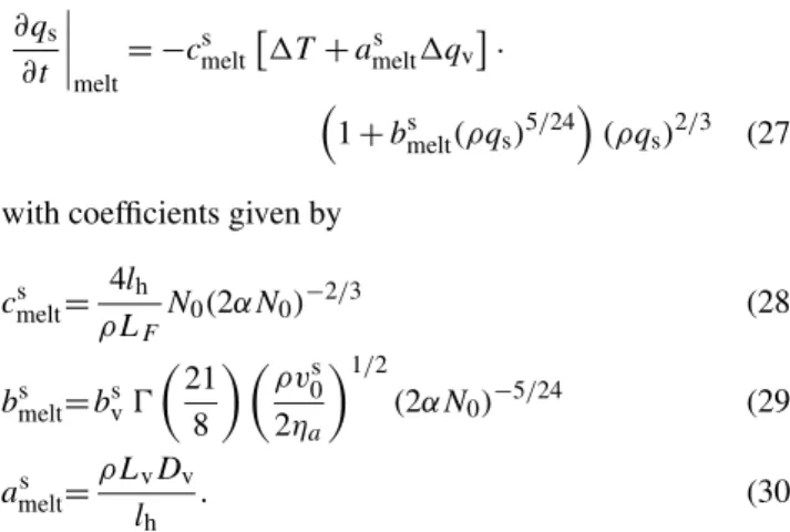
Table 1. The coefficients used within the Pade-type rational function (Eq. 34) for the melting integral and the conversion coefficient.
Ms
melt Msconv
ij pij qij pij qij
00 2.4436 1.0000 2.0163×10⁻¹ 1.0000
01 1.9817 3.1041×10⁻¹ −1.6515 1.5689×101
02 −1.3338×101 −2.499 2.6963 −1.6322
03 9.0218 1.2237 4.1582×10⁻¹ 1.2136
10 6.9311×10⁻¹ −9.4883×10⁻¹ 3.7192×10⁻¹ 2.1113
11 −1.7948 2.4705 1.6457×101 −1.5726×10⁻¹
12 1.1509 −6.1201×10⁻¹ −3.6523 −3.4157×10⁻¹
20 −1.5809 −2.5240×10⁻¹ 1.0552 2.7769
21 1.7492 −8.8062×10⁻¹ −1.0962×101 4.1566
30 1.3679×10⁻¹ 3.5516×10⁻¹ 1.2975 −3.0491
Table 2. The coefficients used within the Pade-type rational function (Eq. 34) for the two sedimentation velocities.
¯
vs,i v¯s,w
ij pij qij pij qij
00 1.2075 1.0000 1.0300 1.0000
01 −6.6499×10⁻¹ −1.0399 −4.0577×10⁻¹ −7.5945×10⁻¹ 02 −2.5636 −7.4739×10⁻¹ −2.5446 −6.1226×10⁻¹
03 2.3982 8.1807×10⁻¹ 2.7423 3.8234×10⁻¹
10 5.7709×10⁻¹ −2.8665×10⁻¹ 1.3996 −1.4119×10⁻¹ 11 −1.7521×10⁻¹ 3.6809×10⁻¹ −7.6087×10⁻¹ −5.9113×10⁻¹
12 −9.8016×10⁻² 2.8702×10⁻² 1.6117 1.1161
20 1.9702 1.3293 −1.5364 −3.6036×10⁻¹
21 −8.2445×10⁻¹ −1.2444 5.8759×10⁻² 2.8470×10⁻¹ 30 8.2598×10⁻⁴ 1.2643×10⁻⁴ −1.3725×10⁻³ −8.5578×10⁻⁵
To calculate the conversion from snow to rain the meltwa-ter within one time step is given by
smelt=cmelts [1T+amelts 1qv]Msmelt1t, (36) and is normalized with the ice mass mixing ratio of snow yielding the normalized melted water
ζ=smelt qs,i
. (37)
Note thatζ ∈ [0,1]. Given the snow ice mass mixing ratio at the current time stepqs,i(t )the value at the new time step, t+1t, is
qs,i(t+1t )=(1−ζ )qs,i(t ) (38)
andD∗(t+1t )as well asqs,w(t+1t )can in principle be calculated by increasingD∗until the ice mixing ratio of the distribution equalsqs,i(t+1t ). The conversion term is then given by
∂qs ∂t
conv
1t=Ms
conv[smelt+qs,w(t )] =Msconvqmelt (39)
with
Ms
conv=
smelt+qs,w(t )−qs,w(t+1t )
smelt+qs,w(t )
=qmelt−q (t+1t )
s,w qmelt
(40)
and hereqmeltis an intermediate value of the meltwater mix-ing ratio, i.e., after meltmix-ing but before the conversion to rain. Similar to the melting integral, this conversion coef-ficient Ms
conv, which is a function of ξ, L and ζ, can be pre-calculated numerically. Or in other words, by defining the normalized melt waterζ and calculating Ms
conv for all ζ ∈ [0,1]we avoid the expensive and cumbersome calcula-tion ofD∗(t+1t )andqs,w(t+1t ) during the runtime of the host model. Because of the normalization ofζ the dependency on ξ (or qs) is relatively weak and can be eliminated by aver-aging overξ. The resulting parametrization which is a func-tion of normalized meltwaterζ and bulk liquid water frac-tionLis shown in Fig. 3b and the corresponding coefficients
of Eq. (34) are presented in Table 1. The conversion coeffi-cient increases with the normalized melted waterζ, i.e., more meltwater is available for the conversion, and has the desir-able property thatMs
a) melting integral b) snow-rain conversion
c) sedimentation velocity of ice d) sedimentation velocity of melt water
Fig. 3.Parametrizations of(a)melting,(b)conversion, and the mass-weighted sedimentation velocities of(c)ice and(d)liquid mass. Here we have assumedms=αDs2withα=0.069 for the geometry of snow,̹=0.87 for the decay of the meltwater in the snow distribution, andN0= 8×10⁶m−4for the intercept parameter of the distribution of dry snow aloftfD=N0exp(−λDs). Shown are the analytic approximations using rational functions. The melting integral and the conversion coefficient are dimensionless quantities.
ice melts within the time step and all meltwater is immedi-ately transferred to rain.
In the atmosphere, lifted melting layers occur frequently, meaning that melting snow reaches an area with temperatures where it refreezes completely. For melting snow in an area of temperatures below−2◦C the meltwaterqs,wis therefore ascribed to the ice partqs,iwithin one time step.
The described parametrization is implemented into the COSMO model version 4.14. The new prognostic variable qs,w is included using a new generalized tracer implementa-tion in the COSMO model (Roches and Fuhrer, 2012). For both mixing ratios,qs,wandqs,i, the same advection scheme is applied. As initial and boundary conditions for the new prognostic meltwater we useqs,w=0 since this variable is not yet implemented in the data assimilation system and the large-scale models that provide the boundary conditions.
3 First results
Fig. 4. ECMWF analysis fields at 12:00 UTC, 16 November 2010. Shown is sea-level pressure (black contours, every 2 hPa) and po-tential temperature at 850 hPa (colours, in K). The black dot marks Dresden and the black rectangle the area shown in Fig. 5.
from dry snow to melting snow to rain, (iii) leads to a decel-erated snow melting process, and (iv) can provide novel and useful forecast information in situations of wet surface snow-fall. An in-depth validation of the new snow melting scheme, based upon re-forecasts of a large set of situations, is beyond the scope of this study.
3.1 Simulation of a snow melting layer on 16 November 2010
The first event on 16 November 2010 featured snowfall in eastern Germany in a region with surface temperatures in the range of±5◦C. The synoptic situation over Central Eu-rope at 12:00 UTC, 16 November 2010 was characterised by a pronounced upper-level trough, extending from the North Sea into the Mediterranean (not shown). The surface pressure field features a persistent high-pressure system over south-ern Scandinavia and an intense cyclone in the Gulf of Genoa (Fig. 4). Potential temperature at 850 hPa shows relatively cold air over France and Germany and a prominent frontal zone extending along the border between Germany and the Czech Republic and across Poland. It is along this frontal zone that the snow melting event occurred. Surface observa-tions in Dresden (black dot in Fig. 4) indicate a 2 m temper-ature of 5.1◦C and 98 % relative humidity with continuous (moderate) rain at 12:00 UTC and light drizzle at 14:00 UTC. Additionally, radar observations in Dresden (not shown) pro-vide epro-vidence for precipitation in the frontal area and show an enhanced radar reflectivity indicating the likely occurrence of melting hydrometeors.
Results shown here are from a simulation started at 12:00 UTC, 16 November 2010, i.e., just two hours prior to the time of the analysis of the snow melting event in eastern
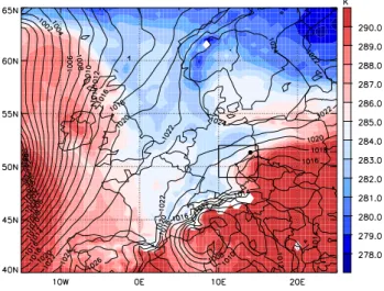
Germany. Such a short simulation has been chosen in or-der to minimise the feedback of the modified microphysical scheme on the dynamics of the event, which would render a comparison of the performance of the two schemes more difficult. We note however that earlier simulations started at 00:00 and 06:00 UTC, 16 November 2010 reveal quali-tatively similar results. At 14:00 UTC (Fig. 5), the horizontal section on model level 8 (about 920 hPa) shows a west-east oriented band of cold air with temperatures below 0◦C (see green contour) in eastern Germany. Both simulations pro-duce snow in this area, but the simulation with the standard melting scheme produces less snow in the region to the north of the cold band (i.e., in an area with temperatures larger than 0◦C) compared to the simulation with the new melt-ing scheme (compare Fig. 5a and b). The increased snow in this region mainly consists of partially melted snow as indi-cated by the snow meltwater mixing ratio shown by the red contours in Fig. 5b.
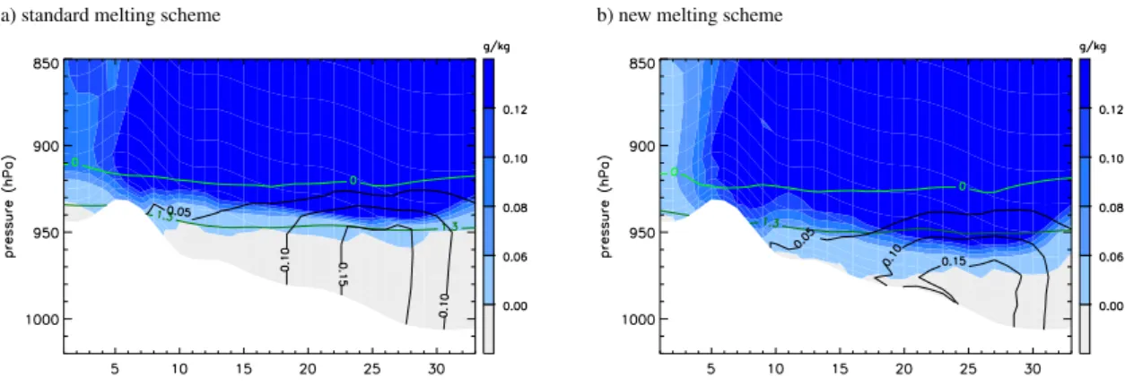
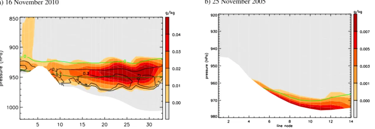
Vertical sections across the snow band, i.e., along the black lines shown in Fig. 5, clearly show the decelerated snow melting process due to the new parametrization (Fig. 6). The green line represents the 0◦C isoline, which marks ap-proximately the top of the melting layer. For the bottom of the melting layer the isoline of 1.3◦C wet bulb tempera-ture (dark green lines) appears to be a reasonable indicator. With the new scheme, snow penetrates to slightly lower lev-els (slightly below the 1.3◦C contour of wet bulb tempera-ture) and, consistently, the rain contours are shifted to lower altitudes (compare Fig. 6a and b). The simulated meltwater in the simulation with the new melting scheme (Fig. 7a) indi-cates a qualitatively realistic representation of the snow melt-ing process. The simulated meltmelt-ing layer has a vertical exten-sion of about 40 hPa and is approximately sandwiched be-tween the contours of 0◦C temperature and 1.3◦C wet bulb temperature. Of course, such a melting layer characterised by a transition from dry snow to wet snow to rain cannot be represented by the standard snow melting scheme. The verti-cal resolution of the presented COSMO simulations provides about 10 levels in the lowest 100 hPa. Therefore, the investi-gated melting layer extends over approximately 4 model lev-els.
a) standard melting scheme b) new melting scheme
Fig. 5. Snow mixing ratio (colours, in g kg−1), meltwater mixing ratio (red contours, in g kg−1, only in panelb), and the 0◦C isoline (green contour) on model level 8 at 14:00 UTC, 16 November 2010 for the simulations with(a)the standard and(b)the new snow melting scheme. The dashed box marks the main area of interest while the black line indicates the location of the vertical cross sections shown in Figs. 6 and 7a.
a) standard melting scheme b) new melting scheme
Fig. 6. Vertical section across the snowfall region in eastern Germany at 14:00 UTC, 16 November 2010 (along the black line shown in Fig. 5). Shown are snow mixing ratio (colours, in g kg−1), rain mixing ratio (black lines, in g kg−1), the 0◦C temperature isoline (green), and the isoline of 1.3◦C wet bulb temperature (dark green) for the simulations with(a)the standard and(b)the new snow melting scheme.
to decrease, while the liquid water fraction of the snow still increases due to ongoing melting.
3.2 Simulation of wet surface snowfall on 25 November 2005
COSMO hindcast simulations for the wet snowfall event in northwestern Germany in November 2005 have been de-scribed by Frick and Wernli (2012). They showed that in the area affected by wet snow short-range COSMO hind-casts with the standard snow melting scheme produce a large amount of surface precipitation in liquid form (about 50 %) even when capturing the low-tropospheric temperature struc-ture fairly accurately. Here one of these hindcast simulations, initialised at 12:00 UTC, 24 November, is repeated with the new snow melting scheme. Figure 8 shows the snow mixing ratio on the lowest model level at 03:00 UTC, 25 Novem-ber for both simulations with the standard and the new melt-ing scheme, respectively. It is at this time that wet snowfall
started at the monitoring station in Essen (Frick and Wernli, 2012). The overall distribution is fairly similar (compare Fig. 8a and b), but the domain integrated snow fraction, i.e., the ratio from surface snowfall to total precipitation, is in-creased by a few percents. In a fairly large area in Belgium, the Netherlands and western Germany, in a band of about 100 km to the north of the 0◦C isotherm, snow reaches the surface with a significant meltwater mixing ratio (see red contours in Fig. 8b), i.e., as wet snow. This is also revealed by the vertical section across the area with strongest (wet) sur-face snowfall (Fig. 7b), which shows the formation of a layer with non-zero meltwater mixing ratio in the simulation with the new snow melting scheme, extending from the freezing level down to the surface.
3.3 Statistical analysis of the snow fraction
a) 16 November 2010 b) 25 November 2005
Fig. 7. Vertical cross sections from simulations with the new snow melting scheme of the meltwater mixing ratio (colours, in g kg−1). Panel (a)shows the same section as Fig. 6 at 14:00 UTC, 16 November 2010. Also shown are the liquid water fraction (black contours for values of 0.2, 0.3 and 0.4), the 0◦C isoline of temperature (green contour), and the isoline of 1.3◦C wet bulb temperature (dark green contour). Panel (b)shows a section across the wet snowfall area (see black line in Fig. 8) at 03:00 UTC, 25 November 2005.
a) standard melting scheme b) new melting scheme
Fig. 8. Snow mixing ratio (colours, in g kg−1), meltwater mixing ratio (red contours for 2, 6, 8, 10 mg kg−1, only in panelb), and the 0◦C isoline (green contour) on model level 1 at 03:00 UTC, 25 November 2005 for the simulations with(a)the standard and(b)the new snow melting scheme. The black line indicates the location of the vertical cross section shown in Fig. 7b.
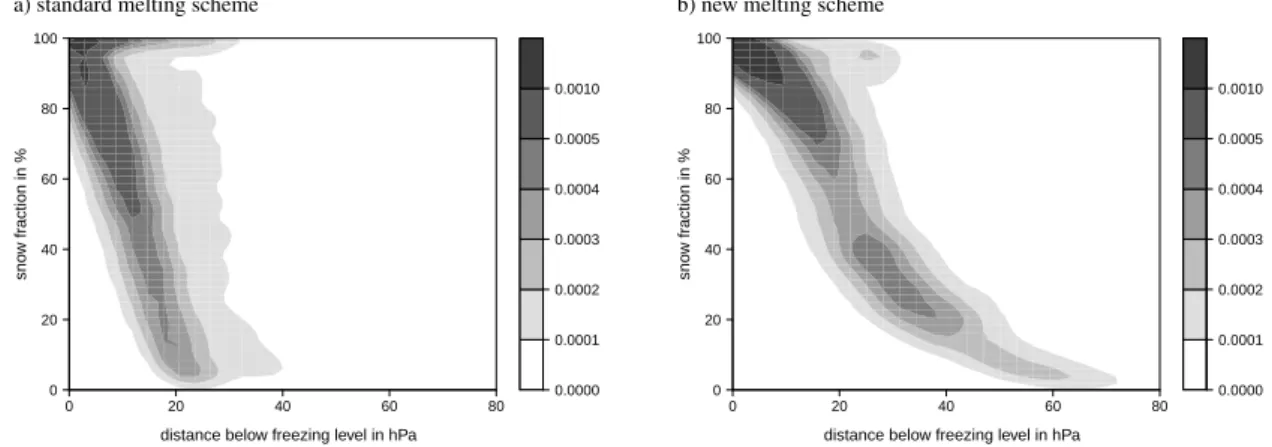
has been performed for the snowfall event discussed in Sect. 3.1, initialized at 00:00 UTC, 16 November 2010. This simulation has been chosen in order to capture the entire snowfall that occurred during this day. The simulated precip-itation is investigated in the main snowfall region indicated by the dashed box in Fig. 5. For each gridpont in this area associated with a snow mixing ratio larger than zero and a temperature above 0◦C the ratio of snow to total precipita-tion (snow fracprecipita-tion,qs/ (qs+qr)) and the distance to the top
of the melting layer (i.e., the 0◦C isosurface) are calculated. The resulting relations for the standard and the new melt-ing scheme are presented in Fig. 9. As expected both schemes show a decreasing snow fraction with increasing distance below the top of the melting layer. However, the slope of the relation is much steeper for the standard scheme, which indicates a more rapid conversion from snow to rain. Note that the relatively large scatter of the relation is due to the
variability of humidity, precipitation intensity, and advec-tion of precipitaadvec-tion at the different grid points. 20 hPa below the top of the melting level the standard scheme reduces the snow fraction to typically less than 20 %, while with the new scheme still about half of the hydrometeors correspond to (partially melted) snow. In regions where this altitude corre-sponds to the surface, the two schemes produce a strikingly different surface precipitation signal with hardly any snow (standard scheme) versus much larger amounts of potentially heavy wet snow (new scheme).
a) standard melting scheme
0.0000 0.0001 0.0002 0.0003 0.0004 0.0005 0.0010
0 20 40 60 80
0 20 40 60 80 100
sno
w fr
action in %
distance below freezing level in hPa
b) new melting scheme
0.0000 0.0001 0.0002 0.0003 0.0004 0.0005 0.0010
0 20 40 60 80
0 20 40 60 80 100
sno
w fr
action in %
distance below freezing level in hPa
Fig. 9. The frequency distribution of the ratio of snow to overall precipitation (snow fraction) for all gridpoints with snow and temperatures above 0◦C as a function of the vertical distance below the top of the melting layer,(a)for the standard and(b)the new snow melting scheme. Results are from a November 2010 hindcast simulation (see text).
the intercept parameterD∗is already that large and the snow mixing ratioqsthat small due to snow to rain conversion that the ensemble mainly consists of few large snowflakes that melt relatively slowly.
In general, the melting rate is reduced by the new melting scheme. This finding is also supported by the evolution of the ice fraction (qs,i/ (qs+qr), not shown) which has a slightly
more compact density distribution but a slope comparable to the one of the snow fraction.
This statistical analysis indicates that the melting process is decelerated by the new parametrization and snow is able to reach much farther below the top of the melting layer (up to 70 hPa compared to 30 hPa with the standard scheme).
4 Conclusions
A new snowflake melting scheme has been introduced and implemented into the COSMO model version 4.14. The source code is available from the authors1and it is intended to include the new scheme in later versions of the official COSMO code. The new melting parametrization allows the explicit prediction of partially melted snow (i.e., wet snow) using a prognostic meltwater mixing ratio. The formulations of capacitance, ventilation coefficient and fall velocity of a single melting snowflake follow mainly the empirical and theoretical findings of M90. For an ensemble of snowflakes, as described by the COSMO model, flux conservation is used to determine the size distribution of melting snowflakes. A size resolved liquid water fraction is defined following SZ99 and the meltwater and ice part of snow are treated as separate parameters. The parametrization is implemented by using ap-proximations in form of rational functions for the hydrome-teor fall velocities, the melting integral, and the conversion rate from snow to rain.
1Co-authors: [email protected], [email protected]
First case studies of snowfall events associated with a melting layer illustrate the potential of the new snow melt-ing scheme. Hindcast simulations with the new scheme of a frontal snowfall event in eastern Germany in November 2010 produce a melting layer with semi-melted snow particles in the lower troposphere with a vertical extension of about 40 hPa. The meltwater fraction attains peak values of about 0.3 at the bottom of the melting layer. In contrast, the peak of the meltwater mixing ratio is reached at a slightly higher alti-tude. Qualitatively, this simulated melting layer corresponds nicely to the “bright band” as observed by radar. At the sur-face, wet snow is predicted in fairly large areas with surface temperatures above 0◦C and, compared to the simulation with the standard scheme, the total area of surface snow-fall is substantially larger. This indicates that with the new scheme, the snow melting process in the atmosphere is de-celerated and the snow particles reach to lower levels com-pared to the standard scheme. The second case study of the high-impact wet snowfall event in northwestern Germany in November 2005 (Frick and Wernli, 2012) shows a clear qual-itative improvement of the simulation of the surface precipi-tation type when using the new snow melting scheme. With the new scheme, semi-melted snow is simulated at the sur-face in regions where wet snowfall was observed and simu-lations with the standard scheme produced surface rainfall.
Acknowledgements. We thank S. K. Mitra (University of Mainz) for providing the original data of Mitra et al. (1990), which is shown in Fig. 1d. Anne Roches (C2SM, ETH Zurich) and Oliver Fuhrer (MeteoSwiss) are acknowledged for their help with implementing the new COSMO model tracer algorithm and MeteoSwiss for providing access to the ECMWF analysis data. We also thank the two anonymous reviewers for their detailed and constructive comments, which helped to improve the presentation of our approach.
Edited by: V. Grewe
References
Austin, P. M. and Bemis, A. C.: A quantitative study of the “bright band” in radar precipitation echoes, J. Meteor., 7, 145–151, 1950. Barthazy, E., Waldvogel, A., Urban, U., and Randeu, W.: Melt dis-tances of snowflakes, Preprints, Conf. on Cloud Physics, Amer. Met. Soc., 140–141, 1998.
Berry, E. X. and Reinhardt, R. L.: An analysis of cloud drop growth by collection: Part I. Double distributions, J. Atmos. Sci., 31, 1814–1824, 1974.
Bocchieri, J. R.: The objective use of upper air soundings to specify precipitation type, Mon. Weather Rev., 108, 596–603, 1980. Brandes, E. A., Ikeda, K., Zhang, G., Schönhuber, M., and
Ras-mussen, R. M.: A statistical and physical description of hydrom-eteor distributions in Colorado snowstorms using a video dis-drometer, J. Appl. Meteor., 46, 634–650, 2007.
Braun, S. A. and Houze: Melting and freezing in a mesoscale con-vective system, Quart. J. Roy. Met. Soc., 121, 55–77, 1995. Cotton, W. R., Tripoli, G. J., Rauber, R. M., and Mulvihill, E. A.:
Numerical simulation of the effects of varying ice crystal nu-cleation rates and aggregation processes on orographic snowfall, J. Clim. Appl. Met., 25, 1658–1680, 1986.
Czys, R. R., Scott, R. W., Tang, K. C., Przybylinski, R. W., and Sabones, M. E.: A physically based, nondimensional parameter for discriminating between locations of freezing rain and sleet, Weather Forecast., 11, 591–598, 1996.
Doms, G. and Schättler, U.: A description of the nonhydrostatic re-gional Mmdel LM, Part I: Dynamics and numerics, Offenbach, Germany, 2002.
Fabry, F. and Szyrmer, W.: Modeling of the Melting Layer. Part II: Electromagnetic, J. Atmos. Sci., 56, 3593–3600, 1999.
Fabry, F. and Zawadzki, I.: Long-term radar observations of the melting layer of precipitation and their interpretation, J. At-mos. Sci., 52, 838–851, 1995.
Ferrier, B. S.: A double-moment multiple-phase four-class bulk ice scheme. Part I: Description, J. Atmos. Sci., 51, 249–280, 1994. Field, P., Hogan, R., Brown, P., Illingworth, A., Choularton, T.,
and Cotton, R.: Parametrization of ice-particle size distributions for mid-latitude stratiform cloud, Quart. J. Roy. Met. Soc., 131, 1997–2017, 2005.
Field, P. R., Heymsfield, J., Bansemer, A., and Twohy, C. H.: Deter-mination of the combined ventilation factor and capacitance for ice crystal aggregates from airborne observations in a tropical anvil cloud, J. Atmos. Sci., 65, 376–391, 2008.
Frick, C. and Wernli, H.: A case study of high-impact snowfall in NW Germany (25–27 Nov 2005): Observations, dynamics and forecast performace, Weather Forecast., 27, 1217–1234, 2012.
Fujiyoshi, Y.: Melting snowflakes, J. Atmos. Sci., 43, 307–311, 1986.
Gunn, K. and Marshall, J.: The distribution with size of aggregate snowflakes, J. Appl. Met., 15, 452–461, 1958.
Hall, W. D. and Pruppacher, H. R.: The survival of ice particles falling from cirrus clouds in subsaturated air, J. Atmos. Sci., 33, 1995–2006, 1976.
Khvorostyanov, V. and Curry, J.: Terminal velocities of droplets and crystals: Power laws with continuous parameters over the size spectrum, J. Atmos. Sci., 59, 1872–1884, 2002.
Khvorostyanov, V. and Curry, J.: Fall velocities of hydrometeors in the atmosphere: Refinements to a continuous analytical power law, J. Atmos. Sci., 62, 4343–4357, 2005.
Knight, C. A.: Observations of the morphology of melting snow, J. Atmos. Sci., 36, 1123–1132, 1979.
Lim, K.-S. S. and Hong, S.-Y.: Development of an effective double-moment cloud microphysics scheme with prognostic cloud condensation nuclei (CCN) for weather and climate mod-els, Mon. Weather Rev., 138, 1587–1612, 2010.
Lin, C. A. and Stewart, R. E.: Mesoscale circulations initiated by melting snow, J. Geophys. Res., 91, 299–302, 1986.
Lin, Y.-L., Farley, R. D., and Orville, H.: Bulk parametrization of the snow field in a cloud model, J. Clim. Appl. Meteorol., 22, 1065–1092, 1983.
Matsuo, T. and Sasyo, Y.: Melting of snowflakes below freezing level in the atmosphere, J. Meteor. Soc. Japan, 59, 10–25, 1981. Meyers, M. P., Walko, R. L., Harrington, J. Y., and Cotton, W. R.:
New RAMS cloud microphysics parametrization. Part II: The two-moment scheme, Atmos. Res., 45, 3–39, 1997.
Mitra, S. K., Vohl, O., Ahr, M., and Pruppacher, H. R.: A wind tun-nel and theoretical study of the melting behaviour of atmospheric ice particles. IV: Experiment and theory for snow flakes, J. At-mos. Sci., 47, 584–591, 1990.
Mölders, N., Laube, M., and Kramm, G.: On the parametrization of ice microphysics in a mesoscalealphaweather forecast model, Atmos. Res., 38, 207–235, 1995.
Morrison, H., Curry, J., and Khvorostyanov, V.: A new double-moment microphysics parametrization for application in cloud and climate models. Part I: Description, J. Atmos. Sci., 62, 1665– 1677, 2005.
Phillips, V. T. J., Pokrovsky, A., and Khain, A.: The influence of time-dependent melting on the dynamics and precipitation pro-duction in maritime and continental storm clouds, J. Atmos. Sci., 64, 338–359, 2007.
Press, W. H., Teukolsky, S. A., Vetterling, W. T., and Flannery, B. P.: Numerical recipes in FORTRAN, Cambridge University Press, Cambridge, 1992.
Pruppacher, H. R. and Klett, J. D.: Microphysics of clouds and pre-cipitation, Kluwer Academic Publishers, Dordrecht, 1997. Raga, G. B., Stewart, R. E., and Donaldson, N. R.: Microphysical
characteristics through the melting region of a midlatitude winter storm, J. Atmos. Sci., 48, 843–855, 1991.
Rauber, R. M., Olthoff, L. S., Ramamurthy, M. K., and Kunkel, K. E.: Further investigation of a physically based, nondimen-sional parameter for discriminating between locations of freez-ing rain and ice pellets, Weather and Forecastfreez-ing, 16, 185–191, 2001.
MM5 mesoscale model, Quart. J. Roy. Met. Soc., 124, 1071– 1107, 1998.
Roches, A. and Fuhrer, O.: Tracer module in the COSMO model, Consortium for Small-Scale Modelling. Technical report No. 20, 2012.
Rutledge, S. A. and Hobbs, P. V.: The mesoscale and microscale structure and organization of clouds and precipitation in midlati-tude cyclones XII: A diagnostic modeling study of precipitation development in narrow cold-frontal rainbands, J. Atmos. Sci., 41, 2949–2972, 1984.
Seifert, A. and Beheng, K.: A two-moment cloud microphysics parametrization for mixed-phase clouds. Part I: Model Descrip-tion, Meteorol. Atmos. Phys., 92, 45–66, 2006.
Szyrmer, W. and Zawadzki, I.: Modeling of the melting layer. Part I: Dynamics and Microphysics, J. Atmos. Sci., 56, 3573–3592, 1999.
Szyrmer, W. and Zawadzki, I.: Snow studies. Part II: Average rela-tionship between mass of snowflakes and their terminal fall ve-locity, J. Atmos. Sci., 67, 3319–3335, 2010.
Thériault, J. M., Steward, R. E., Milbrandt, J. A., and Yau, M. K.: On the simulation of winter precipitation types, J. Geophys. Res., 111, doi:10.1029/2005JD006665, 2006.
Thompson, G., Field, P. R., Rasmussen, R. M., and Hall, W. D.: Ex-plicit forecasts of winter precipitation using an improved bulk microphysics scheme. part ii: implementation of a new snow parametrization, Mon. Weather Rev., 136, 5095–5115, 2008.
Walko, R. L., Cotton, W. R., Meyers, M. P., and Harrington, J. Y.: New RAMS cloud microphysics parametrization. Part I: The single-moment scheme, Atmos. Res., 38, 29–62, 1995.
Westbrook, C., Ball, R., Field, P., and Heymsfield, A.: Uni-versality in snowflake aggregation, Geophys. Res. Lett., 31, doi:10.1029/2004GL020363, 2004a.
Westbrook, C., Ball, R., Field, P., and Heymsfield, A.: Theory of growth by differential sedimentation, with application to snowflake formation, Phys. Rev. E, 70, doi:10.1103/PhysRevE.70.021403, 2004b.
Willis, P. T. and Heymsfield, A. J.: Structure of the melting layer in mesoscale convective system stratiform precipitation, J. At-mos. Sci., 46, 2008–2025, 1989.
Wilson, D. R. and Ballard, S. P.: A microphysically based pre-cipitation for the UK Meteorological Office Unified Model, Quart. J. Roy. Met. Soc., 125, 1607–1636, 1999.
Woods, C. P., Stoelinga, M. T., and Locatelli, J. D.: The improve-1 storm of 1–2 february 2001. part III: Sensitivity of a mesoscale model simulation to the representation of snow particle types and testing of a bulk microphysical scheme with snow habit predic-tion, J. Atmos. Sci., 64, 3927–3948, 2007.