INVESTIGATIONS ON THINNING
AND THICKENING LINEAR ARRAYS
U.V. RATNA KUMARI
Assistant Professor, Department of Electronics and Communication Engineering, University College of Engineering Kakinada, JNTUK Kakinada.
Dr. G.M.V. PRASAD
Principal, BVCITS, Amalapuram, Andhra Pradesh, India [email protected]
Dr. G.S.N. RAJU
Professor, Department of Electronics and Communication Engineering, College of Engineering, Andhra University, Visakhapatnam, Andhra Pradesh, India
Abstract
Array antennas are preferred over discrete antennas to obtain the specified directivity, gain and radiation patterns. The radiation patterns are controlled by different parameters which include amplitude and phase of the excitations, positioning the elements in the array, and the type of the elements. Although some studies are made by the researchers on thinning, the effect of thickening is not reported in the literature. Moreover, the effects for gradual thinning and gradual thickening are not available.
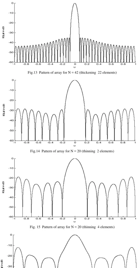
In view of the above facts, intensive studies are carried out to investigate linear arrays with gradual thickening as well as gradual thinning. The patterns are numerically evaluated for different arrays and the radiation patterns are presented for different arrays. The investigations reveal that thickening has caused the reduction of null to null beam width without deteriorating the side lobe levels. On the other hand thinning has resulted in raising the side lobe levels as well as the beam width. If thinning is not carried out properly the resultant radiation patterns contain even grating lobes.
Keywords: Array antenna, thinning, thickening, radiation pattern 1. Introduction
Discrete radiating elements are characterized by multidirectional radiation patterns. Most often their gain and directivity are inadequate. In order to meet the requirements of above parameters, array antennas are preferred. Arrays are of different types [1,2]. In the present work uniformly spaced linear arrays are considered, to generate radiation patterns with cost effectiveness.
Taylor’s method of distribution [3] is used as the basis. Different arrays are considered and the method of thinning and thickening are employed. Comparative studies are made on the radiation patterns. In fact patterns are generated by many methods. Schelkunoff polynomial method [4] generates a pattern with the nulls in specified directions. For the design of the array, the number of nulls and their locations are specified. The number of radiating elements and their excitation levels can be obtained as the nulls and their locations are known. Using Fourier transform method the excitation distribution of either a continuous line source or a discrete array for a specified radiation pattern can be designed.
Woodward Lawson method [5,6] consists of sampling the desired pattern and the locations. Therefore the excitation function for a continuous line source and the excitation levels for a discrete array are found. This method is used for beam shaping. But there is no control over the side lobe levels in the trade off region of the pattern. Dolph Tchebyscheff method [7] is used to determine the suitable polynomials which give the excitation coefficients to obtain the patterns between uniform and binomial arrays. This gives a radiation pattern containing one main beam and side lobes, with the same level by finding the spacing of nulls.
Taylor’s method of amplitude distribution gives a pattern which exhibits an optimum compromise between beam width and side lobe levels. Taylor’s patterns contain a specified number of side lobes close to the main lobe at equal level and the remaining side lobes decrease monotonically. This decay is a function of space over which these side lobes are required to be at the same level.
gradual thinning is adopted. The respective radiation patterns are numerically computed. The method of thickening is also used in the present work and the radiation patterns of the resultant arrays are evaluated.
2. Formulation
The procedure for designing continuous line sources has been described by Taylor. The expression for radiation pattern as given by Taylor, is
n 1
1 n 2 2 2 2 2 2 2 n u 1 2 1 n A u 1 u u sin A cosh ) u (
E (1)
Where is an integer which divides the radiation pattern into uniform sidelobe region surrounding the main beam and the region of decaying sidelobes.
u= sin
= Length of the array
= angle measured from the direction of maximum radiation
A is an adjustable real parameter having the property that coshπA is the side lobe ratio
σ =
From the above expression (1), the aperture distribution of the array is found by applying Woodward’s method [5]. The aperture field distribution A(x) may be expressed as
n x jn ne a ) x (A (2)
Where x = z/L ( z being the variable point on the aperture) The pattern E(u) is related to A(x) by the expression
1 1 jux dx e ) x ( A ) u (E (3)
From equations (2) and (3) we get
1 n n n u n u sin a ) u ( E (4) This givesE(u) │u = nπ (5)
Hence expression for E(u) reduces to
1n u n
n u sin ) n ( E ) u (
E (6)
The aperture function may be expressed as
1 n n0 2a cosn x
a ) x ( A
1 n ) x n ( cos ) n ( E 2 ) 0 ( E (7)E(n = 0 for n
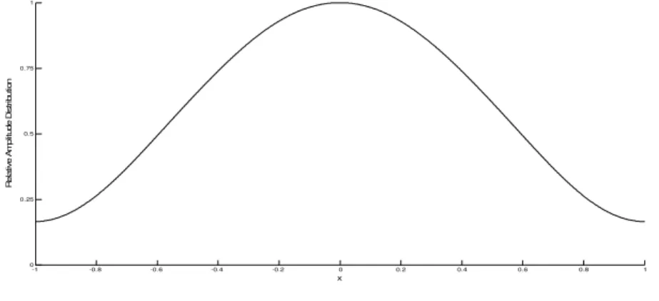
Using the above expressions (1) and (7) the aperture distribution of the array having side lobe ratio equal to -35 dB and equal to 6 is computed and the results (normalized values) are presented.
3. Results
Using the expression (7) the amplitude distribution across the continuous line source for a sidelobe level of -35dB and = 6 is numerically computed and it is presented in fig. 1. The amplitude distribution so obtained is discretized and the excitation levels for each radiating element of an array are found out. Using these levels the radiation pattern are computed for gradually thinned and thickened arrays. Results are presented in figures (2- 16). The variation of beamwidth and side-lobe levels for the above arrays is considered and presented in tables (1 – 2).
-1 -0.8 -0.6 -0.4 -0.2 0 0.2 0.4 0.6 0.8 1
0 0.25 0.5 0.75 1
x
R
e
la
tiv
e
A
m
p
lit
ud
e D
is
tr
ibu
tion
Fig. 1 Talylor Amplitude Distribution for SLL= -35 dB and n = 6
-1 -0.8 -0.6 -0.4 -0.2 0 0.2 0.4 0.6 0.8 1 -60
-50 -40 -30 -20 -10 0
u
IE
(u
)I
i
n
d
B
Fig.2 Pattern of array for N = 20
-1 -0.8 -0.6 -0.4 -0.2 0 0.2 0.4 0.6 0.8 1 -60
-50 -40 -30 -20 -10 0
u
IE
(u
)I
in
d
B
-1 -0.8 -0.6 -0.4 -0.2 0 0.2 0.4 0.6 0.8 1 -60
-50 -40 -30 -20 -10 0
u
IE
(u
)I
i
n
d
B
Fig.4 Pattern of array for N = 24 (thickening 4 elements)
-1 -0.8 -0.6 -0.4 -0.2 0 0.2 0.4 0.6 0.8 1 -60
-50 -40 -30 -20 -10 0
u
IE
(u
)I
i
n
d
B
Fig.5 Pattern of array for N = 26 (thickening 6 elements)
-1 -0.8 -0.6 -0.4 -0.2 0 0.2 0.4 0.6 0.8 1 -60
-50 -40 -30 -20 -10 0
u
IE
(u
)I
i
n
d
B
-1 -0.8 -0.6 -0.4 -0.2 0 0.2 0.4 0.6 0.8 1 -60
-50 -40 -30 -20 -10 0
u
IE
(u
)I
i
n
d
B
Fig.7 Pattern of array for N = 30 (thickening 10 elements)
-1 -0.8 -0.6 -0.4 -0.2 0 0.2 0.4 0.6 0.8 1 -60
-50 -40 -30 -20 -10 0
u
IE
(u
)I
in
d
B
Fig.8 Pattern of array for N = 32 (thickening 12 elements)
-1 -0.8 -0.6 -0.4 -0.2 0 0.2 0.4 0.6 0.8 1 -60
-50 -40 -30 -20 -10 0
u
IE
(u
)I
in
d
B
-1 -0.8 -0.6 -0.4 -0.2 0 0.2 0.4 0.6 0.8 1 -60
-50 -40 -30 -20 -10 0
u
IE
(u
)I
i
n
d
B
Fig.10 Pattern of array for N = 36 (thickening 16 elements)
-1 -0.8 -0.6 -0.4 -0.2 0 0.2 0.4 0.6 0.8 1 -60
-50 -40 -30 -20 -10 0
u
IE
(u
)I
in
d
B
Fig.11 Pattern of array for N = 38 (thickening 18 elements)
-1 -0.8 -0.6 -0.4 -0.2 0 0.2 0.4 0.6 0.8 1 -60
-50 -40 -30 -20 -10 0
u
IE
(u
)I
in
d
B
-1 -0.8 -0.6 -0.4 -0.2 0 0.2 0.4 0.6 0.8 1 -60
-50 -40 -30 -20 -10 0
u
IE
(u
)I
i
n
d
B
Fig.13 Pattern of array for N = 42 (thickening 22 elements)
-1 -0.8 -0.6 -0.4 -0.2 0 0.2 0.4 0.6 0.8 1
-60 -50 -40 -30 -20 -10 0
u
IE
(u
)I
i
n
d
B
Fig.14 Pattern of array for N = 20 (thinning 2 elements)
-1 -0.8 -0.6 -0.4 -0.2 0 0.2 0.4 0.6 0.8 1
-60 -50 -40 -30 -20 -10 0
u
IE
(u
)I
i
n
d
B
Fig. 15 Pattern of array for N = 20 (thinning 4 elements)
-1 -0.8 -0.6 -0.4 -0.2 0 0.2 0.4 0.6 0.8 1
-60 -50 -40 -30 -20 -10 0
u
IE
(u
)I
in
d
B
Table1: Beam width and SLL for Thinning of Linear Array
Sl.no. Number of elements First Side Lobe Level
(SLL) in dB Beam Width
1 20 -35.17 0.3012
2 18 -28.03 0.3420
3 16 -23.27 0.4088
4 14 -22.36 0.5872
5 12 -14.71 0.3396
6 10 -20.31 0.2756
Table2: Beam width and SLL for Thickening of Linear Array
Sl.no. Number of elements First Side Lobe Level
(SLL) in dB Beam Width
1 22 -35.12 0.3012
2 24 -35.15 0.2762
3 26 -35.17 0.2552
4 28 -35.17 0.239
5 30 -35.17 0.2212
6 32 -35.16 0.2092
7 34 -35.16 0.19522
8 36 -35.16 0.18434
9 38 -35.17 0.17466
10 40 -35.17 0.16736
11 42 -35.32 0.158
12 44 -35.31 0.15212
13 46 -35.19 0.1441
14 48 -35.19 0.13828
15 50 -35.19 0.1339
16 52 -35.19 0.12874
17 54 -35.19 0.12294
18 56 -35.19 0.11852
19 58 -35.19 0.11446
20 60 -35.19 0.11064
21 62 -35.19 0.10712
22 64 -35.19 0.10374
23 66 -35.19 0.10058
24 68 -35.19 0.09848
25 70 -35.19 0.09484
26 72 -35.19 0.093
27 74 -35.19 0.08966
28 76 -35.19 0.0881
29 78 -35.19 0.08544
30 80 -35.19 0.08302
4. Conclusions
References
[1] G.S.N. Raju, “Antennas and Wave Propagation”, Pearson Education (Singapore) Pte. Ltd, 2005.
[2] R.S Elliot, “Antenna Theory and Design” printice-hall, New York, 1981.
[3] T.T.Taylor, “Design of Line Source Antennas for Narrow Beamwidth and Low Sidelobes,” IRE Trans. Antennas and Propagation
AP-3(1955)
[4] S.A.Schelkunoff, ”A Mathematical Theory of Linear Arrays,” Bell System Tech., J., Vol. 22(1943)
[5] P.M.Woodward, ”A Metod of Calculating the Field over a Plane Aperture Required to Produce a Given Polar Diagram,”
J.IEEE(London), Pt. IIIA ,93(1946)
[6] P.M.Woodward and J.D.Lawson , “The Theoretical Precision with Which an Arbitrary Radiation May be Obtained from a Source of
Finite Extent,“ J.IEE, Vol 95, part II(1948)
[7] C.L.Dolph, “ A Current Distribution for Broadside Arrays Which Optimises the Relationship between Beam Width and Side-Lobe