Brazilian Microwave and Optoelectronics Society-SBMO received 23 Feb 2017; for review 02 Mar 2017; accepted 14 May 2017 Abstract—This paper presents the optimization performance of non-uniform linear antenna array with optimized inter-element spacing and excitation amplitude using Particle Swarm Optimization (PSO). The aim of the proposed algorithm is to obtain the optimum values for inter-element spacing and excitation amplitude for a linear antenna array in a given radiation pattern with suppressed Side Lobe Level (SLL), minimum Half Power Beamwidth (HPBW), improved directivity and placement of nulls in the desired direction. A variety of design examples are considered and the obtained results using PSO are validated by benchmarking with results obtained using other nature-inspired meta-heuristic algorithms such as the Real-coded Genetic Algorithm (RGA) and the Biogeographic Based Optimization (BBO) algorithm. The comparative results are shown that optimization of linear antenna array using the PSO provides considerable enhancement in the SLL, the HPBW, the directivity and the null control in the desired direction.
Index Terms—Linear Antenna Array, Improved Directivity, Null Control, Particle Swarm Optimization, Minimum Side Lobe Level, Half Power Beamwidth.
I. INTRODUCTION
An antenna array is a combination of two or more antenna elements that can be placed in a specific geometry. In a linear antenna array, antenna elements are placed along one axis. The antenna array produces a beam, this beam can effect by changing the geometry (linear, circular, spherical etc.) and also by some other parameters i.e. inter-element spacing, excitation amplitude and excitation phase of the individual element [1]. In mostly wireless communication requires more directive antenna having high gain. Antenna array has high gain, more directive, spatial diversity. Antenna array synthesis has received importance in the near past, where various performance goals were considered. For array synthesis, different optimization algorithms e.g., the simulated annealing [2], the ant-colony
Analysis of Linear Antenna Array for
minimum Side Lobe Level, Half Power
Beamwidth, and Nulls control using PSO
Saeed Ur Rahman¹, Qunsheng CAO¹, 1College of Electronics and Information Engineering, Nanjing University of Aeronautics and Astronautics (NUAA),
Nanjing 2111016, China
[email protected] , [email protected]
Muhammad Mansoor Ahmed², Hisham Khalil² 2
Department of Electrical Engineering,
Brazilian Microwave and Optoelectronics Society-SBMO received 23 Feb 2017; for review 02 Mar 2017; accepted 14 May 2017
optimization [3], the GA [4] and the PSO [5] have been used in the previous research studies. The optimization of linear antenna provides a pattern that has minimum the SLL and the HPBW i.e. by using the PSO and the GA [5]-[7]. The composite differential evaluation (CoDE) algorithm applied to optimize inter-element spacing, between two consecutive elements to minimize the SLL and to place nulls in the desired direction [8-9]. A multi-objective optimization approach has been used in Ref. [10]-[11], to maximize the directivity and to minimize the SLL of an antenna array in the optimization process. In Ref. [10] the authors introduced a new technique memetic multi-objective evolutionary algorithm called memetic generalized differential evaluation (MGDE3) algorithm, which is the extension of generalized differential evaluation (GDE3) algorithm. In Ref. [12] the authors introduced a technique to realize the characteristics and performance of the non-uniform linear array. The presented technique had been utilized multi-objective functions to optimize inter-elements spacing, excitation currents, and excitation phases as well as minimized SLL and HPBW. Real-coded genetic (RCG) was employed for time modulating linear antenna array to impose nulls in the desired direction by optimizing spacing and excitation amplitude.
In this paper, two fitness function are presented. One fitness function is defined to place nulls in the desired direction by optimizing excitation amplitude, another one is provided a pattern of minimized SLL and HPBW. The paper is arranged as follow. Section II is addressed the analysis of design parameters, the number of the element, inter-element spacing, and excitation amplitude, of a linear antenna array. In section III, the PSO and optimizing the design parameters using the PSO are briefly described and studied in section IV and section V, respectively. The PSO employed to improve directivity, placing nulls in the desired direction are discussed in section in V. Finally, Section VI states the conclusions.
II.
A
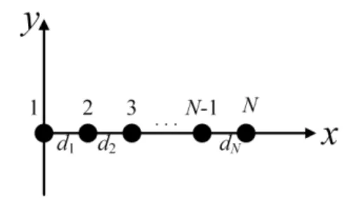
NALYSISOFARRAYFACTORThe linear antenna array parameters generally involve inter-element spacing, excitation amplitude, and number of elements, which directly influences its effect on array factor (AF). All these variables have been used to demonstrate beam forming and beam steering of a linear array. Fig. 1 shows a linear antenna array in which identical antenna elements are placed on one side from the origin.
Brazilian Microwave and Optoelectronics Society-SBMO received 23 Feb 2017; for review 02 Mar 2017; accepted 14 May 2017
N
i
kd i
i i e a AF
1
) cos (
(1)
where N is the number of antenna elements, ai, di, ϕi, and k are the excitation amplitude, the inter-element spacing, the excitation phase and the propagation constant for the ith element. To study the effects of these variables for an optimum design, a MATLAB routine has been developed using Eq. (1), and the AF has been plotted as a function of various control parameters.
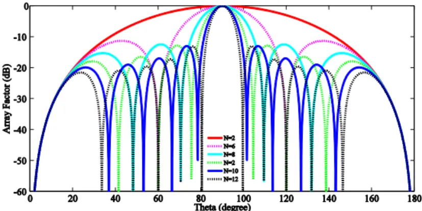
Fig. 2. AF varied for element N from 2 to 12
Because the element N in an antenna array plays an important role in beam forming, beam steering, and interference reduction. Fig. 2 is plotted by varying the number of elements while keeping the spacing between two consecutive elements
as 0.5λ and ϕi = 90°. Results of Fig. 2 are normalized with respect to the
maximum value of the main lobe. From the Fig. 2, it has found that the HPBW is decreased with a minor reduction in the SLL with an increase in the number of elements.
Fig. 3. AF varied with distance, d decreasing from λ/2 to λ/10.
Brazilian Microwave and Optoelectronics Society-SBMO received 23 Feb 2017; for review 02 Mar 2017; accepted 14 May 2017
separation between two array elements, i.e., up to d = λ/10 shown in Fig. 3. It has demonstrated that the distance d should be closer to λ/2.
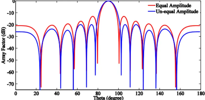
Fig. 4. AF varied for equal and unequal excitation amplitude.
Excitation amplitude for each individual element, commonly known as a weight factor, also changes radiation characteristics of an array antenna. By changing its value for various elements of an array, one can change the overall array pattern. A comparative analysis of weighted and un-weighted antenna design is presented in Fig. 4. This is a primitive analysis, which is not based on the appropriately weighted amplitudes rather than the amplitudes are changed to observe its effect on AF variation. For equal and unequal amplitude excitation, the HPBW is decreased and the SLL is increased while for unequal amplitude excitation, the SLL is reduced and the HPBW is increased shown in Fig. 4.
III. PARTICLE SWARM OPTIMIZATION ALGORITHM
The PSO is frequently used to solve successfully complex multidimensional optimization problems in different fields, such as antenna design and device- modeling [14]-[25] etc. In the PSO, every individual entity in the swarm is referred to as a particle and is associated with a velocity. All particles move in search of space and update their velocity according to the best position which is already found by themselves and by their neighbor which is also trying to find the best position. The PSO is a computational method which iteratively optimizes the problem based on a certain fitness function. Since we are dealing with both uniform and non-uniform linear antenna array, so each particle is a vector which contains the information for each feed antenna. This information includes the excitation amplitude
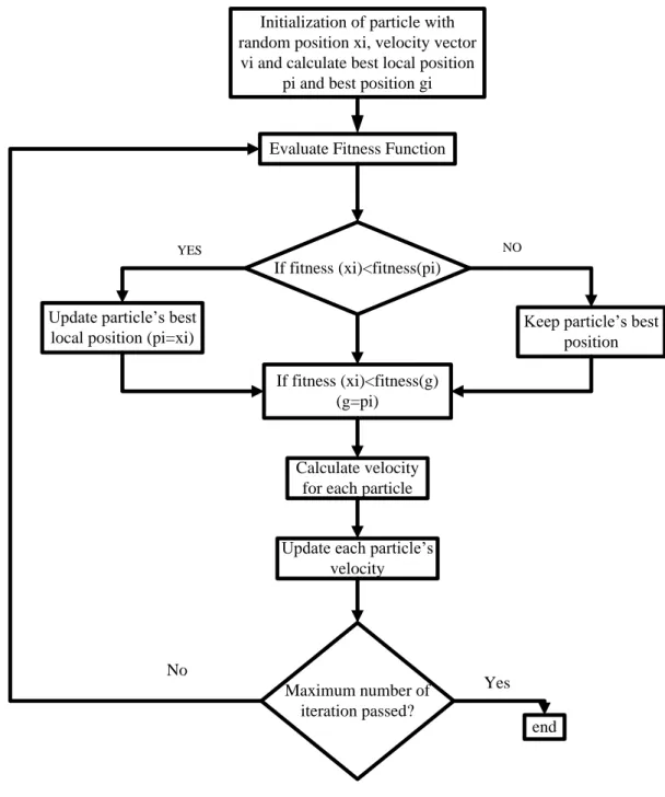
|ai|, excitation phase | ϕi| and the distance of element with respect to the previous position, d in the array. The flow chart of t h e PSO is given in Fig. 5 and t h e PSO algorithm can be summarized as:
For each particle i = 1... S.
i. Generate random di , ai and ϕi where xi=[di |ai| ϕi] and range for |a|, |ϕ| and d is [0,1], [0,3600], [dmax, dmin], respectively.
ii. Initialize individual particle velocities:
)
,
(
max min max min, U d d d d
vid
) ,
( max min max min
, U a a a a
Brazilian Microwave and Optoelectronics Society-SBMO received 23 Feb 2017; for review 02 Mar 2017; accepted 14 May 2017
)
,
(
max min max min,
U
viiii. Compute fitness function for each particle.
Compute the particle’s best position (pi) and the global best position (g) such that f (pi ) < f (g)
Initialization of particle with random position xi, velocity vector
vi and calculate best local position pi and best position gi
Update particle’s best
local position (pi=xi) Keep particle’s best position
If fitness (xi)<fitness(g) (g=pi)
Calculate velocity for each particle
Update each particle’s
velocity
If fitness (xi)<fitness(pi)
Maximum number of iteration passed?
end Evaluate Fitness Function
Yes No
YES NO
Fig. 5. Flow chart of PSO After the initialization phase, the optimization steps are as follows:
i. For each particle i = 1, …, S do:
Brazilian Microwave and Optoelectronics Society-SBMO received 23 Feb 2017; for review 02 Mar 2017; accepted 14 May 2017 ) ( ) ( , , , .
,d id p p id id g g d id
i v r p x r g x
v
)
(
)
(
, , ,,
,a i a p p i a i a g g a i a
i v r p x r g x
v
) (
)
( , , ,
,
, a i a p p i a i a g g a i a
i v r p x r g x
v
where β= 1, αp = 0.9, αg = 0.9
After updating velocity this algorithm will repeat till certain termination criteria like a total number of iteration are met. The PSO requires appropriate fitness function for the algorithm. A fitness function should have the ability to reduce the SLL and minimize the HPBW. A fitness function is designed considering the target value of the SLL and the HPBW. It is given in (2) and (3).
IV. SYNTHESISOFLINEARANTENNAARRAYUSINGPSO
In this section, the PSO is employed for optimum values of excitation amplitude and inter-element spacing to minimize the SLL and HPBW. In order to compare with previous research work, three elements 10, 12, 16 are considered as examples to simulate.
else B SLL A HPBW B HPBW A SLL if SLL HPBW f ) ) (max( ) ) min( ) min( & ) min( ) min( ) min( 0 0 0 0
1 (2)
)) (
max( 1
2 AF d
f (3)
where AF1 AF 2, A0 and B0 are the fixed values of the HPBW and the SLL that keep the
SLL and the HPBW less than A0 and B0, and θd is the angle at which null can be controlled. In the first section fitness function ‘f1’ is employed to minimize the SLL so as to get the optimum values of excitation amplitude and inter-element spacing. While in the second section ‘f2 ‘ is used to control the nulls in a specified direction.
A. Optimization of Excitation Amplitude
Brazilian Microwave and Optoelectronics Society-SBMO received 23 Feb 2017; for review 02 Mar 2017; accepted 14 May 2017
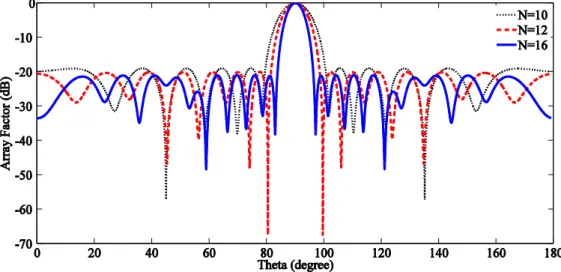
Fig. 6. AF varied with optimized excitation amplitude
TABLE.I. COMPARATIVE RESULTS FOR OPTIMIZED EXCITATION AMPLITUDE.
` Proposed PSO BBO [26] CFO [27] GA [28]
No. elements 10 12 16 10 10 16
Max SLL (dB) -17.26 -24.14 -28.05 -15.97 -15.93 -16.07
HPBW(degree) 11 9 7 — — —
TABLE. II. OPTIMIZED VALUES FOR EXCITATION AMPLITUDE WITH FIXED SPACING AND PHASE
amplitude N=16 N=12 N=10 a1 0.2127 0.3087 0.3881 a2 0.2287 0.3938 0.4097 a3 0.3606 0.4444 0.6289 a4 0.3606 0.5530 0.6322 a5 0.5198 0.7159 0.6778 a6 0.5627 0.7115 0.6008 a7 0.6373 0.7725 0.6012 a8 0.6496 0.6733 0.4768 a9 0.7127 0.6166 0.5620 a10 0.7088 0.5146 0.2291 a11 0.5694 0.3158 a12 0.5113 0.3113 a13 0.4545
Brazilian Microwave and Optoelectronics Society-SBMO received 23 Feb 2017; for review 02 Mar 2017; accepted 14 May 2017
The excitation amplitude is assumed as the range [0 1]. For uniform inter-element spacing and excitation phase, the proposed PSO algorithm has a peak value of -17.26 dB with the minimum HPBW as 11° when 10 antenna elements are selected. For N = 12 case, the peak SLL is less than -24.14 dB while the HPBW decreases to 9°. Similarly, for N = 16 case the peak SLL is further reduced to -28.05 dB and the HPBW is less than 7° shown in Fig. 6. It has been found that there is an improvement of 1.29 dB and 11.98 dB in the SLL compared with the results of the BBO [26] and the GA [28] for N = 10 and N = 16, respectively. Considerable improvement in the HPBW has been observed while the SLL is suppressed with increasing number of elements listed in Table I.
B. Optimization of Inter-element spacing
The performance of an antenna array is also dependent on the distance between two consecutive elements. To obtain the optimum values of inter-element spacing, the PSO algorithm has been employed with equal excitation amplitude ai = 1 and excitation phase ϕi = 90° by using the fitness function f associated with the SLL and HPBW. The number of elements in the antenna array has been chosen as 10, 12, and 16.
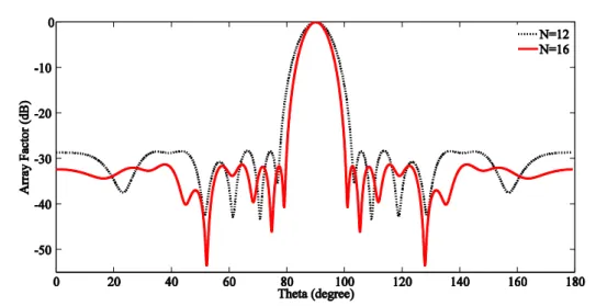
Fig. 7. Plot of AF when inter-element spacing was optimized
TABLE .III. COMPARATIVE RESULTS FOR OPTIMIZED I N T E R -ELEMENT SPACING.
Proposed PSO BBO [26] PSO [29]
No. of elements 10 12 16 10 10
Max SLL (dB) -19.10 -20.09 -21.08 -18.14 -17.82
HPBW(degree) 11 7 5 — 8.9
Brazilian Microwave and Optoelectronics Society-SBMO received 23 Feb 2017; for review 02 Mar 2017; accepted 14 May 2017
TABLE. IV. OPTIMIZED VALUES FOR SPACING WITH FIXED EXCITATION AMPLITUDE AND PHASE. Spacing N=16 N=12 N=10
d1 0.7851 0.7141 0.7022 d2 0.8143 0.7070 0.5621 d3 0.6368 0.5496 0.4684 d4 0.5386 0.5183 0.4233 d5 0.5820 0.4100 0.4780 d6 0.4491 0.4719 0.4932 d7 0.5882 0.4884 0.6535 d8 0.4074 0.5118 0.6926 d9 0.4277 0.6436 0.4929 dd0 0.4955 0.8274 d11 0.5096 0.5958 d12 0.4741 d13 0.7078 d14 0.7736 d15 0.8566
C. Optimiza tion of Excita tion Amplitude and Inter -element spa cing
The PSO method is also employed to optimize the excitation amplitude and inter-element spacing. The fitness function given by Eq. (2) is used to get the optimum amplitude and position so as to minimize the SLL and the HPBW. In Table V, the observations are made for N = 12, 16 and the results are compared with previous research work [1].
TABLE. V. COMPARATIVE RESULTS FOR MINIMUM SLL AND HPBW WHEN N = 12, 16
Proposed PSO RGA[1]
No. of elements 12 16 12 16
Max SLL (dB) -28.29 -31.29 -13.56 -15.18
HPBW(degree) 9 7 9.55 8.45
Brazilian Microwave and Optoelectronics Society-SBMO received 23 Feb 2017; for review 02 Mar 2017; accepted 14 May 2017
Fig. 8. AF varied with optimized inter-element spacing and excitation amplitude
V. DIRECTIVITYANDNULLCONTROL
The directivity of the antenna can be defined as the ratio of radiation intensity in a given direction from the antenna /antenna array to the radiation intensity averaged over all directions [13]. The mathematical form of directivity, D for antenna arrays can be written as
r a d P
U
D
4
max (4)2 max
) max( AF
AF
U (5)
d d U
Pr a d
20 0
) sin( )
( (6)
where Prad is the total radiated power and Umax is the maximum radiation intensity.
N=12 N=16
Fig. 9. 2D plot of directivity for optimized excitation amplitude and inter-element spacing 0o<ϕ <360o
Brazilian Microwave and Optoelectronics Society-SBMO received 23 Feb 2017; for review 02 Mar 2017; accepted 14 May 2017
The directivity of the linear antenna array can be improved by controlling the switching time [30], inter-element spacing and excitation amplitude. Considering 12 and 16 antenna array elements, the directivity and the SLL of linear antenna arrays have been improved by increasing the number of elements and controlling the inter-element spacing, the excitation amplitude. table VI. is listed the comparative results for the directivity and the SLL.
TABLE VI. COMPARATIVE RESULTS FOR DIRECTIVITY AND SLL
No. of elements Algorithms Directivity (dB) SLL (dB) 12 Proposed 10.4100 -28.29 16 Proposed 11.3764 -31.29 16 DE[30] 11.4683 -18.74 16 PSO[30] 11.4515 -18.73 16 RGA[30] 11.4027 -17.8
Another important application of linear array is null control [1], [5]-[6], [9]. The null control refers to control the radiation pattern in a way such that a relatively small amount of power is received/radiated in certain directions. At the transmitting end, the null control is used for transmitting low power in the directions where an eavesdropper is present. On the receiving side, it is used to reduce the amount of power received from interferers. The null control can be achieved by controlling the parameters, excitation amplitude, excitation phase, array spacing and the number of elements. It is important to note that reducing the amount of power in one direction means that power is increased in another direction. Ideally, the power is decreased in the direction of interferers and the main beam is increased in the same direction. Generally, it is hard to accomplish this, it is needed to tradeoff. So the PSO algorithm is employed to place nulls in specified directions using the fitness function f2. Three different examples are considered for different antenna elements and nulls at specified places.
TABLE VII. SLL, HPBW AND NULL DEPTH WHEN NULLS ARE IMPOSED AT θd=500, 550, 1250 AND 1300
N HPBW (degree) SLL (dB) Null depth at 500 Null depth at 550
10 11 -10 -55.9 dB -55.5 dB
12 9 -11 - 48.1 dB -49.1 dB
16 7 -11.6 - 57 dB -57 dB
In order to validate the PSO algorithm, a linear antenna array of N = 10, 12 and 16 elements is analyzed, respectively, with the nulls imposed at θ=500, 550, 1250 and 1300. The PSO is employed with the appropriate fitness function to control the nulls at specified angular direction. Table VII is listed the values of the SLL, the HPBW and the null depth for imposed nulls at θ =500
Brazilian Microwave and Optoelectronics Society-SBMO received 23 Feb 2017; for review 02 Mar 2017; accepted 14 May 2017
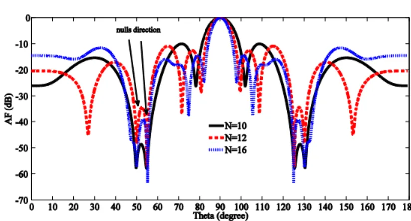
Fig. 10. Plot of AF when nulls are imposed at θ=500, 550, 1250 and 1300.
TABLE VIII. OPTIMIZED VALUES OF EXCITATION AMPLITUDE WHEN NULLS ARE PLACED AT θd=500, 550, 1250 AND
1300
.
No. of elements 10 12 16
Excitation Amplitude
0.2658 0.3465 0.3931 0.3578 0.7744 0.2958 0.8053 0.5334 0.5136 0.4794 0.5146 0.5263 0.4630 0.2835 0.4735 0.2575 0.6050 0.7563 0.3758 0.7625 0.1670 0.6736 0.3483 0.5305 0.4199 0.3025 0.7270 0.3397 0.5249 0.5964 0.5333 0.9566 0.5828 0.0093 0.8880 0.4377 0.7248 0.1519 Fig. 10 is plotted the AF is varied for imposed nulls at θ =500
, 550, 1250 and 1300. Table VIII is given the optimized value of inter-element spacing for the nulls located at θ =500
, 550, 1250 and 1300.
Brazilian Microwave and Optoelectronics Society-SBMO received 23 Feb 2017; for review 02 Mar 2017; accepted 14 May 2017
TABLE IX. OPTIMIZED VALUES OF EXCITATION AMPLITUDES WHEN NULLS ARE IMPOSED AT θ=700, 800, 1000 AND
1100
No. of elements 10 12 16
Excitation amplitudes (ai)
0.6728 0.2699 0.5232 0.4838 0.4973 0.0718 0.2651 0.6247 0.3344 0.6880 0.6089 0.4895 0.2896 0.8114 0.6623 0.6536 0.2136 0.1877 0.5125 0.7713 0.8941 0.3148 0.8532 0.6679 0.4445 0.2267 0.5754 0.8132 0.8313 0.5494 0.3379 0.6393 0.8596 0.5239 0.3096 0.2282 0.2692 0.2932
Fig. 11. The plot of AF when nulls are imposed at 700, 800, 1000 and at 1100. TABLE X SLL, HPBW AND NULL DEPTH WHEN NULLS ARE IMPOSED AT θ=700, 800, 1000 AND 1100.
N HPBW (degree) SLL (dB) Null depth at 700 Null depth at 800
10 9 -10.4 -59.00 dB -32.1 dB
12 9 -12 -51.55 dB -51.1 dB
16 7 -16 -52 dB -53.3 dB
Brazilian Microwave and Optoelectronics Society-SBMO received 23 Feb 2017; for review 02 Mar 2017; accepted 14 May 2017 VI. CONCLUSION
In this paper, it has developed the PSO algorithm code to calculate and optimize the inter-element spacing and excitation amplitude, which the optimization objectives targeted in this work are involved the HPBW, the SLL, directivity and null steering in certain angular directions. In order to achieve these goals, the two fitness functions have been used in the PSO method. One of the fitness functions is used with different values for the number of antenna array elements to find the optimum values of excitation amplitude and inter-element spacing that give a pattern having minimum SLL and HPBW. PSO employs the second fitness function to control the nulls in a specified direction and minimize SLL and HPBW by optimizing excitation amplitude.
REFERENCES
[1] B. Goswami and D. Mandal, “Nulls and Sidelobe Levels Control in a Time Modulated Linear Antenna Array by Optimizing Excitations and Element Locations Using RGA,” Journal of Microwaves, Optoelectronics, and Electromagnetic Applications, Vol. 12, No. 2, December 2013.
[2] T. Girard, R. Staraj, E. Cambiaggio and F. Muller, “A simulated annealing algorithm for planar or conformal antenna array synthesis with optimized polarization,” Microwave and Optical Technology Letters, Vol. 28, No. 2, pp. 86-89, 2001.
[3] C. M. Coleman, E. J. Rothwell and J. E. Ross, “Investigation of simulated annealing, ant-colony optimization, and genetic algorithms for self-structuring antennas,” IEEE Transactions on Antennas and Propagation, Vol. 52, No. 4, pp. 1007-1014, 2004.
[4] D. Marcano and F. Duran, “Synthesis of antenna arrays using genetic algorithms,” IEEE Antennas and Propagation Magazine, Vol. 42, No. 3, pp. 12-20, 2000.
[5] D. I. Abu-Al-Nadi, T. H. Ismail and M. J. Mismar, “Synthesis of linear array and null steering with minimized side-lobe level using particle swarm optimization,” Proceedings of the 4th European Conference on Antennas and Propagation, pp. 1-4, 2010.
[6] M. M. Khodier and C. G. Christodoulou, “Linear array geometry synthesis with minimum sidelobe level and null control using particle swarm optimization,” IEEE Transactions on Antennas and Propagation, Vol. 53, No. 8, pp. 2674-2679, 2005.
[7] J. Song, H. Zheng and L. Zhang, “Application of particle swarm optimization algorithm and genetic algorithms in beam broadening of phase array antenna,” International Symposium on Signals, Systems and Electronics (ISSSE), pp. 17-20, 2010.
[8] M. Y. X. Lia, “Optimal synthesis of linear antenna array with composite differential evolutionary algorithm,” Scientia Iranica, Vol. 19, No. 9, pp. 1780-1787, 2012.
[9] B. Goswami and D. Mandal, “A genetic algorithm for the level control of nulls and side lobes in linear antenna arrays,” Journal of Computer and Information Sciences, Vol. 25, No. 2, pp. 117-126, 2013. [10] S. K. Gotsis, K. Siakavara, E. Vafiadis and J. Sahalos, “A multi-objective approach to subarrayed linear
antenna arrays design based on memetic differential evolution,” IEEE Transactions on Antennas and Propagation, Vol. 61, pp. 3042-3052, 2013.
Brazilian Microwave and Optoelectronics Society-SBMO received 23 Feb 2017; for review 02 Mar 2017; accepted 14 May 2017
[13] C. A. Balanis, “Antenna Theory Analysis and Design”, A John Wiley and sons, 2005.
[14] G. Ram, D. Mandal, R. Kar and S. P. Ghosal, “Synthesis of time modulated linear antenna arrays using particle swarm optimization,” IEEE Region 10 Conference TENCON, pp. 1-4, 2014.
[15] A. Banookh, and S. M. Barakati, “Optimal Design of Double Folded Stub Microstrip Filter by Neural Network Modelling and Particle Swarm Optimization,” Journal of Microwaves, Optoelectronics and Electromagnetic Applications, Vol. 11, No. 1, June 2012.
[16] F. R. Durand, and T. Abrão, “Particle Swarm Optimization in WDM/OCDM Networks with Physical Impairments,” Journal of Microwaves, Optoelectronics and Electromagnetic Applications, Vol. 12, No. 2, December 2013.
[17] C. J. A. Bastos-Filho and E. M. N. Figueiredo, “Design of Distributed Optical-Fiber Raman Amplifiers using Multi-objective Particle Swarm Optimization” Journal of Microwaves, Optoelectronics and Electromagnetic Applications, Vol. 10, No. 2, December 2011.
[18] A. Banookh, and S. M. Barakati, “Optimal Design of Double Folded Stub Microstrip Filter by Neural Network Modelling and Particle Swarm Optimization” Journal of Microwaves, Optoelectronics and Electromagnetic Applications, Vol. 11, No. 1, June 2012.
[19] L. Wakrim, S. Ibnyaich, and M. M. Hassani, “The study of the ground plane effect on a Multiband PIFA Antenna by using Genetic Algorithm and Particle Swarm Optimization” Journal of Microwaves, Optoelectronics and Electromagnetic Applications, Vol. 15, No. 4, December 2016.
[20] S. S, Travessa, and W. P. Carpes Jr., “Use of an Artificial Neural Network-based Metamodel to Reduce the Computational Cost in a Ray-tracing Prediction Model” Journal of Microwaves, Optoelectronics and Electromagnetic Applications, Vol. 15, No. 4, December 2016.
[21] P. J. Bevelacqua and C. A. Balanis, “Minimum side lobe level for linear array,” IEEE Transactions on Antennas and Propagation, Vol. 55, No. 12, pp. 3442 - 3449, 2007.
[22] A. R. Harish and M. Sachidananda, Antennas and Wave Propagation, Oxford University Press, 2007. [23] K. Kennedy and R. Eberhart, “Particle swarm optimization,” Proceedings of the IEEE International
Conference on Neural Networks, pp. 1942-1948, 1995.
[24] M. A. Haq, M. T. Afzal, U. Rafique, Q. D. Memon, M. A. Khan and M. M. Ahmed, “Log periodic dipole antenna design using particle swarm optimization,” International Journal on Electromagnetics and Applications, Vol. 2, No. 4, pp. 65-68, 2012.
[25] Q. D. Memon, M. M. Ahmed, N. M. Memon and U. Rafique, “An efficient mechanism to simulate DC characteristics of GaAs MESFETs using swarm optimization,” 9th IEEE International Conference on Emerging Technologies (ICET), pp. 1-5, 2013.
[26] A.Sharaqa and N. Dib, “Design of linear and elliptical antenna arrays using Biogeography Based Optimization,” Arab Journal of Science and Engineering, Vol. No. 4,pp 2929–2939, 2013.
[27] G.Al-Kubati, “Central force optimization method and its application to the design of antennas,” Master Thesis, Jordan University os science and Technology, 2009.
[28] P. Joshi, and N. Jain, “Optimization of linear antenna array using genetic algorithm for a reduction in side lobe levels and to improve directivity,” International Journal of Latest Trends in Engineering and Technology (IJLTET), Vol. 2, No. 3, 2013. Vol. 28, pp 540–549, 2014.
[29] L. Pappula, and D. Ghosh, “Linear antennaarray synthesis using Cat Swarm Optimization,” International Journal of Electronics and Communication (AEU), Vol. 28, No. 6, pp 540–549, 2014.