EXTERIOR ORIENTATION ESTIMATION OF OBLIQUE AERIAL IMAGERY USING
VANISHING POINTS
Styliani Verykokou*, Charalabos Ioannidis
Laboratory of Photogrammetry, School of Rural and Surveying Engineering, National Technical University of Athens, Greece [email protected], [email protected]
Commission III, WG III/1
KEY WORDS: Oblique Aerial Images, Vanishing Point, Nadir Point, True Horizon Line, Exterior Orientation, Georeferencing
ABSTRACT:
In this paper, a methodology for the calculation of rough exterior orientation (EO) parameters of multiple large-scale overlapping oblique aerial images, in the case that GPS/INS information is not available (e.g., for old datasets), is presented. It consists of five main steps; (a) the determination of the overlapping image pairs and the single image in which four ground control points have to be measured; (b) the computation of the transformation parameters from every image to the coordinate reference system; (c) the rough estimation of the camera interior orientation parameters; (d) the estimation of the true horizon line and the nadir point of each image; (e) the calculation of the rough EO parameters of each image. A developed software suite implementing the proposed methodology is tested using a set of UAV multi-perspective oblique aerial images. Several tests are performed for the assessment of the errors and show that the estimated EO parameters can be used either as initial approximations for a bundle adjustment procedure or as rough georeferencing information for several applications, like 3D modelling, even by non-photogrammetrists, because of the minimal user intervention needed. Finally, comparisons with a commercial software are made, in terms of automation and correctness of the computed EO parameters.
* Corresponding author
1. INTRODUCTION
For many decades the photogrammetric procedures were adjusted almost exclusively in vertical aerial imagery, thus preventing datasets of oblique airborne images from being exploited for the acquisition of metric information. This kind of imagery was used mainly for reconnaissance or interpretation purposes and visual inspection of the physical or built environment. In recent years, multi-camera systems have become a well-established technology for several applications and oblique aerial images are used more and more for several metric applications, including 3D modelling, cadastre, mapping, tax assessment and geometric documentation of constructions. Furthermore, Unmanned Aerial Vehicles (UAVs) are capable of capturing oblique images, which may be used not only as a complementary dataset for a mapping project consisting of traditional vertical airborne or terrestrial imagery, but also as the basic source of information for various kinds of applications. The main prerequisite for the processing of oblique imagery datasets is the availability of rough orientation information, which is usually obtained via a GPS/INS system and/or ground control points (GCPs) well distributed all over the block of aerial images.
Over the last decade, much research has been conducted on the georeference of datasets which include oblique aerial images. Smith et al. (2008) oriented a block of oblique aerial images, using initial georeferencing information and numerous GCPs as inputs, through commercial software. Gerke and Nyaruhuma (2009) introduced the incorporation of geometric scene constraints into the triangulation of oblique aerial imagery, using approximations for the exterior orientation (EO)
parameters and GCPs. Fritsch et al. (2012) georeferenced datasets of oblique aerial imagery using orientation information from a GPS/IMU system. Wiedemann and Moré (2012) discussed some orientation strategies for oblique airborne images acquired with a calibrated multi-camera system mechanically connected with a DGPS/IMU system. Rupnik et al. (2013) presented an approach which relied on open-source software for the orientation of large datasets of oblique airborne images provided with georeferencing information, thus eliminating the need for ground control. Karel et al. (2013) developed a software which, inter alia, georeferences oblique aerial images in two steps that include the co-registration of the images and the georeferencing of the resulted block as a whole, using image meta-information (footprints, flying height, interior orientation) as well as pre-existing orthophoto maps and DSMs/DTMs for the extraction of control points and the computation of their heights. Geniviva et al. (2014) combined image registration techniques with GPS/IMU information and existing orthorectified imagery to automatically georeference oblique images from high-resolution low-altitude, low-cost aerial systems, while Zhao et al. (2014) implemented direct georeferencing approaches for oblique imagery in different coordinate systems using GPS/INS data.
All the above mentioned approaches on georeferencing oblique aerial image datasets require initial approximations for the EO parameters. Furthermore, for many other applications, such as 3D modelling using oblique and vertical airborne imagery (Smith et al., 2009) or automatic registration of oblique aerial imagery with map vector data (Habbecke and Kobbelt, 2012), initial orientation information is required. Other applications rely on the availability of a rough estimation of the EO, which
is refined via matching image features among multi-view oblique aerial images for their registration (Saeedi and Mao, 2014) or via matching oblique image features with features extracted from an untextured 3D model of the scene for texture mapping (Frueh et al., 2004; Ding et al., 2008; Wang and Neumann, 2009).
In this paper a methodology for the automatic determination of approximate EO parameters of multiple overlapping oblique aerial images, in the case that information by on-board sensors for positioning and attitude determination is not available, is proposed (e.g., for old datasets of oblique images, UAV images without GPS/INS metadata). It relies on image matching for transferring the geospatial information among images and implements automatic detection of the nadir point of every image using edge and line extraction algorithms, combined with robust model fitting and least-squares techniques. The user intervention required is limited to the measurement of a minimum number of points in only one image of the block and the input of their ground coordinates, which may be extracted from a free Earth observation system, like Google Earth, as well as to the input of the average flying height and ground elevation.
2. METHODOLOGY
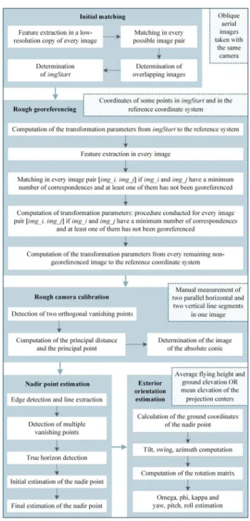
In this section, the proposed methodology for the rough estimation of the EO parameters of multiple overlapping oblique aerial imagery is presented. It consists of five main steps and is illustrated in Figure 1.
2.1 Initial Matching between Images
The first step of the proposed methodology is the automatic determination of the overlapping images and the automatic definition of the starting image, in which the GCPs have to be measured. The images are resampled to a sufficiently low resolution and feature points are detected in every image using the SIFT algorithm (Lowe, 2004). The choice of this algorithm is made on the grounds that SIFT feature points are scale and rotation invariant and provide a robust matching across a substantial range of affine distortion, changes in 3D viewpoint, illumination changes and addition of noise. Several tests performed for this study using multi-view oblique aerial images showed that the matching of SIFT features leads to better results than the computationally less expensive matching of SURF features (Bay et al., 2006).
At the stage of image matching, the extracted feature points of an image are compared to the extracted feature points of all the other images, using the criterion of the minimum Euclidean distance between their descriptors and the ratio test, proposed by Lowe (2004). Furthermore, the correspondences are geometrically verified via the RANSAC algorithm (Fischler and Bolles, 1981), through the computation of the fundamental matrix, using the eight-point algorithm (Hartley, 1997). The detected correspondences may still contain some outliers which, however, are of minor importance for the results of this step. The first output of this procedure is the number of matches between every pair of images, which determines whether they are overlapping, so that the search of correspondences during the subsequent step of rough georeferencing takes place only in overlapping images for the minimization of the processing time. The second output is the image in which the points of known coordinates have to be measured, which is defined as the image with the maximum number of overlapping images.
Figure 1. The proposed methodology
2.2 Rough Georeferencing
The georeferencing of the images is based on the measurement of a minimum number of GCPs in only one image and the transferring of the geospatial information among images.
2.2.1 Selection of the Appropriate Transformation: The required number of GCPs depends on the transformation that is used to express the relation between the starting image and the coordinate reference system (CRS). Specifically, three points are required in the case of the six-parameter affine transformation and four points in the case of the eight-parameter projective transformation (homography). Except for these transformations, the polynomial transformations of second, third, fourth and fifth order were tested in low and high oblique aerial imagery and the results proved that the affine as well as the projective transformation were far more suitable. This is explained by the fact that if a second or higher degree
polynomial transformation expresses the relation between two images as well as between the starting image and the CRS, the transformation of every other image to the CRS is expressed by a polynomial of higher order, depending on the number of transformations involved between the image and the CRS. However, high order polynomials produce significant distortions. In contrast, the combination of affine or projective transformations does not change the type of the resulting transformation. The homography yields better results than the affine transformation in cases of low altitude high oblique aerial images, because of their trapezoidal footprint that cannot be approximated by a rectangle.
2.2.2 Calculation of the Transformation Parameters: The first step of the georeferencing procedure is the computation of the transformation parameters from the starting image to the CRS. Then, a matching procedure is applied only in the overlapping images, if at least one of them has not been georeferenced, using the SIFT algorithm. The similarity of the descriptors is determined based on the minimum Euclidean distance, the ratio test is implemented and the RANSAC algorithm is applied for the rejection of incorrect matches via the estimation of the fundamental matrix. However, a point to point constraint needs to be imposed because some outliers still remain. For this reason, the affine or the projective transformation, depending on the scene depicted in the images, is fitted to the correspondences via RANSAC, using a distance threshold for the determination of the outliers, which depends on the dimensions of the images. The transformation parameters between the images of each pair are computed via least-squares adjustment using their initial estimation obtained by RANSAC and the inliers returned by the same algorithm. If one of the images being matched is georeferenced and if the number of valid correspondences is greater than a threshold, the transformation parameters from the non-georeferenced image to the CRS are calculated. This threshold is defined in order to crosscheck that georeferencing information is transferred among overlapping images. If none of the images are georeferenced, only their transformation parameters are stored. Some images may pass through this step without having been georeferenced because either their overlapping images are not georeferenced or the number of detected correspondences is not big enough. The transformation parameters from each remaining non-georeferenced image to the CRS are computed using the estimated transformation parameters between this image and its corresponding georeferenced one with the maximum number of matches. The main output of the georeferencing procedure is the parameters that define the transformation between each image and the CRS.
2.3 Rough Camera Calibration
The principal distance and the location of the principal point are fundamental prerequisites for the computation of an initial estimation of the nadir point of each image, using the detected true horizon line, and the estimation of the angular orientation of the camera for each image in terms of tilt, swing and azimuth. If the camera interior orientation is unknown, these parameters are roughly computed. The principal point is considered to coincide with the image center. The principal distance may be determined using the estimation of the principal point if two vanishing points and the angle between the two sets of parallel 3D lines that converge to these vanishing points are known (Förstner, 2004). According to the proposed methodology, the principal distance is calculated using the vanishing points of two perpendicular directions,
which may be easily indicated manually without particular knowledge of the scene geometry. This is achieved by measuring two parallel horizontal line segments and two vertical ones. The intersection point of each set of parallel segments is the vanishing point of the corresponding direction. The camera constant (c) is calculated according to equation (1).
H P N P H P N P
c x x x x y y y y (1)
where xP, yP = image coordinates of the principal point
xN, yN = image coordinates of the nadir point
xH, yH = image coordinates of the vanishing point of a
horizontal direction
It has to be mentioned that in the case of images taken with a camera with a low quality lens system, the lens distortion effect has to be corrected before the next steps, because straight lines in space would be mapped to curves in the images, thus leading to an incorrect estimation of the nadir point. In this case, the principal point, the principal distance and the lens distortion coefficients have to be known. Once the camera is calibrated, the image of the absolute conic can be computed. The absolute conic is a second degree curve lying on the plane at infinity, consisting of complex points (Hartley and Zisserman, 2003). The image of this curve is an imaginary point conic that depends on the camera interior orientation, being independent on the camera position or orientation. Thus, for all the images taken by the same camera, the image of the absolute conic, ω, is the same. It is represented by a 3x3 matrix and is calculated via equation (2), using the calibration matrix K and considering zero skew and unit aspect ratio, to wit, square pixels.
T
1 0; 0
0 0 1
P
P
c x
c y
ω ΚΚ K (2)
2.4 Nadir Point Detection
A basic step of the proposed methodology is the detection of the nadir point of every image, which is the vanishing point of the vertical dimension and lies in the intersection between the vertical line from the perspective center with the image plane.
2.4.1 Extraction of Line Segments: The initial step is the extraction of edges using the Canny operator (Canny, 1986). The “high” threshold, which is used in its hysteresis thresholding step, is automatically calculated according to the Otsu algorithm (Otsu, 1979) as proposed by Fang et al. (2009), while the “low” threshold is set to be the half of the “high” one. Subsequently, the Progressive Probabilistic Hough Transform (Matas et al., 1998) is applied in the binary edge map for the extraction of line segments.
2.4.2 Detection of Multiple Vanishing Points: The detection of multiple vanishing points is the next step. A variation of the RANSAC algorithm is applied for the estimation of the intersection point of most line segments. According to this variation, the random iterative choice of two line segments is controlled so that the initial estimation of their intersection point lies outside the image limits, having a smaller y coordinate than the height of the image (assuming that the origin of the image coordinate system is located at the top left corner, x-axis points to the right and y-axis points downwards). This constraint is imposed in order to ensure that mostly
vanishing points of horizontal directions will be detected, taking into consideration the fact that the nadir point is located below the bottom limit of an oblique aerial image and assuming that the true horizon line lies outside the image, towards its upper side. Subsequently, the estimation of the detected vanishing point is refined through least-squares adjustment, using its initial estimation and the inliers that converge to this point obtained by RANSAC. Then, the horizontal line segments that converge to the detected vanishing point are removed from the set of line segments. This procedure is repeated for the detection of a sufficient number of vanishing points.
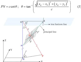
2.4.3 Detection of the True Horizon Line: The true horizon line is the intersection between the horizontal plane that contains the projection center and the oblique image plane. All the horizontal line segments converge to this line, which consists of the vanishing points of horizontal directions. The true horizon line is estimated via a variation of the RANSAC algorithm as the line that connects most detected vanishing points. The iterative random choice of two vanishing points is controlled in order to ensure that the initial estimation of the nadir point, which is obtained based on the estimation of the equation of the true horizon line using the two random vanishing points, has a greater y coordinate than the image
height. The estimation of the nadir point is obtained according to equation (3), where θ is the depression angle, PN is the
distance between the principal point and the nadir point and xK,
yK are the image coordinates of the intersection point K between
the true horizon line and the principal line (Figure 2). The latter one is determined based on the fact that it is perpendicular to the true horizon line and passes through the principal point (Verykokou and Ioannidis, 2015).
2
21
cot ; tan
K P K P
x x y y
PN c θ θ
c (3)
Figure 2. Tilt, swing and azimuth in an oblique aerial image
The nadir point coordinates are determined using the distance
PN and the coordinates of the principal point, knowing that the
nadir point lies on the principal line. In the resulting system of two equations, the solution according to which the nadir point is located below the principal point is the correct one. The estimation of the true horizon line made by RANSAC is refined through least-squares adjustment using the vanishing points that are characterized as inliers by RANSAC. In this way, the final estimation of the true horizon line is obtained.
2.4.4 Estimation of the Nadir Point: The equation of the principal line is determined, the intersection point between the true horizon line and the principal line is computed, the depression angle and the distance between the principal point
and the nadir point are calculated and an estimation of the nadir point coordinates is obtained. However, this is not the final solution, because the errors arising from the calculation of multiple horizontal vanishing points and the estimation of the equation of the true horizon line are involved.
The horizontal line segments that constitute the inliers are removed from the set of line segments. If the distance between the initial estimation of the nadir point and a line that passes through the endpoints of a remaining segment is greater than a predefined threshold, this segment is considered to be non-vertical and is rejected. A variation of the RANSAC algorithm is used for the final estimation of the nadir point, using the non-rejected line segments. According to this variation, the iterative estimation of the nadir point using two line segments is considered to be correct if (a) the y coordinate of the nadir point
is bigger than the image height, (b) the distance between the nadir point and its initial estimation, obtained using the true horizon line, is smaller than a threshold and (c) the angles between the line segments that converge to the nadir point and the line segments that converge to multiple horizontal vanishing points differ from a right angle by an angular threshold. As far as the third constraint is concerned, multiple horizontal vanishing points are calculated lying in predefined distances on the true horizon line. Let vN be the nadir point estimation and
vHi be the vanishing point of a horizontal direction, both in
homogeneous coordinates; the angle φ between the lines that converge to these vanishing points is computed via equation (4), using the image of the absolute conic ω (Hartley and Zisserman, 2003).
T
T T
cosφ i
i i
N
N N H
H
H
v ωv
v ωv v ωv (4)
The final estimation of the nadir point is obtained through least squares adjustment.
2.5 Rough Exterior Orientation Estimation
The image coordinates of the nadir point and the principal point of every image are transformed to the CRS using the computed rough georeferencing parameters, through an affine or homography transformation. The coordinates of the nadir point in the CRS are the horizontal coordinates of the projection center (X0, Y0). As far as the third coordinate (Z0) is concerned,
the same value for all the projection centers is calculated, using the average flying height and ground elevation.
The tilt (t), swing (s) and azimuth (a) angles are illustrated in
Figure 2. The tilt angle is the complement of the depression angle, which is computed according to equation (3). The swing angle is the angle measured clockwise from the positive yc-axis to the principal line, at the side of the nadir point; yc-axis has its origin at the principal point and is directed upwards. The first step for the computation of the swing angle is the determination of the intersection point (xI, yI) between the principal line and
the upper border of the image (x-axis). Then, the swing angle is calculated geometrically, according to equation (5). The azimuth angle is computed via equation (6).
1
2 2
: if
cos : if
P N P
P N
P I P I
x x
y
s π
x x
x x y y
(5)
1
if and
if and
if and
2 if and
tan 0 if and
if and
2 if and
3 2 if and
P N P N
P N P N
P N P N
P N P N
P N
P N P N
P N
P N P N
P N P N
P N P N
a a' x x y y
a =π- a' x x y < y
a =π+ a' x x y y
a = π- a' x x y y
x x
a'
a = x x y y
y y
a =π x x y y
a =π x x y y
a = π x x y y
(6)
Using these angles, the elements, rij, of the 3×3 rotation matrix are computed according to equation (7) (Dewitt, 1996).
11 12 13 21 22 23 31 2 33 3
cos cos sin cos sin ; cos sin sin cos cos ;
sin sin ;
sin cos cos cos sin ; sin sin cos cos cos ; cos sin ; r sin sin ; sin cos ; r cos
r s a s t a
r s a s t a
r s t
r s a s t a
r s a s t a
r s t t a
r t a t
(7)
Then, the orientation of the camera can be computed in terms of omega (ω), phi (φ) and kappa (κ) according to equation (8) (Dewitt, 1996), or in terms of yaw (y), pitch (p) and roll (r),
using equation (9) (LaValle, 2006).
1 32 1 1 21
31
33 11
tan ; sin ; tan
r r
ω φ r κ
r r (8)
32 2
1 21 1 31 1
11 32 332 33
tan ; tan ; tan
r r r
y p r
r r r r (9)
3. DEVELOPED SOFTWARE
A software suite consisting of three desktop applications has been developed using the Microsoft .NET Framework 4. The first application (Figure 3, top left) aims at the determination of the overlapping images and the starting image, the second one (Figure 3, bottom left) calculates the transformation parameters from every image to the CRS and the third one (Figure 3, right) computes the rough EO parameters of the imagery. The applications are intended for computers running Microsoft Windows; they have been developed in the C# programming language and make use of some functionalities offered by the OpenCV library, using its .Net wrapper, Emgu CV.
The first application, which requires as input only the images, exports an ASCII file that contains the number of correspondences between each possible image pair as well as a file with the name of the starting image. The inputs of the second application are: (a) the images, (b) the ASCII file containing the ground coordinates of some points in the CRS, (c) an ASCII file containing the pixel coordinates of these points in the starting image, which can be replaced by the direct measurement of these points using this application, and (d) the type of transformation (affine or homography). The output of this application is a file containing the transformation parameters from each image to the CRS. In the case of the affine transformation, this file is a world file, which may be used by a GIS in order to rectify the corresponding image. In the case of the homography transformation, the eight parameters are stored in an ASCII file and, using this application, the images are rectified in order to be visualized in
a GIS environment at approximately the correct position, scale and orientation. In this case, the world files store the four parameters of a translation and scaling transformation, while the other two parameters are set to zero. The input data of the third application are: (a) the images, (b) the camera interior orientation, which may be replaced by the measurement of two parallel horizontal and two vertical line segments, (c) the files containing the georeferencing parameters of the images, (d) the type of transformation (affine or homography) and (e) either the average flying height and ground elevation or the average elevation of the projection centers.
Figure 3. Developed software suite
4. RESULTS
The software suite was tested using a dataset of 55 UAV multi-view oblique aerial images taken by a Sony Nex-7 camera over the city hall in Dortmund, Germany, with a GSD varying from 1 to 3 cm. The images, with 6000×4000 pixels each and a focal length of 16 mm, are part of a larger dataset containing 350 oblique and vertical aerial and terrestrial images and the ground coordinates of some targets on the façades of the city hall, which exist only in the terrestrial imagery. The dataset was acquired for the scientific initiative “ISPRS benchmark for multi-platform photogrammetry”, run in collaboration with EuroSDR (Nex et al., 2015).
In order to obtain the ground coordinates of the points that had to be measured in the starting oblique aerial image, the whole block of the 350 images was oriented using the Agisoft PhotoScan software through bundle adjustment with self-calibration. Specifically, 10 targets of known coordinates on the façades of the city hall were measured in the corresponding terrestrial images (69 measurements in total) and 11 tie points were manually measured in multiple imagery (394 measurements in total). The average reprojection error of the manually measured GCPs and tie points is 0.65 pixels and the average absolute difference between the computed and the input coordinates of the GCPs is 4.3 cm.
Figure 4. (a) Initial image, (b) Rectified image using the affine transformation, (c) Rectified image using the homography transformation, (d) Thumbnail of the image footprint shown in Google Earth (manually designed)
(a)
(b)
(d)
(c)
The computed X and Y ground coordinates of 4 points on the
roof of the city hall, which are depicted in the starting image and belong to the manually measured tie points, served as the ground control of the starting image. The homography transformation was used for the georeferencing of the images using the developed software, because it approximates better their intensely trapezoidal footprint (Figure 4).
The matching procedure, during the georeferencing step, leads to satisfactory results in the case that the 3D viewpoint change between the two images is not greater than approximately 30 degrees. Whereas SIFT is rotation invariant, its robustness is significantly decreased under viewpoint changes for non-planar surfaces in natural scenes. Thus, both the matching of multi-view oblique images of very different perspective and the matching of a vertical aerial image with an overlapping oblique one with a tilt angle greater than 30 degrees fail. The latter scenario was tested in the available dataset in order to georeference the oblique images using only a georeferenced vertical one, thus avoiding the transferring of the georeferencing information among multiple oblique imagery, and did not lead to satisfactory results. Furthermore, a small number of interest points is detected and, consequently, matched in uniform areas, like the roofs of constructions and the repeatability of SIFT in such areas is not satisfactory.
Figure 5 illustrates various matching scenarios between four pairs of overlapping images, which reflect the aforementioned conclusions. In Figures 5(a) to 5(c) the inliers between images with increasing change in viewpoint are depicted, whereas Figure 5(d) shows the epipolar lines of the homologous feature points of the pairs depicted in Figures 5(a) and 5(b), drawn in the right image of these pairs. The fact that the epipolar lines intersect at a single point, the epipole, proves that the estimated fundamental matrix is singular.
Figure 5. Results of the matching procedure; (a)-(c) inliers between images, (d) epipolar lines
The principal distance that was computed using the manually measured vertical and horizontal line segments differs approximately 1.7% from the one calculated via the self-calibrating bundle block adjustment and the estimated principal
point coordinates differ about 1% from those ones computed through the self-calibration. The nadir point is detected in the oblique imagery test dataset with a success rate of 95%. The images for which the estimation of the nadir point fails are low oblique aerial images with a tilt less than 30 degrees, due to the small number of detected vertical line segments in comparison with the number of extracted horizontal ones. Some results of the nadir point detection process are illustrated in Figure 6.
Figure 6. Results from the nadir point detection procedure; (a) line segments, (b) parallel line segments in different color based on their direction, (c) horizontal segments used for the detection of the true horizon line, (d)-(j) vertical segments used for the nadir point estimation
The EO parameters of the 55 UAV images that were estimated through the developed software were compared to the reference EO parameters computed via the PhotoScan software through bundle adjustment of the whole block of aerial and terrestrial imagery and the results are presented in Table 1 (test 1). Specifically, the average (AVG) absolute differences between the EO parameters of the images as well as the standard deviation (STDEV) of the differences between the EO parameters are computed. A second test was conducted, according to which the estimated camera positions were used as initial approximations in the bundle adjustment algorithm implemented by PhotoScan, without any GCP. The new estimated EO parameters were compared to the reference EO parameters. The results are shown in Table 1 (test 2), proving that the estimated EO parameters via the proposed methodology are refined through a bundle adjustment.
(a)
(c) (d)
(e) (f)
(g) (h)
(i) (j)
(b)
(a)
(b)
(c)
(d)
For comparison reasons, two tests were conducted in the PhotoScan software, using the same GCP measurements in the starting image and measuring the GCPs in another (second) image. The average absolute differences between the EO parameters computed by PhotoScan and the reference ones and their standard deviation, using a different second image, are presented in Table 1 (tests 3 and 4). The results are improved; however, this improvement depends greatly on the choice of the second image. In each case, double manual work was conducted using the PhotoScan software.
Furthermore, two other tests took place, according to which a smaller number of overlapping images (16 and 7 images respectively) depicting one side of the city hall was georeferenced using the developed software. In both tests, the images were georeferenced using only the starting image, because a sufficient number of correspondences was detected between them. The computed EO parameters of these images are significantly more accurate than the EO parameters of the images that are georeferenced using both the starting image and overlapping ones, as shown in Table 1 (tests 5 and 6 in comparison with test 1). In tests 5 and 6 the minimum overlap between the starting image and the other images is 50% and 80% respectively, proving that the georeferencing of high overlap images results into more accurate EO parameters (test 6 in comparison with test 5). The absolute differences between the computed and the reference EO of the starting image is shown in Table 2.
Test Measure |ΔX0| |ΔY0| |ΔZ0| |Δω| |Δφ| |Δκ|
m m m deg. deg. deg.
Developed software (4 GCPs in 1 image - 55 images) 1 AVG 13.8 5.2 8.9 5.2 6.5 8.2
STDEV 10.0 6.7 4.4 4.8 6.8 9.5 Developed software and PhotoScan
(4 GCPs in 1 image - 55 images)
2 AVG 10.3 4.8 8.2 0.4 3.8 1.1 STDEV 8.4 9.0 2.8 0.9 0.7 1.3 PhotoScan (4 GCPs in 2 images - 55 images) 3 AVG 7.6 2.8 8.6 8.2 9.5 2.5
STDEV 2.2 1.5 3.7 3.1 2.4 4.7 4 AVG 3.0 1.2 1.2 0.7 3.7 1.0 STDEV 1.8 0.7 0.7 1.0 1.7 1.8 Developed software (4 GCPs in 1 image - 16 images) 5 AVG 3.8 2.5 6.6 3.3 3.3 3.7
STDEV 2.3 1.7 5.3 0.8 2.5 2.8 Developed software (4 GCPs in 1 image - 7 images) 6 AVG 1.2 1.3 6.0 0.7 0.7 1.2
STDEV 0.9 1.0 3.2 1.1 0.8 0.7 Table 1. Average absolute differences and standard deviation of the differences between the computed and the reference EO though various tests
|ΔX0| |ΔY0| |ΔZ0| |Δω| |Δφ| |Δκ|
m m m deg. deg. deg. 0.2 0.5 3.3 0.5 0.5 0.1
Table 2. Absolute differences between the computed and the reference EO parameters of the starting image
As far as the computational time of the proposed procedure is concerned, the initial matching of two images lasts about 2 seconds (as tested in a regular laptop using the presented
dataset) and results to 8-3050 detected valid correspondences, out of 6200-9400 keypoints in each image. The matching of two overlapping images during the rough georeferencing step lasts 14-19 seconds, depending on the number of the detected feature points in each image (23800-44200), resulting in 20-14500 inliers. The image rectification lasts about 3 seconds, while the EO estimation of each image lasts 2-3 minutes, depending on the number of the detected vanishing points. The duration of these processes depends greatly on the image size.
5. CONCLUSIONS
This paper proposes a methodology for the rough estimation of the EO parameters of a block of oblique aerial images using image matching and vanishing point detection techniques, taking into account the underlying geometry of oblique imagery. The proposed workflow eliminates the need for the existence of GPS/INS information and the manual measurement of GCPs in more than one image. It may be applied in oblique aerial images taken from uncalibrated cameras and mainly in UAV large-scale images on which parallel horizontal and vertical line segments (e.g., limits of parcels, edges of buildings, poles, etc.) are clearly visible. The EO parameters calculated by the proposed methodology can serve as initial approximations for a bundle adjustment.
The fact that the proposed workflow requires the measurement of only four points in solely one image, in combination with the automated procedure that is followed, makes it easily adoptable by non-photogrammetrists who take aerial images without georeferencing metadata using a UAV, in order to perform a work study or produce a georeferenced 3D model. Furthermore, the proposed methodology can be applied for the rough georeferencing of old datasets of oblique aerial imagery, which are stored in archives without EO information and GPS/INS metadata; this kind of information for such datasets would be useful for various applications, such as multi-temporal modelling and automatic change detection. Also, the workflow for the automatic determination of horizontal and vertical line segments and the automatic computation of angles between lines that is implemented in this paper, being part of the proposed methodology, can be used for the fully automatic imposition of scene constraints in a bundle block adjustment consisting of oblique aerial imagery.
As far as the results of the proposed methodology are concerned, the nadir point detection is successfully performed in datasets of oblique aerial imagery where horizontal and vertical line segments are clearly depicted. The accuracy of the estimated EO parameters depends greatly on the transformation that is used to approximate the relation between each image and the CRS as well as on the number of images among which the georeferencing information is transferred, being better in images which overlap with the one where GCP measurements have been made. Finally, the process of image matching using the well-established SIFT algorithm leads to satisfactory results when applied in oblique aerial images of small viewpoint changes. More research into the matching of aerial images with viewpoint changes greater than 30 degrees has to be conducted.
ACKNOWLEDGEMENTS
The research has been made for the research project “State-of-the-art mapping technologies for Public Work Studies and Environmental Impact Assessment Studies (SUM)”. For the Greek side SUM project is co-funded by the EU (European
Regional Development Fund/ERDF) and the General Secretariat for Research and Technology (GSRT) under the framework of the Operational Programme “Competitiveness and Entrepreneurship”, “Greece-Israel Bilateral R&T Cooperation 2013-2015”. The authors would also like to acknowledge the provision of the datasets by ISPRS and EuroSDR, released in conjunction with the ISPRS scientific initiative 2014 and 2015, led by ISPRS ICWG I/Vb. Finally, Styliani Verykokou would like to acknowledge the Eugenides Foundation for its financial support through a PhD scholarship.
REFERENCES
Bay, H., Tuytelaars, T., Van Gool, L., 2006. SURF: Speeded up robust features. In: ECCV 2006, Part I, LNCS 3951,
Springer-Verlag, Berlin Heidelberg, pp. 404-417.
Canny, J., 1986. A computational approach to edge detection.
IEEE Trans. Pattern Anal. Mach. Intell., 8(6), pp. 679-698.
Dewitt, B. A., 1996. Initial approximations for the three-dimensional conformal coordinate transformation.
Photogramm. Eng. Remote Sens., 62(1), pp. 79-83.
Ding, M., Lyngbaek, K., Zakhor, A., 2008. Automatic registration of aerial imagery with untextured 3D LiDAR models. In: Proc. of CVPR 2008, Anchorage, Alaska, USA, pp.
2486-2493.
Fang, M., Yue, G., Yu, Q., 2009. The study on an application of Otsu method in Canny Operator. In: Proc. of ISIP’09,
Huangshan, China, pp. 109-112.
Fischler, M., Bolles, R., 1981. Random sample consensus: a paradigm for model fitting with applications to image analysis and automated cartography. Commun. ACM, 24(6), pp.
381-395.
Förstner, W., Wrobel, B., Paderes, F., Craig, R., Fräser, C., Dollo, J., 2004. Analytical photogrammetric operations. Manual of Photogrammetry, Fifth Edition, ASPRS, p. 775.
Fritsch, D., Kremer, J., Grimm, A., 2012. Towards all-in-one photogrammetry. GIM International, 26(4), pp.18-23.
Frueh, C., Sammon, R., Zakhor, A., 2004. Automated texture mapping of 3D city models with oblique aerial imagery. In:
Proc. of 3DPVT 2004, Thessaloniki, Greece, pp. 396-403.
Geniviva, A., Faulring, J., Salvaggio, C., 2014. Automatic georeferencing of imagery from high-resolution, low-altitude, low-cost aerial platforms. In: Proc. of SPIE, Baltimore,
Maryland, USA,Vol. 9089.
Gerke, M., Nyaruhuma, A., 2009. Incorporating scene constraints into the triangulation of airborne oblique images. In:
The International Archives of the Photogrammetry, Remote Sensing and Spatial Information Sciences, Hannover, Germany,
Vol. XXXVIII-1-4-7/W5.
Habbecke, M., Kobbelt, L., 2012. Automatic registration of oblique aerial images with cadastral maps. In: ECCV 2010 Workshops, Part II, LNCS 6554, Springer-Verlag, Berlin
Heidelberg, pp. 253-266.
Hartley, R. I., 1997. In defense of the eight-point algorithm.
IEEE Trans. Pattern Anal. Mach. Intell., 19(6), pp. 580-593.
Hartley, R., Zisserman, A., 2003. Multiple View Geometry in Computer Vision. Cambridge University Press, Cambridge, UK.
Karel, W., Doneus, M., Verhoeven, G., Briese, C., Ressl, C., Pfeifer, N., 2013. Oriental: automatic geo-referencing and ortho-rectification of archaeological aerial photographs. In: The International Annals of the Photogrammetry, Remote Sensing and Spatial Information Sciences, Strasbourg, France, Vol.
II-5/W1, pp. 175-180.
LaValle, S. M., 2006. Planning Algorithms. Cambridge
University Press, Cambridge, UK, pp. 99-100.
Lowe, D. G., 2004. Distinctive image features from scale-invariant keypoints. Int. J. Comput. Vision, 60(2), pp. 91-110.
Matas, J., Galambos, C., Kittler, J., 1998. Progressive Probabilistic Hough Transform. In: Proc. of BMVC 1998,
Southampton, UK, pp. 256-265.
Nex, F., Gerke, M., Remondino, F., Przybilla H.-J., Bäumker, M., Zurhorst, A., 2015. ISPRS Benchmark for Multi-Platform Photogrammetry. In: The International Annals of the Photogrammetry, Remote Sensing and Spatial Information Sciences, Munich, Germany, Vol. II-3/W4, pp. 135-142.
Otsu, N., 1979. A threshold selection method from gray-level histograms. IEEE Trans. Syst., Man, Cybern., 9(1), pp. 62-66.
Rupnik, E., Nex, F., Remondino, F., 2013. Automatic orientation of large blocks of oblique images. In: The International Archives of the Photogrammetry, Remote Sensing and Spatial Information Sciences, Hannover, Germany, Vol.
XL-1/W1, pp.299-304.
Saeedi, P., Mao, M., 2014. Two-Edge-Corner image features for registration of geospatial images with large view variations.
International Journal of Geosciences, 5, pp. 1324-1344.
Smith, M. J., Kokkas, N., Hamruni, A. M., Critchley, D., Jamieson, A., 2008. Investigation into the orientation of oblique and vertical digital images. In: Proc. of EuroCOW 2008,
Castelldefels, Spain.
Smith, M. J., Hamruni, A. M., Jamieson, A., 2009. 3-D urban modelling using airborne oblique and vertical imagery. In: The International Archives of the Photogrammetry, Remote Sensing and Spatial Information Sciences, Hannover, Germany, Vol.
XXXVIII-1-4-7/W5.
Verykokou, S., Ioannidis, C., 2015. Metric exploitation of a single low oblique aerial image. In: Proc. of FIG Working Week 2015, Sofia, Bulgaria.
Wang, L., Neumann, U., 2009. A robust approach for automatic registration of aerial images with untextured aerial LiDAR data. In: Proc. of CVPR 2009, Miami, Florida, pp. 2623-2630.
Wiedemann, A., Moré, J., 2012. Orientation strategies for aerial oblique images. In: The International Archives of the Photogrammetry, Remote Sensing and Spatial Information Sciences, Melbourne, Australia, Vol. XXXIX-B1, pp. 185-189.
Zhao, H., Zhang, B., Wu, C., Zuo, Z., Chen, Z., Bi, J., 2014. Direct georeferencing of oblique and vertical imagery in different coordinate systems. ISPRS Journal of Photogrammetry and Remote Sensing, 95, pp. 122-133.