www.clim-past.net/9/2269/2013/ doi:10.5194/cp-9-2269-2013
© Author(s) 2013. CC Attribution 3.0 License.
Climate
of the Past
Inferred changes in El Niño–Southern Oscillation variance over the
past six centuries
S. McGregor1,2, A. Timmermann3, M. H. England1,2, O. Elison Timm3,4, and A. T. Wittenberg5 1Climate Change Research Centre, University of New South Wales, Sydney, Australia
2ARC Centre of Excellence for Climate System Science, University of New South Wales, Sydney, Australia 3International Pacific Research Center, University of Hawaii, Honolulu, Hawaii, USA
4Department of Atmospheric and Environmental Sciences, University at Albany, Albany, NY, USA 5Geophysical Fluid Dynamics Laboratory/NOAA, Princeton, New Jersey, USA
Correspondence to:S. McGregor ([email protected])
Received: 6 May 2013 – Published in Clim. Past Discuss.: 30 May 2013
Revised: 22 August 2013 – Accepted: 25 August 2013 – Published: 10 October 2013
Abstract.It is vital to understand how the El Niño–Southern Oscillation (ENSO) has responded to past changes in natural and anthropogenic forcings, in order to better understand and predict its response to future greenhouse warming. To date, however, the instrumental record is too brief to fully char-acterize natural ENSO variability, while large discrepancies exist amongst paleo-proxy reconstructions of ENSO. These paleo-proxy reconstructions have typically attempted to re-construct ENSO’s temporal evolution, rather than the vari-ance of these temporal changes. Here a new approach is de-veloped that synthesizes the variance changes from various proxy data sets to provide a unified and updated estimate of past ENSO variance. The method is tested using surrogate data from two coupled general circulation model (CGCM) simulations. It is shown that in the presence of dating uncer-tainties, synthesizing variance information provides a more robust estimate of ENSO variance than synthesizing the raw data and then identifying its running variance. We also exam-ine whether good temporal correspondence between proxy data and instrumental ENSO records implies a good repre-sentation of ENSO variance. In the climate modeling frame-work we show that a significant improvement in reconstruct-ing ENSO variance changes is found when combinreconstruct-ing in-formation from diverse ENSO-teleconnected source regions, rather than by relying on a single well-correlated location. This suggests that ENSO variance estimates derived from a single site should be viewed with caution. Finally, syn-thesizing existing ENSO reconstructions to arrive at a bet-ter estimate of past ENSO variance changes, we find robust
evidence that the ENSO variance for any 30 yr period dur-ing the interval 1590–1880 was considerably lower than that observed during 1979–2009.
1 Introduction
The El Niño–Southern Oscillation (ENSO) is characterized by variations in sea surface temperature (SST) in the east-ern tropical Pacific, causing changes in ocean currents and atmospheric circulation patterns globally. Related shifts in wind and rainfall patterns can lead to changes in extreme events including flooding, droughts, and tropical cyclone ac-tivity (Chan, 1985; Larkin and Harrison, 2002; Nicholls, 1985; Power et al., 1999). ENSO has been shown to ex-hibit significant multi-decadal variability in its strength and frequency throughout the instrumental period (Power, et al., 1999; Timmermann et al., 2003; Zhang et al., 1998), with ad-ditional longer-term variability reported in proxy data (Li et al., 2011; Wolff et al., 2011; Emile-Geay et al., 2013b).
sensitivity to external radiative perturbations in the “back-drop” of its internally generated variability (Federov and Phi-lander, 2000). Numerous attempts have been made to recon-struct ENSO variability back in time using various paleo-proxy archives (e.g., see Table 1 and Fig. 1).
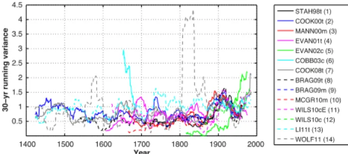
While there appears to be large-scale coherence among the reconstructed time series, the variance changes from these reconstructions differ considerably. For instance, half of the ENSO reconstructions (reconstruction numbers 1, 2, 3, 4, 6, 13 and 14 from Table 1) suggest that the ENSO variability recorded during the Little Ice Age (LIA,∼1550–1880) was
at times higher than reconstructions of most recent ENSO activity. The remaining reconstructions suggest that ENSO variability of the LIA failed to match recent levels. Thus, there is ambiguity among the reconstructions as to where current levels of ENSO variability are placed in the context of the past ∼600 yr, which reduces our confidence in how well any individual reconstruction can in fact capture low-frequency ENSO variance modulations.
In this study we use two multi-century coupled general cir-culation model (CGCM) simulations to examine an assump-tion made implicitly by many paleo-reconstrucassump-tion studies – i.e., that a good temporal correspondence between a given climate variable and ENSO translates also into a high corre-lation between multi-decadal variance changes in this vari-able and in ENSO (e.g., McGregor et al., 2010; Wilson et al., 2010; Li et al., 2011, 2013). We also test a simple method to extract the common ENSO variance modulation signal us-ing proxies from a variety of ENSO-teleconnected locations that is robust against small dating errors, unlike previous proxy analyses. We then use this method to identify the com-mon variance signal in a number of pre-defined proxy-based ENSO reconstructions and a range of single-station rainfall and temperature proxies over the past 600 yr.
2 Simulations
The CGCM simulations used in this study are the externally forced last-millennium (850–1850) simulation of the Com-munity Climate System Model, version 4 (hereafter CCSM4, Landrum et al., 2013), and a 2000 yr pre-industrial control run of the Geophysical Fluid Dynamics Laboratory (GFDL)-CM2.1 model with no changes in external forcings (Witten-berg, 2009). Note that prior to any analysis, annual mean (July–June) values of model precipitation and surface tem-perature (TS)data from the model simulations are calculated, and the resulting time series are filtered with a 10 yr high-pass Butterworth filter to isolate the variability in the classi-cal ENSO band of 2–8 yr.
It is noted that the experimental design differs between these two coupled model simulations: the CCSM4 sim-ulation includes estimates of observed time-varying forc-ing, such as solar, volcanic aerosols, and greenhouse gases, whereas CM2.1 includes these external forcings fixed at 1860
25
1400 1500 1600 1700 1800 1900 2000
0.5 1 1.5 2 2.5 3 3.5 4 4.5
Year
30−yr
running
variance
STAH98t (1) COOK00t (2) MANN00m (3) EVAN01t (4) EVAN02c (5) COBB03c (6) COOK08t (7) BRAG09t (8) BRAG09m (9) MCGR10m (10) WILS10cE (11) WILS10c (12) LI11t (13) WOLF11 (14)
Fig. 1.The running variance of each of the 10 yr high-pass-filtered ENSO reconstructions (reconstruction names and numbers corre-spond to those in Table 1). Note the individual reconstruction time series were normalized over the period 1900–1977 prior to calcu-lating the running variance in a 30 yr sliding window. Each running variance time series is then adjusted by adding a constant, such that their mean running variance over the period 1900–1977 matches that of the observed ENSO signal (defined as high-pass-filtered sur-face temperature averaged over the Niño 3.4 region) over the same period.
levels. However, we expect the results of this multi-model analysis to establish the robustness of the results presented in this manuscript, as the study of Landrum et al. (2013) has demonstrated that the addition of last-millennium time-varying forcing’s had no significant impact on the various internal modes of simulated climate variability in CCSM4 (e.g., ENSO, the North Atlantic Oscillation, Pacific Decadal Oscillation).
The atmospheric component of the CCSM4 simulation uses a uniform horizontal resolution of 1.258 in latitude by 0.98 in longitude, and has 26 layers in the vertical (Neale et al., 2013). The ocean model, which is based on version 2 of the Parallel Ocean Program model (Smith et al., 2010), uses the standard ocean grid with a displaced grid North Pole, nominal 1◦
horizontal resolution (uniform 1.18 in lon-gitude, variable in latitude from 0.27◦
at the Equator to 0.54◦
at 33◦
latitude), and 60 levels in the vertical (Danabasoglu et al., 2012). The land surface model adopts the same hori-zontal resolution as CAM4, while the sea ice model uses the same horizontal grid as the ocean component (Landrum et al., 2013). CCSM4’s simulation of tropical Pacific climate is described extensively in Deser et al. (2012). The seasonal evolution, phase asymmetry and teleconnections of the mod-eled ENSO are consistent with observations.
The CM2.1 ocean model is based on Modular Ocean Model version 4 (MOM4) code, with 50 vertical levels and a 1◦
×1◦
horizontal resolution that telescopes to 1/3◦
merid-ional spacing near the Equator. The atmospheric component has 24 vertical levels, 2◦
latitude by 2.5◦
Table 1.Existing ENSO reconstructions employed in this study. Note that these ENSO reconstructions have at least annual resolution and are pre-screened such that they have a correlation of at least 0.5 with the annual mean (July–June) observations of ENSO, represented by Niño
3.4 area-averaged (5◦S–5◦N, 120◦W–170◦W) SST anomalies (SSTA; Table 2). This correlation cutoff ensures the ENSO reconstruction
provides a skillful estimate of ENSO variability, at least over the instrumental epoch.
No. Label Reference Period Proxy type Source region
1 STAH98t Stahle et al. (1998) 1706–1997 Tree ring Pacific Basin
2 COOK00t Cook (2000) 1408–1978 Tree ring North America
3 MANN00m Mann et al. (2000) 1650–1990 Mixed Near global (tropics)
4 EVAN01t Evans et al. (2001) 1590–1990 Tree ring America
5 EVAN02c Evans et al. (2002) 1800–1990 Coral Indo-Pacific Basin
6 COBB03c Cobb et al. (2003) 1635–1703 & 1886–1998 Coral Central equatorial Pacific
7 COOK08t Cook et al. (2008) 1300–1978 Tree ring North America
8 BRAG09t Braganza et al. (2009) 1525–1982 Tree ring Pacific Basin
9 BRAG09m Braganza et al. (2009) 1727–1982 Mixed Pacific Basin
10 MCGR10m McGregor et al. (2010) 1650–1977 Mixed Near global (tropics)
11 WILS10cE Wilson et al. (2010) 1850–1998 Coral Eastern equatorial Pacific
12 WILS10c Wilson et al. (2010) 1540–1998 Coral Indo-Pacific Basin
13 LI11t Li et al. (2011) 900–2002 Tree ring North America
14 WOLF11 Wolff et al. (2011) 1208–2005 Lake varves East Africa
characterized by periods between 2 and 5 yr. SST anoma-lies in the eastern equatorial Pacific are skewed toward warm events, consistent with observations. The evolution of ENSO subsurface temperatures is also realistically represented, as are ENSO’s teleconnections. Tropical climate variability in CM2.1 is extensively described in Wittenberg et al. (2006), Capotondi et al. (2006), Kug et al. (2010), and Karamperidou et al. (2013).
3 Methods
3.1 Testing the running variance implications of a good temporal correlation
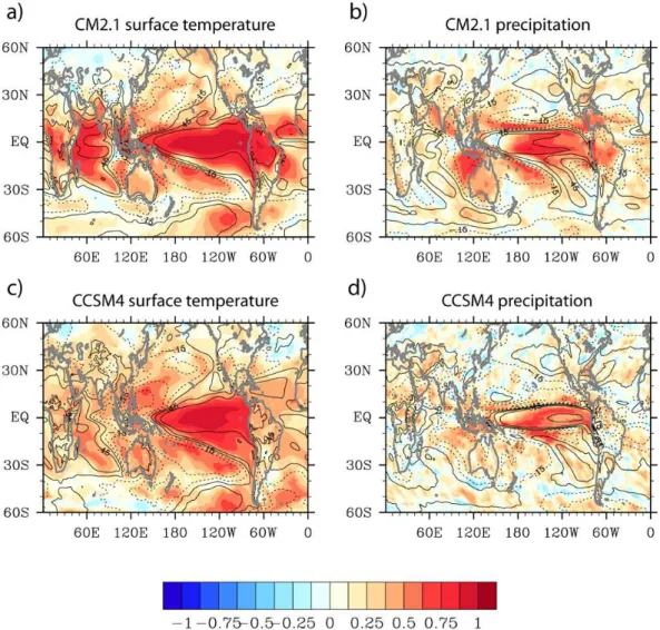
The fact that there is such a wide spread between the running variances of the individual ENSO reconstructions (Fig. 1) raises the question whether a good temporal correspondence between a given regional climate variable and ENSO can be used to imply that the variable will also provide a good repre-sentation of ENSO variance. We use output from the CCSM4 and CM2.1 models to address this question. The correla-tion between the simulated running variance ofTSin CM2.1 and the running variance of Nino 3.4 area-averaged (5◦S–
5◦N, 120◦W–170◦W) T
S anomalies, hereafter referred to as ENSO running variance (Fig. 2a, shading), is quite sim-ilar to the correlation between the simulatedTS and ENSO (Fig. 2a, contours). Note that to focus on ENSO’s multi-decadal changes the running variance in this study is cal-culated using a 30 yr sliding window. The pattern correla-tion between these two correlacorrela-tion maps amounts to 0.79 (r2=0.63). Similar results are also obtained for the CCSM4 simulation (comparing Fig. 2c contours versus shading). The corresponding pattern correlation is 0.70 (r2=0.49). In this
modeling framework, our results suggest that a large abso-lute value of the correlation betweenTSand ENSO provides a clear indication that the running variance ofTSwill track that of ENSO.
However, calculating the correlation between the CM2.1 simulated precipitation running variance with ENSO running variance (Fig. 2b, shading), and comparing this with the ab-solute value of the correlation between the simulated precipi-tation and ENSO (Fig. 2b, contours) reveals some key differ-ences in the tropical Pacific. For example, in the western trop-ical Pacific the correlation between precipitation and ENSO is high, with values falling between the 0.45 and 0.75 con-tours. However, the correlation between precipitation run-ning variance and ENSO runrun-ning variance in this region is near zero and even slightly negative, indicating that an in-crease in ENSO variance may be totally missed, or even dis-played as a decrease in variance, by precipitation in this re-gion. Similar differences are also seen for the CCSM4 sim-ulation (comparing Fig. 2d shading versus contours). We obtain pattern correlations between the temporal correlation maps of CM2.1 (i.e., comparing the shading versus contours in Fig. 2b) and CCSM4 (i.e., comparing the shading versus contours in Fig. 2d) that attain values of 0.67 (r2=0.45) and 0.55 (r2=0.31), respectively.
Fig. 2.Correlation between the running variance of the(a)simulated surface temperature (TS)and(b)precipitation running variance with
the running variance of the simulated ENSO index (defined as the area-averagedTSin the Niño 3.4 region) in CM2.1. The overlying contours
in panels(a)and(b)represent the correlations between simulatedTSand rainfall, respectively, with the simulated ENSO index. Contours
are from−0.75 to 0.75 with a spacing of 0.3 and negative contours are dashed.(c)and(d)as in(a)and(b), respectively, but for CCSM4
model output.
does not guarantee a strong correlation between the precip-itation running variance at that location and ENSO running variance. For instance, in CM2.1 if a simulated precipitation signal is selected that has anr2value of between 0.6 and 0.7 when compared with the simulated ENSO, there is a 10 % chance that the precipitation running variance time series has an r2< 0.1 (r< 0.31) when compared with ENSO running variance (Fig. 3a). This indicates either that (i) ENSO may influence the sign and timing of the rainfall change at this location – however, unrelated processes influence the mag-nitude of that change – or that (ii) the relationship between precipitation and ENSO at that location is highly non-linear. We find that a strong correlation between a common pre-cipitation time series, identified by calculating the median time series from multiple simulated precipitation time series
1
2 3
0 0.2 0.4 0.6 0.8 1
[0.2−0.3] [0.3−0.4] [0.4−0.5] [0.5−0.6] [0.6−0.7] > 0.7 0
0.2 0.4 0.6 0.8
Squared Correlation Coefficient (Common signal Vs ENSO)
Squared Correlation Coefficient
(Common
signal
RV
Vs
ENSO
RV)
0.1 0.2 0.3 0.4 a)
b)
Normalised Count
0 95%
5% 50% 95% 5% 50%
Fig. 3. (a)displays the 5 % (dashed lines), 50 % (solid lines) and 95 % (dash-dot lines) of squared correlation coefficients calculated between CM2.1 simulated precipitation running variance (calcu-lated in a 30 yr sliding window) and ENSO running variance, binned
on thexaxis against the squared correlation between the simulated
precipitation and ENSO. The color of the lines indicates the number of source locations utilized in the precipitation signal, with black, blue and red lines corresponding to one, two and five source loca-tions. The inset histogram displays the distribution of squared cor-relation coefficients calculated between precipitation running
vari-ance and ENSO running varivari-ance from thexaxis bin of the main
plot shaded grey.(b)as in(a)but for CCSM4 model output. Note
the differentyaxis for panels(a)and(b).
will make it 3.5 times less likely that the common precipi-tation running variance will have anr2< 0.1 (r< 0.31) when compared with ENSO running variance (Fig. 3b).
Thus, these results suggest the following: (i) a strong cor-relation betweenTS and ENSO provides a clear indication that the running variance of TS is likely to track that of ENSO; (ii) a strong correlation between precipitation and ENSO at a particular location does not guarantee a strong correlation between the running variance of precipitation and the running variance of ENSO. As such, ENSO variance es-timates provided by reconstructions derived from precipita-tion sensitive proxies at a single site should be viewed with caution; and (iii) a multi-site common precipitation signal which is strongly correlated with ENSO provides much bet-ter indication that the common precipitation signal’s running variance will be related to the running variance of ENSO.
3.2 Identifying the common variance signal
A previous study has shown that a linear combination of many of the above-listed individual eastern equatorial Pacific reconstructions can further increase the signal-to-noise ratio compared with the individual reconstructions (McGregor et al., 2010). However, it was noted that the variance changes of this combined proxy product appeared to show the effects of dating errors towards the beginning of the 350 yr record. Sim-ilar dating errors have also been noted in studies that attempt to reconstruct observed ENSO over the last 1000 yr (Emile-Geay et al., 2013a, b). This is a concern because proxies dis-playing small dating errors can act to cancel out the common signal when combined – hence artificially reducing the com-bined signal variance.
3.2.1 Methods for identifying the common variance signal
McGregor et al. (2010) proposed that working with the run-ning variance proxy time series should provide a more ro-bust estimate of ENSO’s variance changes in the presence of small dating errors than working with raw proxy time series. This is because small dating errors in proxies can act to cancel out the common signal in the 2–8 yr variabil-ity range when combined, acting to artificially reduce the combined signal variance, while the positive definiteness of the running variances precludes this signal cancellation. This is further tested by examining whether identifying the me-dian of the running variance signals (MRV) of numerous source proxies (e.g., median (σ2(Px(t )))) is equivalent to
identifying the running variance of the median signal (RVM) (e.g., σ2(median (Px(t ))) in the absence of dating errors.
The source proxy time series are abbreviated asPx(t ). Thus,
MRV refers to calculating the running variance for each individual proxy, and then finding the inter-proxy median; whereas RVM refers to the finding the inter-proxy median of the individual time series first, and then calculating the run-ning variance of that common signal.
To assess the performance of these two methods in the ab-sence of dating errors, we analyze the output of the CCSM4 and CM2.1 multi-century model simulations. To this end, we selectx(x= 1, 2, 3, . . . , 14) time series of either precipitation orTSfrom random global locations, with the only constraint on the location being that its time series must have a absolute correlation coefficient > 0.3 when compared to the simulated ENSO (again note that ENSO is represented as area-averaged
TS in the Niño 3.4 region). We then calculate the MRV and RVM of thextime series. The running variance is calculated in a 30 yr sliding window. This procedure is repeated until we obtain 10 000 MRVs and 10 000 RVMs for eachx repre-senting either precipitation or surface temperature.
Table 2.Correlation coefficients calculated between the high-pass-filtered (HPF; 10 yr cutoff) annual mean proxy-network-based ENSO reconstructions and HPF observed ENSO during the overlapping instrumental period, along with the across observational product average displayed in bold font. All correlations are statistically significant above the 99 % level. We note that this measure of statistical signifi-cance takes into account serial (auto-)correlation in the series, based on the reduced effective number of degrees of freedom outlined by Davis (1976).
Observed ENSO (Niño 3.4 region SSTA)
HadISST ERSST V3 Kaplan Niño 3.4 SSTA
No. Label (Rayner et al., 2003) (Smith et al., 2008) (Kaplan et al., 1998) (Bunge and Clarke, 2009) Average
1 STAH98t 0.74 0.75 0.76 0.73 0.75
2 COOK00t 0.78 0.71 0.77 0.77 0.76
3 MANN00m 0.77 0.76 0.75 0.76 0.76
4 EVAN01t 0.54 0.69 0.55 0.59 0.59
5 EVAN02c 0.74 0.78 0.72 0.71 0.74
6 COBB03c 0.71 0.7 0.72 0.69 0.71
7 COOK08t 0.76 0.74 0.75 0.73 0.75
8 BRAG09t 0.63 0.58 0.59 0.64 0.61
9 BRAG09m 0.69 0.66 0.66 0.69 0.68
10 MCGR10m 0.83 0.83 0.82 0.82 0.83
11 WILS10cE 0.58 0.65 0.56 0.62 0.60
12 WILS10c 0.58 0.59 0.6 0.61 0.60
13 LI11t 0.53 0.48 0.55 0.54 0.53
14 WOLF11 0.54 0.57 0.54 0.58 0.56
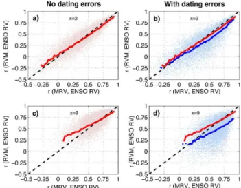
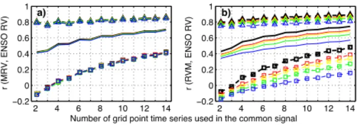
values calculated between ENSO running variance and the RVM, reveals that the percentiles of the two derivation meth-ods are very similar for both fields in both models (Fig. 4). This is also basically confirmed by plotting the ENSO run-ning variance and RVM correlation coefficients against the corresponding ENSO running variance and MRV correlation coefficients (Fig. 5a and c). What is also apparent from both of these panels, however, is that as the number of proxy lo-cationsx increases, the RVM outperforms the MRV for low correlation values (r< 0.5). For larger correlations though, the mean RVM/MRV correlations follow a one-to-one line reasonably well. The scatter seen in Fig. 5a and c indicates that both methods will provide somewhat different estimates of the ENSO running variance time series; however, in the absence of dating errors the MRV method is statistically comparable to the results of the RVM calculation.
Furthermore, we see that as the number of proxies (x) in-creases, the common signal is more likely to provide a skill-ful estimate of ENSO running variance. This confirms one of the initial assumptions used in many paleo-climate studies: that a network of proxies helps to reduce the effects of biases, noise, and weaknesses in the individual indicators (Mann et al., 2000).
3.2.2 Effects of dating errors on the common running variance signal
Here we examine whether calculating the MRV (calculating the running variance for each individual proxy, and then find-ing the inter-proxy median), as opposed to calculatfind-ing the RVM (finding the inter-proxy median of the individual time
series first, and then calculating the running variance of that common signal), alters the effects of dating uncertainties in the reconstructions of ENSO variance. As discussed above, McGregor et al. (2010) proposed that working directly with the running variance time series, as opposed to the raw time series, acts to reduce the effects of dating uncertainties by not allowing slightly shifted signals to damp out the common signal variance. To this end, five sets of precipitation time se-ries are extracted from the CM2.1 simulation, which include all precipitation time series that have the absolute value of the correlation coefficients > 0.3 with simulated ENSO. In four of these five sets, a fraction of the entire time series is ran-domly shifted temporally by 1–5 yr to mimic a dating error. What varies between these four sets, however, is the propor-tion of the time series that is subject to the introduced dating error, changing from 1/5, 1/4, 1/3, and 1/2. Thus, of these four precipitation data sets the first has dating errors of be-tween 1 and 5 yr introduced into 1/5 of all time series, the second has dating errors introduced into 1/4 of all time se-ries, and so on.
Using these data and the approach outlined above in Sect. 3.2.1, we select x (x= 1, 2, 3, . . . , 14) precipitation time series from one of these data sets and then calculate the MRV and RVM. The 5th, 50th and 95th percentiles of the correlations calculated between ENSO running variance and the MRV for each of the five data sets as a function ofx
2 4 6 8 10 12 14 ï0.2
0 0.2 0.4 0.6 0.8 1
2 4 6 8 10 12 14 ï0.2
0 0.2 0.4 0.6 0.8 1
2 4 6 8 10 12 14 ï0.2
0 0.2 0.4 0.6 0.8 1
2 4 6 8 10 12 14 ï0.2
0 0.2 0.4 0.6 0.8 1
Number of grid point time series used in the common signal
Common signal RV correlation with ENSO RV
b)
d) c)
a) CM2.1 surface temperaure CM2.1 precipitation
CCSM4 precipitation CCSM4 surface temperaure
Fig. 4. (a)The 5 % (dashed line with squares), 50 % (solid line) and 95 % (dashed lines with triangles) of the correlation coefficients
cal-culated between the CM2.1 simulated MRVTSand ENSO running
variance are displayed in red, while those of the CM2.1 simulated
RVMTSand ENSO running variance are displayed in black.(b)as
in(a)but for the CM2.1 precipitation data.(c)and (d) as in(a)
and(b)but for CCSM4TSand precipitation data, respectively. The
xaxis in each panel displays the number of grid point time series
used to calculate the common signal.
between ENSO running variance and the RVM signal reveals that the introduced dating errors have a large effect on the es-timates of running variance identified by the RVM method (Fig. 6b). This is further illustrated by plotting ENSO run-ning variance and the RVM against the corresponding ENSO running variance and MRV correlation coefficients, both with dating errors introduced in 1/2 of all time series incorporated in the median signals, and comparing this with correspond-ing values with no introduced datcorrespond-ing errors (Fig. 5b and d). The results clearly indicate that the MRV method provides a much more robust estimate of ENSO’s running variance than the RVM method when dating errors are present in the input time series. We note that this result remains consistent re-gardless of the model (CM2.1 or CCSM4) or the output field used (i.e., precipitation orTS).
4 Application to existing ENSO proxy reconstructions
Here we examine the MRV (calculating the running variance for each individual proxy, and then finding the inter-proxy median) of the 14 existing ENSO reconstructions listed in Table 1 and presented in Fig. 11. Each of these reconstruc-tions is based on current and paleo-proxy data sources from a range of geographic regions, with a variety of statistical
1The term “existing ENSO reconstructions” refers to ENSO
re-constructions (see Table 1) that have been previously defined in the scientific literature. These reconstructions often use proxy data from multiple locations and rely on statistical methods to extract the ENSO signal.
Fig. 5. (a)The correlation between CM2.1 rainfall MRV and ENSO (defined as the area-averaged SSTA in the Niño 3.4 region) run-ning variance plotted against the correlation between CM2.1 rainfall RVM and ENSO running variance for the case with only two
mem-bers (x=2). Panel(c)displays the same fields, however in this case
x=9. The solid red line in both of these panels represents the mean
correlation of ther(RVM,ENSO RV) in bins of width 0.025 along
thexaxis.(b)and(d)as in(a)and(c)but 1/2 of all rainfall time
series include an introduced temporal shift to mimic a proxy dating error. In both of these panels the solid blue line represents the mean
correlation of ther(RVM,ENSO RV) calculated in bins with width
0.025, while the solid red lines in panels(b)and(d)are mean RVM
value from panels(a)and(c), respectively (i.e., those with the same
xand no introduced dating error). Note, the black dashed line in
all panels represents the one-to-one line, while the mean values are only plotted when the bin contains a minimum of 20 RVM values.
methods used in the derivation of the relevant indices (see Table 1 and references therein). Considering that we have shown that the multi-proxy approach minimizes the impact of weaknesses in any individual proxy (Sect. 3.2.1), it is ex-pected that the use of this wide network of ENSO proxies will allow us to reconstruct the long-term changes in past ENSO variance with greater statistical skill than available from individual reconstructions alone.
2 4 6 8 10 12 14 ï0.2
0 0.2 0.4 0.6 0.8 1
Number of grid point time series used in the common signal
r (MRV, ENSO RV)
2 4 6 8 10 12 14
ï0.2 0 0.2 0.4 0.6 0.8 1
r (RVM, ENSO RV)
b) a)
Fig. 6. (a)The 5 % (dashed line with squares), 50 % (solid line) and 95 % (dashed lines with triangles) of the correlation coefficients cal-culated between the CM2.1 rainfall MRV and ENSO running
vari-ance, while(b)displays the percentiles of correlation coefficients
calculated between CM2.1 rainfall RVM and ENSO running vari-ance. The black lines indicate those percentiles using data with no introduced dating errors, while the red, yellow, green and blue line respectively represent those percentiles using data with 1/5, 1/4, 1/3, 1/2 of the time series including an introduced dating error.
2009). As in the models, the observed ENSO is represented as area-averaged temperature in the Niño 3.4 region and for consistency with the reconstructions it has been filtered with a 10 yr high-pass Butterworth filter. The large spread between the running variances, shown in Fig. 1, highlights the dis-crepancies amongst the ENSO reconstruction variances (see also grey dots in Fig. 7).
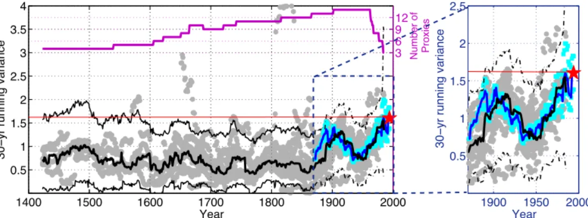
Comparing the MRV of the ENSO reconstructions with the MRV of the observed ENSO over the instrumental pe-riod reveals a remarkable correspondence (Fig. 7). The swing from high variance in the earliest decades of the 20th cen-tury to low variance in the middle of the 20th cencen-tury and an increasing trend thereafter are well reproduced in the recon-struction MRV. Note that the MRV of the observed ENSO is calculated across 4 available observational estimates (Ta-ble 2). The correspondence between observations and recon-structions further increases the confidence in the MRV tech-nique applied here. Figure 7 also reveals that the amplitude of the observed MRV in the most recent 30 yr of the 20th cen-tury (1979–2009, indicated by the red star) appears to have been larger than the variance in any 30 yr window during the preceding multi-century reconstruction MRV record.
We note that the number of ENSO reconstructions taken into account when calculating its MRV signal varies with time, depending on the length and span of the individual records (Fig. 7, Table 1). Error bars are calculated using two separate pseudo-proxy methods, such that the length of the error bar varies in relation to the number of available ENSO proxies (see Appendix A). For instance, with fewer ENSO reconstructions available (e.g., during the period 1400–1500) the running variance estimate becomes more uncertain than for a period (e.g., the 1800s) where many more ENSO restructions are available. At any point in time the most con-servative (widest) error bar of the two pseudo proxy methods (Appendix A) is displayed in Fig. 7.
The increased variance of observed ENSO for the most recent 30 yr is significantly larger (exceeding the 95 %
confidence level) than for any 30 yr interval during the pe-riod 1590–1880 (i.e., the observed variance, indicated by the red star, is larger than the ENSO reconstruction MRV error bars in the period from the year 1590 through to the start of the instrumental data). Prior to 1590, however, the uncer-tainty range of the MRV signal, estimated by the error bars, is too large to be conclusive.
4.1 Independence of existing ENSO proxy reconstructions
We note that some of the input proxy networks overlap among these 14 ENSO reconstructions (see Appendix B for a more in-depth discussion), such that they are not always completely independent in a geographical sense. In spite of the geographical overlap for some of the reconstructions, usually different statistical methods are applied to tease out the ENSO signal. These methods range from calculating an empirical orthogonal function (EOF) of the input proxy net-work (e.g., Braganza et al., 2009; McGregor et al., 2010; Li et al., 2011) to the more complex method of regressing proxy data onto the leading spatio-temporal eigenmodes of observed data (e.g., Mann et al., 2000; Evans et al., 2002; Cook et al., 2008).
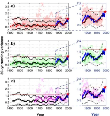
Despite the methodological differences, this lack of in-dependence raises the concern that the noise, i.e., the non-ENSO component of these overlapping input proxies, may distort or mask the common ENSO signal and this could be incorrectly attributed to changes in ENSO. If this were true, we would expect the noise influencing tropical coral-dependent reconstructions to be distinct from that of North American tree rings. As such, if the running variance of either or both of these groups’ reconstructions were dom-inated by noise, we would expect to see significant differ-ences in their common variance signal. However, this is not the case. Identifying the common variance signal in only those reconstructions with common tropical corals reveals a post-1700 signal that is extremely similar to that identified in only those reconstructions with common North American tree rings (Fig. 8). In addition, both of the above signals re-semble the MRV identified from the full set of ENSO recon-structions. This gives us confidence that the MRV identified in this study is not strongly distorted or dominated by ENSO-independent noise. We note that reconstructions 3 and 9 in-clude common tropical corals and North American tree rings; however, neglecting these two reconstructions from both of the above subsets leaves the common variance signals virtu-ally unchanged (figure not shown).
5 Application to observed single-station proxies
31 1
Figure 7: The running variance (grey dots) of each of the 14 ENSO reconstructions, overlaid 2
3
1400 1500 1600 1700 1800 1900 2000
0.5 1 1.5 2 2.5 3 3.5 4
Year
30
ï
yr running variance
3 6 9 12
Number of Proxies
1900 1950 2000
0.5 1 1.5 2 2.5
Year
30
ï
yr running variance
Fig. 7.The running variance (grey dots) of each of the 14 ENSO reconstructions, overlaid with the MRV (thick black line). At any point in time prior to the observation period, the thin black lines represent the widest median running variance signal error bars of the two types of error analysis detailed in Appendix A. Inside the window of instrumental data these error bars change to thin black dash-dot lines, as we have a direct measurement of ENSO variance. The width of each of these two error bar estimates varies depending on the number of ENSO variance proxies available (see purple line at top of panel). Cyan dots indicate the running variance of 4 different estimates of observed ENSO (Table 2), while the blue line represents the MRV of these observed ENSO running variance time series. The red star indicates the most recent value of the observed MRV, while the thin red line just extends this most recent value back through time, for comparison with the ENSO reconstruction MRV and its error bars.
the common information contained within these reconstruc-tions rather than defining another reconstruction to add to the literature. However, as the ENSO reconstructions in most cases have already incorporated information from numerous time series, artificial variance reduction due to dating errors in the source proxies may already be incorporated into our analysis. As such, we may not be getting the best out of the methodological advantage of combining running variances when applying it to these synthesized time series.
Thus, here we also examine the MRV signal in a range of single-location proxies from either within or surrounding the Pacific Basin and compare the results with those derived above (Table 3). Again we focus on the interannual ENSO frequency by filtering each of the proxy time series with a 10 yr high-pass Butterworth filter. We utilize all tree ring proxies listed by Emile-Geay et al. (2013a, b) and all tropical Pacific coral proxies available from the NOAA National Cli-mate Data Center (NCDC) that continuously span the period 1800–1980. Use of this time period ensures that all included proxies provide at least 50 yr of information prior to the start of observed estimates of SST, which start between 1854 and 1886. However, prior to their inclusion in Table 3, these prox-ies were pre-screened to ensure they have a correlation of at least 0.3 when compared with observed ENSO (Table 4). Each of these filtered proxy time series are then normalized over the 1900–1977 period, and a time series of running vari-ances, in a thirty-year sliding window, is calculated for each reconstruction. The variance time series are then adjusted by adding a constant, such that their mean running variance over the period 1900–1977 matches that of observed ENSO over the same period.
1 2 3
14000 1500 1600 1700 1800 1900 2000 1
2 3
14000 1500 1600 1700 1800 1900 2000 1
2 3
30−yr
running
variance
Year a)
b)
STAH98t (1) COOK00t (2)
MANN00m (3)
EVAN01t (4) COOK08t (7)
BRAG09t (8)
BRAG09m (9) LI11t (13)
MANN00m (3)
EVAN02c (5)
COBB03c (6) BRAG09m (9)
WILS10cE (11)
WILS10c (12)
Fig. 8. (a)The running variance of each of the 8 ENSO reconstruc-tions with common tree ring source proxies (proxy names and num-bers correspond to those in Table 1), overlaid with the
correspond-ing MRV (thick dashed red line).(b)The running variance of each
of the 6 ENSO reconstructions with common tropical coral recon-structions (proxy numbers in legend correspond to those in Table 1), overlaid with the corresponding MRV (thick dashed red line). The underlying thick black line in both panels represents the MRV of all 14 ENSO reconstructions presented in Fig. 7 and Table 1, while the thin black lines represent the accompanying ENSO reconstruc-tion MRV signal error bars (Appendix A). The red star indicates the most recent value of the observed MRV (see Fig. 7).
Table 3.The single station (SS) temperature and/or rainfall proxies employed in this study. Note that these proxies have at least annual resolution and are pre-screened such that they have a correlation of at least 0.3 with the annual mean (July–June) observations of ENSO,
represented by Niño 3.4 area-averaged (hereafter N34, 5◦S–5◦N, 120◦W–170◦W) SST anomalies (Table 4). This correlation cutoff ensures
that the proxies provide a reasonably skillful estimate of ENSO variability over the instrumental epoch.
Reference Period Proxy type Location Source region Lat Lon
SS proxy 1 Cook et al. (2008) 0–2006 Tree ring width NADA PDSI North America 27◦N 255◦E
SS proxy 2 Le Quesne et al. (2006) 1000–2000 Tree ring width Chilean Cordillera South America 33◦S 288◦E
SS proxy 3 ITRDB extraction 1675–1998 Tree ring width Madera Canyon Mexico 29◦N 257◦E
SS proxy 4 ITRDB extraction 1553–1998 Tree ring width Nevado de Colima Mexico 20◦N 256◦E
SS proxy 5 ITRDB extraction 1376-1998 Tree ring width Cerro Baraja Mexico 26◦N 254◦E
SS proxy 6 ITRDB extraction 1376-1999 Tree ring width Cerro Baraja Mexico 26◦N 254◦E
SS proxy 7 ITRDB extraction 1644-1998 Tree ring width Creel Int. Airport Mexico 28◦N 252◦E
SS proxy 8 ITRDB extraction 1481–1998 Tree ring width El Salto Mexico 24◦N 254◦E
SS proxy 9 ITRDB extraction 1583–1998 Tree ring width El Tabacote/Tomochic Mexico 28◦N 252◦E
SS proxy 10 ITRDB extraction 1712–1998 Tree ring width Capote Knob Texas, USA 29◦N 262◦E
SS proxy 11 ITRDB extraction 1473–1998 Tree ring width Camp Spring Texas, USA 29◦N 257◦E
SS proxy 12 ITRDB extraction 1473–1998 Tree ring width Camp Spring Texas, USA 29◦N 257◦E
SS proxy 13 Asami et al. (2005) 1790–2000 Coral (δ18O) Double Reef Guam 13◦N 144◦E
SS proxy 14 Bagnato et al. (2005) 1776–2001 Coral (δ18O) Savusavu Bay Fiji 16◦S 179◦E
SS proxy 15 DeLong et al. (2012) 1648–2000 Coral (Sr/Ca) Amédée Island New Caledonia 22◦S 166◦E
SS proxy 16 Isdale et al. (1998) 1644–1986 Coral (Fluorescence) Havannah Island Great Barrier Reef 18◦S 146◦E
SS proxy 17 Isdale et al. (1998) 1737–1980 Coral (Fluorescence) Pandora Reef Great Barrier Reef 18◦S 146◦E
SS proxy 18 Linsley et al. (2000) 1727–1997 Coral (Sr/Ca) Rarotonga Cook Islands 21◦S 159◦W
SS proxy 19 Lough (2007) 1631–2005 Coral (Fluorescence) Queensland River Flow Great Barrier Reef 17–23◦S 146–151◦E
SS proxy 20 Quinn et al. (1998) 1657–1992 Coral (δ18O) Amédée Island New Caledonia 22◦S 166◦E
SS proxy 21 Charles et al. (2003) 1782–1990 Coral (δ18O) Lombok Straight Indonesia 8◦S 115◦E
Table 4.Correlation coefficients with zero lag, and lead and lag times of one year (t−1 means proxy data lagging observed ENSO), calculated between the high pass filtered (HPF; 10 yr cutoff) annual mean single station proxy network (Table 3) and the annual mean (July–
June) observations of ENSO, represented by Niño 3.4 area-averaged (5◦S–5◦N, 120◦W–170◦W) SST anomalies during the overlapping
instrumental period. The maximum correlation for each observational product is highlighted by bold font.
Observed Niño 3.4 region SSTA
HadISST HadISST HadISST Niño 3.4 SSTA
(Rayner et al., 2003) (Smith et al., 2008) (Kaplan et al., 1998) (Bunge and Clarke, 2009)
t−1 t t+1 t−1 t t+1 t−1 t t+1 t−1 t t+1
SS proxy 1 0.12 −0.61 0.18 0.10 −0.62 0.23 0.11 −0.61 0.14 0.09 −0.61 0.20
SS proxy 2 −0.04 0.29 −0.19 0.06 0.21 −0.26 −0.04 0.30 −0.17 −0.03 0.26 −0.17
SS proxy 3 −0.25 0.43 −0.01 −0.21 0.45 −0.05 −0.21 0.41 0.00 −0.21 0.44 0.00
SS proxy 4 −0.01 0.32 −0.09 −0.14 0.31 0.02 −0.02 0.33 −0.08 0.00 0.29 −0.13
SS proxy 5 −0.33 0.43 −0.05 −0.29 0.42 −0.16 −0.32 0.40 −0.04 −0.29 0.43 −0.08
SS proxy 6 −0.33 0.46 −0.07 −0.30 0.44 −0.18 −0.33 0.42 −0.06 −0.30 0.45 −0.10
SS proxy 7 −0.21 0.43 −0.19 −0.23 0.41 −0.24 −0.20 0.40 −0.15 −0.19 0.41 −0.19
SS proxy 8 −0.24 0.55 −0.11 −0.14 0.47 −0.19 −0.22 0.48 −0.09 −0.20 0.50 −0.13
SS proxy 9 −0.27 0.49 −0.12 −0.26 0.50 −0.22 −0.25 0.47 −0.09 −0.25 0.48 −0.14
SS proxy 10 −0.27 0.24 0.07 −0.28 0.33 0.02 −0.27 0.22 0.09 −0.22 0.26 0.04
SS proxy 11 −0.24 0.40 0.01 −0.22 0.45 −0.08 −0.22 0.38 0.03 −0.23 0.42 −0.02
SS proxy 12 −0.23 0.38 0.03 −0.21 0.47 −0.11 −0.20 0.37 0.03 −0.20 0.39 0.00
SS proxy 13 0.43 0.04 −0.09 0.53 0.10 −0.10 0.38 0.07 −0.11 0.43 0.07 −0.07
SS proxy 14 0.59 0.24 −0.34 0.65 0.23 −0.37 0.57 0.26 −0.30 0.58 0.26 −0.32
SS proxy 15 −0.03 −0.50 −0.16 −0.04 −0.45 −0.14 −0.01 −0.47 −0.15 −0.06 −0.48 −0.12
SS proxy 16 −0.42 0.14 0.30 −0.34 0.10 0.28 −0.40 0.13 0.31 −0.38 0.21 0.24
SS proxy 17 −0.34 0.15 0.30 −0.21 0.14 0.23 −0.30 0.18 0.27 −0.26 0.22 0.21
SS proxy 18 −0.07 −0.44 0.03 −0.18 −0.50 0.15 −0.09 −0.43 0.02 −0.08 −0.44 0.03
SS proxy 19 −0.30 0.08 0.24 −0.30 0.05 0.27 −0.30 0.12 0.28 −0.26 0.15 0.20
SS proxy 20 0.15 0.28 −0.06 0.25 0.18 −0.04 0.15 0.26 −0.05 0.15 0.31 −0.07
Fig. 9. (a)The running variance (pink dots) of each of the 21 single-station proxies (Table 3) overlaid with their MRV (thick dashed red
line).(b) The running variance of the 12 single-station tree ring
proxies (light green dots) overlaid with the corresponding MRV
(thick green dashed line), while(c)displays the running variance
of the 9 single-station coral proxies (light purple dots) overlaid with the corresponding MRV (thick purple dashed line). The thick black line in all three panels represents the MRV of all 14 HPF (10 yr cut-off) ENSO reconstructions presented in Fig. 7 and Table 1, while the thin black lines represent the accompanying ENSO reconstruc-tion MRV signal error bars (Appendix A). As in Fig. 7, the blue line represents the MRV of observed ENSO and the red star indicates its most recent value, while the thin red line just extends this most recent value back through time for comparison with the proxy MRV signals.
series presented in Sect. 4.1 and Fig. 7. In fact, compar-ing the scompar-ingle-station proxy MRV time series with that of the MRV ENSO reconstruction reveals a strong similarity through most of the 600 yr period (Fig. 9a).
Using only the 12 single-station tree ring proxies (sourced from Emile-Geay et al., 2013; Table 3) we calculate the MRV signal. Comparing this single-station tree ring MRV signal with the MRV of the observed ENSO reveals a good cor-respondence (Fig. 9b inset). Again, this single-station MRV time series falls well within the error estimates of the ENSO reconstruction MRV time series, and directly comparing this single-station MRV time series with that of the ENSO recon-struction MRV time series reveals a strong similarity through most of the 600 yr period (Fig. 9b).
Calculating the MRV signal of the 9 coral proxies from Table 3, and comparing this with the MRV of the ob-served ENSO, reveals some correspondence (Fig. 9c inset),
although the correlation appears much weaker than for the single-station tree ring MRV (Fig. 9b inset). The correspondence is most notable prior to 1960; after this time the MRV of observed ENSO begins to steadily increase while the single-station coral proxy MRV signal remains relatively constant. The facts that (i) the single-station coral proxy MRV does not pick up the increase in ENSO variance since the mid-1900s, and that (ii) there is very little correspondence between the single-station coral proxy MRV and the ENSO reconstruction MRV time series outside of the period 1850– 1950 (Fig. 9c), reduces our confidence in this signal, which is namely sourced from the southwestern tropical Pacific, as it relates to ENSO. As the southwestern tropical Pacific is home to the South Pacific Convergence Zone (SPCZ), a pos-sible explanation for these discrepancies could be that there may have been slow shifts in the tropical Pacific tempera-ture/rainfall covariance that could have affected some of the
δ18O-based coral proxies in this region. However, in spite of this, the coral common variance time series falls mostly within the error estimates of the ENSO proxy reconstruction MRV signal.
Thus, consistent with the analysis of existing ENSO recon-structions presented in Fig. 7, the MRV of the single-station proxies of Table 3 (whether they are based on all single-station proxies or solely on coral or tree ring single-single-station proxies) reveals that the observed variance of ENSO in the most recent 30 yr of the 20th century (indicated by the red star) appears to have been larger than at any time during the preceding multi-century record.
6 Discussion and conclusions
The main goal of this study was to synthesize existing ENSO reconstructions to arrive at a better estimate of past ENSO variance changes. This is an important task since there are considerable discrepancies in ENSO variance estimates de-rived from the 14 available ENSO reconstructions that ex-hibit good correlations with the instrumental data (Figs. 1 and 7 and Table 2). Throughout the manuscript variance changes in the 10 yr high-pass-filtered ENSO reconstructions were calculated in a 30 yr sliding window to capture multi-decadal variance changes. Sensitivity analysis suggests that the re-sults discussed here are not sensitive to the high-pass filtering or the running variance window length (not shown).
Thus, we recommend caution when inferring ENSO running variance from precipitation-sensitive proxy data from a ge-ographically confined area, even if the data originate from ENSO’s main activity region in the central/eastern equato-rial Pacific. Furthermore, we demonstrated that this effect is significantly reduced when a common precipitation signal is sourced from a range of geographic regions. That is, a com-mon precipitation signal, which is strongly correlated with ENSO, provides a much better indication that the correla-tion between the rainfall running variance and ENSO running variance will also be strong.
By focusing on the median of the running variances of in-dividual source signals in this study we considerably sim-plified the approach of McGregor et al. (2010), who uti-lized a principle component analysis (PCA) of running vari-ance time series. Our new method has two main advantages: (i) it can easily deal with discontinuous data, and (ii) it does not weight the contribution of individual proxies on the combined signal, which may make it less sensitive to changes in ENSO’s teleconnections over time.
Our model analysis then showed that in the absence of dat-ing errors, the MRV method (median runndat-ing variance, i.e., calculating the running variance for each individual proxy, and then finding the inter-proxy median) yields similar re-sults to the RVM (running variance of the median, i.e., find-ing the inter-proxy median of the individual time series first, and then calculating the running variance of that common signal) approach. However, MRV is much less sensitive to dating errors than RVM. This is because small dating errors in the proxy time series can act to cancel out the common signal when combined, acting to artificially reduce the com-bined signal variance; the positive definiteness of running variances prevents this signal cancellation.
The results of our model analysis also show that as the diversity of input proxies increases, the resulting common variance signal is more likely to provide a skillful estimate of ENSO running variance. This confirms one of the initial assumptions used in many paleo-climate studies: that a broad network of proxies helps to reduce the effects of biases and weaknesses in the individual indicators (Mann et al., 2000). Thus, we expect the MRV method to increase the signal-to-noise ratio of the ENSO variance changes, while minimizing the effects of dating uncertainties in the source proxies.
As such, we applied this method to synthesize the vari-ance information contained in 14 preselected ENSO recon-structions (Table 1), and in 21 single-station proxy records (Table 3). However, prior to summarizing the key results of this analysis, we discuss several important limitations of the modeling and proxy analyses presented in this study.
The model analysis presented in Sect. 3 includes several caveats. First, model biases in the mean state and ENSO teleconnections could produce biases in the spatial patterns of difference between anomaly and running variance corre-lations with ENSO. Second, mixed temperature and rainfall sensitivities of some proxies (e.g., Cobb et al., 2003) could
complicate the interpretation in Sect. 3.1; however, for real-world applications perhaps the most conservative interpre-tation of these results is that amulti-site reconstruction of ENSO variance provides a more robust indication of changes in ENSO signal running variance than single-site proxy re-constructions. Third, ENSO teleconnections might not truly be stationary; however, as we have been assessing our meth-ods against the modeled ENSO variability, at least any
sim-ulated changes in teleconnections would be implicitly
in-cluded in our analysis.
The proxy analyses presented in Sects. 4 and 5 also in-cludes several caveats. First, although our combined ance estimate (Sect. 4) is supported by the running vari-ance signal calculated from uncalibrated single-station corals (see Sect. 5), we do not assess the sensitivity of individual source ENSO reconstructions to their derivation and calibra-tion techniques. A recent study has suggested that recon-structed centennial-scale variability is particularly sensitive to the historical SST data set used during calibration (Emile-Geay et al., 2013a, b). Second, we assume that the spatial structure of ENSO SSTA and ENSO’s teleconnections do not change over time; this is a concern, as the single-station proxies (Table 3) are largely sourced from regions considered teleconnected to ENSO and do not include any proxies from ENSO’s center of action in the eastern/central tropical Pa-cific. While the common running variance signals of these single-station proxies support the synthesis of pre-defined ENSO reconstructions, the differences between the common running variance time series could reflect changes of telecon-nection patterns over time (Fig. 9b and c).
With these caveats in mind, our synthesis of the 14 pre-defined ENSO reconstructions (Table 1), along with the anal-ysis of 21 single-station proxy records (Table 3), suggests that the observed variance of ENSO over the period 1979– 2009 was larger than the variance in any 30 yr window from the preceding 600 yr. As a result of the larger error bars in the estimates for the period prior to 1590 CE, however, we cannot rule out that the levels of ENSO variance that oc-curred between 1400 and 1590 may be comparable to that of 1979–2009. The unusually high 20th-century ENSO vari-ance is consistent with our previous results (McGregor et al., 2010), with other studies based on multi-site tree ring recon-structions (Li et al., 2013) and with the recent coral studies of Hereid et al. (2013) and Cobb et al. (2013).
Appendix A
Error bar calculation
The main goal of this pseudo-proxy technique is to assess how accurately the median of multiple pseudo-proxies can estimate the variance of the original proxies from which the pseudo-proxies are generated. Here we define the orig-inal source proxy as the “true” signal. To this end, each of the 14 normalized high-pass-filtered proxy time series
pi(t )(i=1, . . . , 14) (Table 1) is used as a true signal.
Pseudo-proxiesppij(t )=pi(t )+szj(t )(j=1, . . . ,J;J=
600) are generated by adding Gausian white noise zj(t )
to the annual mean true signal. The variance of zj(t ) is
randomly modulated by s, such that the correlation co-efficient between the pseudo-proxy ppij(t ) and the
orig-inal proxy pi(t ) (the true signal) is contained within the
range of correlation coefficients between the original proxies and the instrumental SSTA signal (see Table 2). By def-inition, selecting numerous pseudo-proxies and averaging (mean (ppi(t ))=J−1zjppij(t )) should allow for the true
signalpi(t )to be identified, as the additive Gaussian white
noise would cancel out if enough pseudo-proxies were uti-lized. If none of the proxy records had dating errors, the 30 yr running variance of mean (ppi(t ))would match that of
the “true proxy”pi(t ). Unfortunately, the number of ENSO
proxies is currently limited to 14, so averaging cannot com-pletely attenuate the noise. Furthermore, the available proxy data will likely have dating errors leading to an artificial damping of the combined signal variance.
To bypass this signal cancellation issue, the 30 yr running variance ofppij(t )is calculated, givingppijrv(t ). The
vari-ance of theseppijrv(t )time series is then adjusted by adding a constant, such that their mean running variance over the period 1900–1977 matches that of the true proxy over the same period. The addition of this constant to the running vari-ance time series is equivalent to adding the effects of weather noise, which has variance equivalent to the magnitude of the constant, to the signal. From this point two methods can be used to estimate the error bar for the running variance time series:
1. The first method generates n=5000 groups for each
proxy (i) that contains m=3 randomly selected
pseudo-proxy running variance time series (pprvij(t )), and 5000 groups that containm=4 randomly selected pseudo-proxy running variance time series (pprvij(t )), etc., withmgoing up to 14. Hence the total number of realizations of pseudo-proxy running variances in this ensemble is 14×102×5000, where 102 =P14m=3m. The median of this set is then calculated with respect tom; e.g., form=3, 4, . . . , 14 and for any giveniwe obtain the median over thesemrealizations in each of the 5000 groups = >mpprvimn(t )giving a 14×12×5000
matrix. Then for eachiwe calculate the error of these
5000 groups of median running variances with re-spect to the corresponding true running variance giv-ingεimnrv (t )=pirv(t )−mppimnrv (t ). The matrixεrvimn(t )
is also of dimension 14×12×5000. To obtain an es-timate of the uncertainty in running variances that can be applied to the median ENSO proxy variance pre-sented here, and to maintain positive definiteness of the variance range, the following procedure is applied: the true proxy running variance as a function of time
pirv(t )is split into p=8 bins of equal width (going
from 0.25 to 2) depending on the value of prvi (t ); also thencorresponding error estimates (εimnrv (t ))are binned into the same 8 equal bins = > binned-εrvimp(q)
is a 14×12×8×pmatrix where the number of error es-timates in each bin(q)is a multiple ofn. For each bin and each proxyithe 5th and 95th percentiles of the re-alizations are computed within this bin. For eachiand
mthere are now 8 sets of error bars, which depend on the magnitude of the corresponding true running vari-ance signal. A conservative estimate of the error bars is obtained by taking the minimum or maximum of these 5th and 95th percentiles, respectively, over alli. Depending on how many true proxiesmare available at time t (m=3, . . . , 14), the corresponding
proxy-variance magnitude-dependent conservative error bars are selected for the corresponding mto get the final proxy variance uncertainty range.
2. The second method simply calculates the median of thepprvij(t )over theidimension, givingmpprvj(t ). As the number of original proxy time series at any point in time is consistent with the magenta line in Fig. 3, this calculation directly provides 600 pseudo-estimates of the proxy median time series displayed in Fig. 2a (black line). The error bars calculated via this method implicitly incorporate the number of proxies used to estimate the variance at each time step and the mag-nitude of the signal it is trying to represent, so error bars are then calculated at each point in time by sim-ply identifying the 5 % and 95 % levels.
Appendix B
Proxy data independence
In Sect. 4, we noted that some of the input proxy networks used to develop these 14 ENSO reconstructions overlap. Ne-glecting reconstruction 10, which utilizes reconstructions 1– 9 in its derivation along with the Urvina Bay corals (Dun-bar et al., 1994), this input proxy data overlap can be broken down into two main groups, those utilizing North American tree rings and tropical corals:
i. North American tree rings: very similar tree ring net-works make up the entire input of two reconstruc-tions (numbers 7 and 13 in Table 1), and a subset (roughly 25 %) of this network is also used in recon-struction number 2 (E. R. Cook, personal communica-tion, 2009). Various subsets of this tree ring data are also utilized in reconstructions 1, 3, 4, 8 and 9. ii. Tropical corals:
a. Corals from reconstruction number 6 (Table 1) are used in the Wilson et al. (2010) center of action (COA) reconstruction (number 11 in Ta-ble 1).
b. Urvina Bay (Dunbar et al., 1994) and Punta Pitt (Shen et al., 1992) corals are utilized in recon-structions 5 and 11.
c. Clipperton Atoll corals (Linsley et al., 2000) are utilized in reconstructions 9 and 11.
d. Seychelles Island (Charles et al., 1997) and Es-piritu Santo Island (Quinn et al., 1993) corals are utilized in reconstructions 5 and 12.
e. The reconstruction of Mann et al. (2000) also uses Urvina Bay (Dunbar et al., 1994) and Espir-itu Santo Island (Quinn et al., 1993) corals along with several other corals (e.g., Heiss, 1994; Lins-ley et al., 1994) that are utilized in the Evans et al. (2002) reconstruction (number 5).
Acknowledgements. S. McGregor and M. H. England were sup-ported by the Australian Research Council grants DE130100663 and FL100100214. A. Timmermann was supported by US NSF grant 1049219 and through the Japan Agency for Marine-Earth Science and Technology (JAMSTEC) through its sponsorship of the International Pacific Research Center (IPRC).
Edited by: J. Luterbacher
References
Asami, R., Yamada, T., Iryu, Y., Quinn, T. M., Meyer, C. P., and Pauley, G.: Interannual and decadal variability of the western Pacific sea surface condition for the years 1787–2000: Recon-struction based on stable isotope record from a Guam coral, J. Geophys. Res., 110, C05018, doi:10.1029/2004JC002555, 2005. Bagnato, S., Linsley, B. K., Howe, S. S., Wellington, G. M., and Salinger, J.: Coral oxygen isotope records of in-terdecadal climate variations in the South Pacific Conver-gence Zone region, Geochem. Geophy., Geosys., 6, Q06001, doi:10.1029/2004GC000879, 2005.
Braganza, K., Gergis, J. L., Power, S. B., Risbey, J. S., and Fowler, A. M.: A multiproxy index of the El Niño-Southern Oscillation, A.D. 1525–1982, J. Geophys. Res., 114, D05106, doi:10.1029/2008JD010896, 2009.
Bunge, L. and Clarke, A. J.: A verified estimation of the El Niño index NINO3.4 since 1877, J. Climate, 22, 3979–3992, 2009. Capotondi, A., Wittenberg, A., and Masina, S.: Spatial and
tem-poral structure of tropical Pacific interannual variability in 20th century coupled simulations, Ocean Model., 15, 274–298, doi:10.1016/j.ocemod.2006.02.004, 2006.
Chan, J.: Tropical cyclone activity in the northwest Pacific in re-lation to the El Niño/Southern Oscilre-lation phenomenon, Mon. Weather Rev., 113, 599–606, 1985.
Charles, C. D., Hunter D. E., and Fairbanks, R. G.: Interaction be-tween the ENSO and the Asian monsoon in a coral record of tropical climate, Science, 277, 925–928, 1997.
Charles, C. D., Cobb, K., Moore, M. D., and Fairbanks, R. G.: Monsoon-tropical ocean interaction in a network of coral records spanning the 20th century, Mar. Geol., 201, 207–222, 2003. Cobb, K., Charles, C. D., Cheng, H., and Edwards, R. L.: El
Niño-Southern Oscillation and tropical Pacific climate during the last millenium, Nature, 424, 271–276, 2003.
Cobb, K. M., Westphal, N., Sayani, H. R., Watson, J. T., Di Lorenzo, E., Cheng, H., Edwards, L., and Charles, C. D.: Highly variable El Niño-Southern Oscillation throughout the Holocene, Science, 339, 67–70, 2013.
Cook, E. R.: Niño 3 Index Reconstruction, in: International Tree-Ring Data Bank, IGBP PAGES/World Data Center-A for Paleo-climatology Data Contribution Series, 2000.
Cook, E. R., D’Arrigo, R. D., and Anchukaitis, K. J.: ENSO re-constructions from long tree-ring chronologies: Unifying the dif-ferences, in: Talk presented at a special workshop on Reconcil-ing ENSO Chronologies for the Past 500 Years, held in Moorea, French Polynesia on 2–3 April 2008, 2008.
Danabasoglu, G., Bates, S., Briegleb, B. P., Jayne, S. R., Jochum, M., Large, W. G., Peacock, S., and Yeager, S. G.: The CCSM4 ocean component, J. Climate, 25, 1361–1389, 2012.
Davis, R. E.: Predictability of sea surface temperature and sea level pressure anomalies over the North Pacific Ocean, J. Phys. Oceanogr., 6, 249–266, 1976.
DeLong, K. L., Quinn, T. M., Taylor, F. W., Lin, K., and Shen, C.-C.: Sea surface temperature variability in the southwest tropi-cal Pacific since AD 1649, Nature Climate Change, 2, 799–804, doi:10.1038/NCLIMATE1583, 2012.
I. M., Hemler, R. S., Horowitz, L. W., Klein, S. A., Knutson, T. R., Kushner, P. J., Langenhorst, A. R., Lee, H.-C., Lin, S.-J., Lu, J., Malyshev, S. L., Milly, P. C. D., Ramaswamy, V., Russell, J., Schwarzkopf, M. D., Shevliakova, E., Sirutis, J. J., Spelman, M. J., Stern, W. F., Winton, M., Wittenberg, A. T., Wyman, B., Zeng, F., and Zhang, R.: GFDL’s CM2 global coupled climate models. Part I: Formulation and simulation characteristics, J. Climate, 19, 643–674, 2006.
Deser, C., Phillips, A. S., Tomas, R. A., Okumura, Y. M., Alexan-der, M. A., Capotondi, A., Scott, J. D., Kwon, Y.-O., and Ohba, M.: ENSO and Pacific Decadal Variability in the Community Climate System Model Version 4, J. Climate, 25, 2622–2651, doi:10.1175/JCLI-D-11-00301.1, 2012.
Dunbar, R., Wellington, G. M., Colgan, M. W., and Glynn, P. W.: Eastern Pacific sea surface temperature since 1600 A.D.: The
δ18O record of climate variability in Galápagos corals,
Paleo-ceanography, 9, 291–315, 1994.
Emile-Geay, J., Cobb, K. M., Mann, M. E., and Wittenberg, A. T.: Estimating tropical Pacific SST variability over the past millen-nium. Part 1: Methodology and validation, J. Climate, 26, 2302– 2328, doi:10.1175/JCLI-D-11-00510.1, 2013a.
Emile-Geay, J., Cobb, K. M., Mann, M. E., and Wittenberg, A. T.: Estimating tropical Pacific SST variability over the past millen-nium. Part 2: Reconstructions and uncertainties, J. Climate, 26, 2329–2352, doi:10.1175/JCLI-D-11-00511.1, 2013b.
Evans, M., Kaplan, A., Cane, M. A., and Villalba, R.: Interhemi-spheric Climate Linkages, in: Globality and optimality in climate field reconstructions from proxy data, Cambridge Univ. Press, 53–72, 2001.
Evans, M., Kaplan, A., and Cane, M. A.: Pacific sea surface
tem-perature field reconstruction from coral δ18O data using
re-duced space objective analysis, Paleoceanography, 17, 1007, doi:10.1029/2000PA000590, 2002.
Federov, A. V. and Philander, S. G.: Is El Niño changing?, Science, 288, 1997–2002, 2000.
Hereid, K. A., Quinn, T. M., Taylor, F. W., Shen, C.-C., Edwards, R. L., and Cheng, H.: Coral record of reduced El Niño activity in the early 15th to middle 17th centuries, Geology, 41, 51–54, doi:10.1130/G33510.1, 2013.
Heiss, G. A.: Coral reefs in the Red Sea: Growth, production and stable isotopes, GEOMAR Report 32, 1–141, 1994.
Isdale, P. J., Stewart, B. J., Tickle, K. S., and Lough, J. M.: Palaeo-hydrological variation in a tropical river catchment: a reconstruc-tion using fluorescent bands in corals of the Great Barrier Reef, Australia, Holocene, 8, 1–8, doi:10.1191/095968398670905088, 1998.
Kaplan, A., Cane, M., Kushnir, Y., Clement, A., Blumenthal, M., and Rajagopalan, B.: Analyses of global sea surface temperature 1856–1991, J. Geophys. Res., 103, 567–589, 1998.
Karamperidou, C., Cane, M. A., Lall, U., and Wittenberg, A. T.: In-trinsic modulation of ENSO predictability viewed through a local Lyapunov lens, Clim. Dynam., online first, doi:10.1007/s00382-013-1759-z, 2013.
Kug, J.-S., Choi, J., An, S.-I., Jin, F.-F., and Wittenberg, A. T.: Warm pool and cold tongue El Niño events as simuilated by the GFDL CM2.1 coupled GCM, J. Climate, 23, 1226–1239, doi:10.1175/2009JCLI3293.1, 2010.
Landrum, L., Otto-Bliesner, B. L., Wahl, E. R., Conley, A., Lawrence, P. J., Rosenbloom, N., and Teng, H.: Last Millennium
Climate and Its Variability in CCSM4, J. Climate, 26, 1085– 1111, doi:10.1175/JCLI-D-11-00326.1, 2013.
Larkin, N. K. and Harrison, D. E.: ENSO Warm (El Niño) and Cold (La Niña) Event Life Cycles: Ocean Surface Anomaly Patterns, Their Symmetries, Asymmetries, and Implications, J. Climate, 15, 1118–1140, 2002.
Le Quesne, C., Stahle, D. W., Cleaveland, M. K., Therrell, M. D., Aravena, J. C., and Barichivich, J.: Ancient Austrocedrus Tree-Ring Chronologies Used to Reconstruct Central Chile Precipi-tation Variability from a.d. 1200 to 2000, J. Climate, 19, 5731– 5744, doi:10.1175/JCLI3935.1, 2006.
Li, J., Xie, S.-P., Cook, E. R., Huang, G., D’Arrigo, R., Lui, F., Ma, J., and Zheng, X.-T.: Interdecadal modulation of El Niño amplitude during the past millennium, Nature Climate Change, 1, 114–118, 2011.
Li, J., Xie, S.-P., Cook, E. R., Morales, M. S., Christie, D. A., John-son, N. C., Chen, F., D’Arrigo, R., Fowler, A. M., Gou, X., and Fang, K.: El Niño modulations over the past seven centuries, Nature Climate Change, 3, 822–826, doi:10.1038/nclimate1936, 2013.
Linsley, B. K., Dunbar, R. B., and Mucciasone, D. A.: A coral-based reconstruction of Inter-Tropical Convergence Zone vari-ability over Central America since 1707, J. Geophys. Res., 99, 9977–9994, 1994.
Linsley, B. K., Wellington, G. M., and Schrag, D. P.: Decadal Sea Surface Temperature Variability in the Subtropical South Pacific from 1726 to 1997 A.D., Science, 290, 1145, doi:10.1126/science.290.5494.1145, 2000.
Lough, J. M.: Tropical river flow and rainfall reconstructions from coral luminescence: Great Barrier Reef, Australia, Paleoceanog-raphy, 22, PA2218, doi:10.1029/2006PA001377, 2007.
Mann, M., Bradley, R. S., and Hughes, M. K.: Multiscale Variability and Global and Regional Impacts, in: Long-term variability in the El Niño-Southern Oscillation and associated teleconnections, Cambridge Univ. Press, 357–412, 2000.
McGregor, S., Timmermann, A., and Timm, O.: A unified proxy for ENSO and PDO variability since 1650, Clim. Past, 6, 1–17, doi:10.5194/cp-6-1-2010, 2010.
Neale, R. B., Richter, J., Park, S., Lauritzen, P. H., Vavrus, S. J., Rasch, P. J., and Zhang, M.: The mean climate of the Community Atmosphere Model (CAM4) in forced SST and fully coupled ex-periments, J. Climate, 26, 5150–5168, doi:10.1175/JCLI-D-12-00236.1, 2013.
Nicholls, N.: Predictability of interannual variations of Australian seasonal tropical cyclone activity, Mon. Weather Rev., 113, 1144–1149, 1985.
Ogata, T., Xie, S.-P., Wittenberg, A., and Sun, D.-Z.: Interdecadal amplitude modulation of El Niño/Southern Osciallation and its impacts on tropical Pacific variabiltiy, J. Climate, online first, doi:10.1175/JCLI-D-12-00415.1, 2013.
Power, S., Casey, T., Folland, C., Colman, A., and Mehta, V.: Inter-decadal modulation of the impact of ENSO on Australia, Clim. Dynam., 15, 319–324, 1999.
Quinn, T. M., Taylor, F. W., and Crowley, T. J.: A 173 year stable isotope record from a tropical South Pacific coral, Quaternary Sci. Rev., 12, 407–418, 1993.