Exchange rate dynamics in Brazil

EXCHANGE

RATE

DYNAMICS

IN

BRAZIL

M

ÁRCIO

H

OLLAND

F

LÁVIO

V

ILELA

V

IEIRA

Outubro

de 2009

T

T

e

e

x

x

t

t

o

o

s

s

p

p

a

a

r

r

a

a

D

D

i

i

s

s

c

c

u

u

s

s

s

s

ã

ã

o

o

TEXTO PARA DISCUSSÃO 210• OUTUBRO DE 2009 • 1

Os artigos dos Textos para Discussão da Escola de Economia de São Paulo da Fundação Getulio

Vargas são de inteira responsabilidade dos autores e não refletem necessariamente a opinião da

FGV-EESP. É permitida a reprodução total ou parcial dos artigos, desde que creditada a fonte.

Escola de Economia de São Paulo da Fundação Getulio Vargas FGV-EESP

EXCHANGE RATE DYNAMICS IN BRAZIL

*

Márcio Holland

Vargas Foundation São Paulo School of Economics

Rua Itapeva 474, 12th floor São Paulo, SP, Brazil 01332-000

marcio.holland@fgv.br

Flávio Vilela Vieira

Professor of Economics Institute of Economics – UFU

CNPq Researcher E-mail: flaviovieira@ufu.br

Abstract

The paper aims to investigate on empirical and theoretical grounds the Brazilian exchange rate dynamics under floating exchange rates. The empirical analysis examines the short and long term behavior of the exchange rate, interest rate (domestic and foreign) and country risk using econometric techniques such as variance decomposition, Granger causality, cointegration tests, error correction models, and a GARCH model to estimate the exchange rate volatility. The empirical findings suggest that one can argue in favor of a certain degree of endogeneity of the exchange rate and that flexible rates have not been able to insulate the Brazilian economy in the same patterns predicted by literature due to its own specificities (managed floating with the use of international reserves and domestic interest rates set according to inflation target) and to externally determined variables such as the country risk. Another important outcome is the lack of a closer association of domestic and foreign interest rates since the new exchange regime has been adopted. That is, from January 1999 to May 2004, the US monetary policy has no significant impact on the Brazilian exchange rate dynamics, which has been essentially endogenous primarily when we consider the fiscal dominance expressed by the probability of default.

Key-Words: Exchange Rate Dynamics; Floating Exchange Rate Regime; Brazilian Economy. JEL Classification: F31; F41; F40; C22.

Resumo

O artigo pretende investigar, sob o ponto de vista empírico e teórico, a dinâmica da taxa de câmbio no Brasil, sob regime de câmbio flutuante. A análise empírica examina o comportamento de curto e longo prazo da taxa de câmbio, dos juros (domésticos e externos) e do risco-país através de técnicas econométricas como decomposição de variância, causalidade de Granger, testes de cointegração, modelos de correção de erro, e um modelo GARCH para estimar a volatilidade da taxa de câmbio. Os resultados empíricos sugerem que se pode argumentar a favor da ocorrência de um certo grau de endogeneidade da taxa de câmbio e que a flutuação cambial não tem isolado a economia brasileira de choques da mesma maneira prevista pela literatura em função de suas próprias especificidades (flutuação administrada com o uso de reservas internacionais e juros guiado de acordo com a meta inflacionária) e do comportamento de variáveis externas como o risco-país. Outro importante resultado é a ausência de uma associação entre juros doméstico e externo a partir da implementação do novo regime cambial. Isto é, de Janeiro de 1999 a Maio de 2004, a política monetária norte-americana não afetou o comportamento da taxa de câmbio no Brasil, uma vez que este foi um fenômeno essencialmente endógeno, principalmente quando se considera a dominância fiscal expressa pela probabilidade de default.

Palavras-Chaves:Dinâmica da Taxa de Câmbio; Regime de Câmbio Flutuante; Economia Brasileira.

Classificação JEL: F31; F41; F40; C22.

Introduction

Since 1999 Brazil has undergone a regime switch moving towards a floating exchange rate regime after an intensive financial crisis. From a pegged regime adopted during 1994-1998 the economy inherited balance of payments imbalance and a high public debt as a result of high interest rate in order to defend the exchange parity. The transition to the new regime was reached after a currency crisis and there was an expectation that such imbalances would be solved and the economy was going to be more insulate to external shock. In general, the balance of advantages and disadvantages of each exchange rate regime can be translated into Robert Mundell´s criteria for an Optimum Currency Area on the discussion of the convenience of tying local currencies versus letting them

float. As the degree of economic integration with the rest of the world increases, so do the

advantages of fixed exchange rates, whereas advantages of flexible exchange rates tend to fall.This

outcome is associated with the existence of larger potential gains due to lower transaction costs and currency risks; higher inflationary credibility and a heavier weight played by a nominal anchor (hard pegs) to control prices.

One crucial goal of this paper is to understand on empirical and theoretical grounds what drives the Brazilian exchange rate once the economy switched to a new exchange rate regime. In order to do this the empirical analysis examines the behavior of exchange rate, interest rate (domestic and foreign) and country risk.

The empirical findings suggest that one can argue in favor of a certain degree of endogeneity of the exchange rate in Brazil under floating. Other than this, the flexible exchange rate system have not been able to insulate the economy in the same patterns predicted by literature due to its own specificities (managed floating with the use of international reserves and domestic interest rates set according to inflation target) and to externally determined by variables such as the country risk. With respect to foreign (US) interest rates, the results have not shown a close relationship for domestic and foreign interest rates during the floating period.

relevance to understand recent Brazilian experience under floating. Last but not least, the paper aims to examine the properties and behavior over time of the exchange rate, interest rates (domestic and foreign) and country risk time series for Brazil, using econometric techniques (variance decomposition, Granger causality, cointegration tests, error correction models, and GARCH model to estimate the exchange rate volatility) to better understand possible (short and long term) relationships among these variables. A final issue is to examine if and how the exchange rate can be affected by some liquidity measure. If there is, in fact, evidence of the exchange rate endogeneity, international liquidity becomes an important instrument to defend the exchange rate parity from external shocks, avoiding that speculative positions move this parity to undesired inflationary level according to the inflation targeting system.

I - Flexible Exchange Rate Regimes: Insights and Stylized Facts

The main idea of this section of the paper is to highlight some stylized facts associated to flexible exchange rate regimes in order to provide some theoretical and empirical subsidies to discuss the specificities of the Brazilian experience since the early months of 1999 up to the present.

First of all, it is fair to say that there is no clear answer to the question of whether or not floating exchange rates is preferred to fixed rates in a world where high financial integration is a rule rather than an exception.1 One of the theoretical advantages of a flexible exchange rate system is the

degree of monetary independence and so how to protect the economy against external shocks.

Flexible exchange rates have advantages over fixed rates in terms of higher monetary policy independence (classical argument of rules versus discretion) and for allowing a smooth adjustment to real shocks even in the presence of price rigidity (Frankel 1999).

One of the arguments suggested by the literature on flexible exchange rates is that under floating it is more likely that interest rate can draw apart from international interest rates, minimizing cyclical

effects that are externally guided. If that is the case, one should observe countries under floating to face lower sensibility of domestic interest rate to international interest rate.2

We can now briefly describe which are the main stylized facts associated with the adoption of

flexible exchange rates. First, developed countries have experienced higher exchange rate volatility during the post-73 when compared to the Bretton-Woods era. Developing countries have shown limited exchange rate flexibility and significant balance sheet effects and a high pass-through from

depreciation to inflation.3 _{Developing countries have a preference for allowing higher volatility of}

international reserves and interest rates when compared to exchange rate volatility.4 Most countries

that are classified as having a floating regime do not allow the exchange rate to fluctuate in practice, or at least they impose limits to this fluctuation.5 Economies with a high proportion of debts expressed in external currencies are more likely to face crises episodes when monetary policy may be ineffective regardless of the exchange rate regime.6 _{The reluctance to fluctuate the exchange rate}

is followed by a process where the adjustment to a capital flow reversal requires a significant reduction in economic activity and problems in terms of international credit access. Finally, international reserves should be taken into account as an adjustment variable and not only the exchange rate and the interest rate since the transition from a more rigid to a more flexible regime is usually followed by a change in the adjustment variables from international reserves and interest rates to exchange and interest rates.

There are a number of studies examining the performance (real GDP growth and inflation) of exchange regimes with three different answers. The results from Reinhart and Rogoff (2002) suggest that intermediate regimes have better performance, while for Ghosh et all (2002) it is associated with fixed regime, and flexible (intermediate) regimes for Levy-Yeyati and Sturzenegger (2002) when using their own (IMF) classification. According to Ghosh et. all. (2002) nominal exchange rate volatility is higher under flexible rates but it decreases for a longer time horizon, and intermediate regimes have lower volatility regardless of the span of data. The better inflationary

2 See the empirical results of this paper where we found evidence that the foreign interest rate (Effective Federal Funds) is not cointegrated with the domestic interest rate (Swap360), which can be, at least in part, explained by a strong external (U.S.) anti-cyclical monetary policy during the past few years.

3 The use of exchange rate flexibility to minimize external shocks depends on the degree of capital market integration and the quality (less volatile capital flows) of external financing. See Goldfajn and Olivares (2001).

4 See figure 7 for further details on foreign liquidity indicators in Brazil.

5 For more details regarding the De Jure Classification and De Facto Classification, see Ghosh et all (2002), Levy-Yeyati and Sturzenegger (2001), Goldfajn and Olivares (2001) among others.

performance for fixed regimes seems to be associated with more restrictive monetary policy (lower

money growth rates).7 Empirical findings from Levy-Yeyati and Sturzenegger (2002) have shown

that the volatility of domestic product decreases with the degree of flexibility of the exchange rate, especially for developing countries. Intermediate regimes have a better growth performance when using the IMF (De Jure) classification, and flexible regimes perform better with the De Facto classification.

Once we have concluded this section describing the most important stylized facts linked to the implementation of flexible exchange rate regimes one insight that can be draw is that flexible exchange rate regimes more frequently than not seem to be an inevitable outcome for developing countries facing international financial crises and speculative attacks. Together with the new exchange rate regime countries start to face concerns related to possible inflationary bias of the new regime, impact on economic growth and how to manage monetary and fiscal instruments in an economic environment of flexible rates and a new nominal anchor. Since the early months of 1999 Brazil has chosen a managed float regime with inflation targeting, where understanding some key macroeconomic variables (domestic and foreign interest rate, exchange rate and country risk) of this scenario is our goal up to the end of the paper.

II – A Simplified Model of Exchange Rate Dynamics

The goal of this section is to present a simplified model of exchange rate dynamics to shed light on the recent Brazilian experience under floating. Our proposal is to analyze and have a better understanding on how exchange rate, interest rate and country risk are related. First of all, we have the following assumptions:

i) Purchase Power Parity (PPP) is valid only in the lung run, when prices are flexible but it can deviate in the short run, when good prices are sticky. In natural log we have that:

s

_t

=

p

_t

−

p

_t* (1)

where

s

_tis the nominal exchange rate,

p

_tand

p

_t*are domestic and foreign price index,

respectively.

ii) Equilibrium in the monetary market:

m

_t

−

p

_t

=

φ

y

_t

−

λ

r

_t (2)

m

_t*

−

p

_t*

=

φ

*

y

_t*

−

λ

* *

r

_t (3)

where

y

_t and

y

t

* _{are domestic and foreign incomes, and}

r

t and

r

t

*_{are domestic and foreign}

interest rates,

m

_tand

m

_t*are domestic and foreign monetary supply, respectively. If

φ

=

φ

*

and

λ

=

λ

*

(symmetry) then

:

(

*

) (

*

)

(

*

) (

*

)

m

t

−

m

t

−

p

t

−

p

t

=

φ

y

t

−

y

t

−

r

t

−

r

t (4)

iii) Domestic and foreign assets are not perfect substitutes and country risk must be taken into consideration:

it it st k PR e

t − = + +

* _{∆ (5)}

where

i

_tand

i

_t*are domestic and external real interest rates, respectively, PRt is the Risk Premium

to invest in domestic assets, and it is variant in time. This Risk is assumed to be a function of domestic and external wealth, W and W*, which are part of the specification of the supply and demand for assets:

W

s W

r

r

E s

s

t

t t

t t t t t

*

*

exp{

[(

) (

)]}

=

τ β

+

−

−

+1

−

(6)

where e

t t t

t

s

s

s

E

+1

−

=

∆

+1 is the expected variation of the exchange rate in time t+1.

In this case, an increase in the risk premium results in a higher interest rate differential or an expected appreciation of the exchange rate, the investors reallocate their portfolio in favor of domestic assets.

Equation (1) when expressed in terms of expected changes can be written as:

∆

s

t k

∆

p

∆

p

e

t k e

t k e

+

=

+

−

+

*

(7)

where

∆

p

_{t k}e

+ and ∆pt k e

+

*

are expected changes in domestic and foreign price index, respectively.

From equation (3) and the PPP condition we have the following equation for the exchange rate:

s

_t

=

(

m

_t

−

m

_t*

)

−

φ

(

y

_t

−

y

_t*

)

−

λ

(

r

_t

−

r

_t*

)

(8) or

s

_t

=

m

_t

−

m

_t

−

y

_t

−

y

_t

−

s

_{t k}e

+

(

*

)

φ

(

*

)

λ

_∆

Using rational expectation we end up with the follow specification:

E s

[ |

t

Ω = +

t

] (

)

−

1

λ

1

λ

λ

1

0

+

✁✂

✄

☎✝✆

= ∞

✞

i

i

[(

*

)

(

*

) ]

m

_{t i}

m

_{t i} e

y

y

t i t i e

+

−

+

+

φ

+

+

+ (9)

where Ωt is a information set and λ / (1 + λ) is a discount factor.

Equation (9) can be easily incorporated with the rational speculative bubble hypothesis. In this case,

to simplify, consider E(zt+1) as a linear combination of the exogenous variables of the fundamental

equation of exchange rate as in (8):

E z

_t

m

_{t i}

m

_{t i} e

y

y

t i t i e

(

) (

*

)

(

*

)

+1

=

+

−

+

+

φ

+

+

+ (10)

It can be rearranged in the following way:

E s

[ |

_t

Ω = +

_t

] (

1

λ

)

−1

λ

λ

1

0

+

✁✂

✄

☎ ✆

= ∞

✞

i

i

E z

(

_t+1

)

(11)

We also know that:

s

_t

=

E s

[ |

_t

Ω

_t

]

+

b

_t (12)

where bt is a general solution of a homogeneous difference equation, and

b

_t

=

λ

λ

1

+

✟✠✡ ☛☞✍✌

E b

_t

(

_t+1

)

(13)

Note that the equation (12) is formally the rational expectation solution of the equilibrium model. Therefore, when bt ≠ 0 the exchange rate path systematically deviates from this solution, which

depends on information of current and future values of the exchange rate determinants.

The general solution of this homogeneous equation is given by:

E b

_t

(

_{t n+}

)

=

1

+

✎✏✑ ✒✓✕✔

λ

λ

n

t

b

(14)

The divergent path, does not depend on E[st|Ωt], is the rational speculative bubble. Once there are

infinitive solutions to (14), there are as many possible divergent paths for the exchange rate8_.

8 _{Dornbusch (1976) in his seminal paper describes the exchange rate overshooting as the short run exchange rate}

deviation from its long term level s_t s_LP p_t p_LP

t t

In the short run, the exchange rate can deviate from its long term equilibrium level and the convergence to the new long-term equilibrium depends on the speed of adjustment (θ):

∆

s

_{t k}e

s

s

∆

p

∆

p

t LP t k e

t k e

t

+

= −

θ

(

−

)

+

+

−

+

*

(15)

From equation (4) and (16):

)]

(

)

1

)(

)[(

/

1

(

)

(

* * t t t t LP

t

s

i

i

risk

s

t

=

−

θ

−

+

−

π

−

π

−

(16)

In this case, the gap between the exchange rate and its long-term equilibrium is proportional to the interest rate differential, the inflation rate differential and the risk premium.

One can interpret the model in terms of anticipated and non-anticipated changes. The first component is specified as:

✖

s

_ta

=

E s

_{t t}

s

_t

E z

z

i

i

t t i t i

(

₊

)

[ (

)]

= ∞ + + +

− =

+

+

✗✘✙ ✚✛✍✜

−

✢ 1 0 1

1

1

λ

1

λ

λ

(17)

where the anticipated variation of the exchange rate is the actualized sum of the anticipated fundamental variables or its linear combination.

On the other hand, the non-anticipated changes can be represented by:

✣

(

)

[

(

)

(

)]

s

_tna

s

E s

E

z

E z

t t t

i

i

t t i t t i

=

−

=

+

+

✤✥✦ ✧★✍✩

−

+ + = ∞ + + + + + ✪ 1 1

0 1 1 1

1

1

λ

1

λ

λ

(18)

where the term in brackets is the effect of changes in expectation on the same fundamental variables or its linear combination, caused by information that was not available in t, but only in t+1.

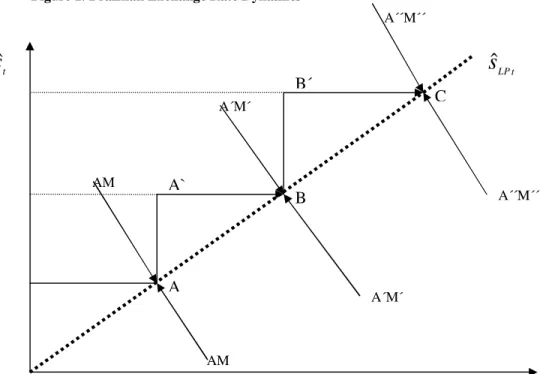
One can represent the exchange rate dynamics of this model (see figure 1) in such a way to draw some insights on the recent Brazilian exchange rate experience. The formal representation of figure 1 suggests the existence of a long term exchange rate, which is not necessarily constant over time.

A to A´, temporarily deviating from the long term equilibrium, but the asset market represented by the AM curve is still at its short run equilibrium. Another equilibrium is taking place when the asset market adjusts to the new exchange rate parity and the short run equilibrium (point B) seems also to be a long term equilibrium point. It is important to consider that what really drives the nominal exchange rate to an overshooting situation and to a new equilibrium is the same mechanism, which is guided by expectations formed in the asset market (AM). Asset market should be understood considering the interactions of financial and monetary markets, or in other words, looking at economic agents allocation choices. The asset market equilibrium is weak and temporary under floating regime, especially under high capital mobility.9 More than a simple equilibrium in the monetary market, as suggested by monetary models of exchange rate determination, here we have a problem of asset allocation and an approximation of the portfolio approach but under high country risk and capital mobility as revealed by the Brazilian experience.

Figure 1. Brazilian Exchange Rate Dynamics

III – Exchange Rate Dynamics in Brazil

The present section of the paper is divided into two parts. One deals with long term issues examining the statistical properties over time for each time series, including the cointegration analysis. The second one focuses on short run issues like volatility and behavior under floating

9 _{The capital account liberalization in Brazil during the 1990s was a process where capital mobility has increased and}

we can consider the economy as facing a scenario of high capital mobility. (see Veríssimo and Holland, 2004). t

s

ˆ

T

t LP

s

ˆ

A

B

C

A`

B´

AM

AM A´M´

A´M´

rates, using statistical instruments and econometric techniques such as variance decomposition analysis, Granger causality tests, among others. What we are really searching for is to answer two important questions. Firstly, did the new floating regime change the mean of the effective exchange rate? And, secondly, what explains the exchange rate volatility?

III.1 – Exchange Rate in Brazil: Long-Term Behavior

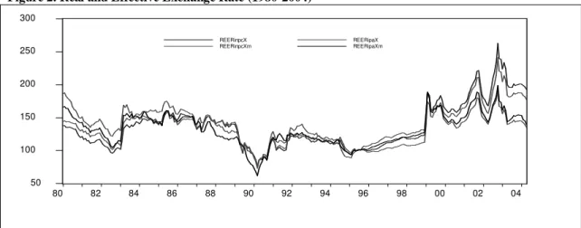
According to figure 2, we can identify two important features of the real effective exchange rate in Brazil, from 1980 to 2004, using monthly data. Firstly, there is an evident change on the mean of the series right after the implementation of the floating regime (beginning of 1999) when deflating the series by the National Consumer Price Index (INPC), where with the Wholesale Price Index (IPA) the series seems to move back towards its 1980s level. Analyzing the period of 1980-1994 as a benchmark in a historical perspective, the exchange rate devaluated more than 50% when using the INPC and only 19% when considering the IPA (table 1). Secondly, there is a strong change in the monthly variance of the exchange rate, from a historical mean of 3.5% (IPA) and 3.99% (INPC)

from 1980 to 199410, to 5.6% (IPA) and 10.8% (INPC) from 1999 to 2004.

On the other hand, analyzing the relationship between exchange rate and wages, according to table 1, we can verify the fact that there is a downward movement from 1980s to 1998 and an upward movement since 1999 that was not able to bring such variables to the same level prior to the Real Plan (1994), and recently it is somewhat around 30% below its historical level.

Most studies on long term exchange rates in Brazil using different samples and methods more frequently than not end up with a conclusion that it is difficult to find empirical evidence supporting the idea that there is a long term equilibrium exchange rate. Therefore, there is no empirical support for the Purchasing Power Parity hypothesis.11 According to Froot and Rogoff (1995), if the real exchange rate is not a stationary process one can suggest that the nominal exchange rate follows domestic and foreign inflation differential, and the Brazilian evidence suggests that the real and effective exchange rate are integrated in order 1, regardless of the deflator used.12

10_{We did not consider the period 1994-1998 as a historical perspective once it was a fixed exchange rate regime.} 11 _{See Kannebly Junior (2003) as an interesting survey and Holland & Valls (1999), where one can see empirical}

evidences to PPP in Brazil.

12 _{Unit root tests, either the Phillips-Perron or the Augmented Dickey-Fuller do not reject the null hypothesis of a unit}

One important question to be asked is if the exchange rate follows a random walk or if it is a

stationary process. Based on the resultsestimated for monthly data, the real effective exchange rate

is not stationary using Phillips-Perron (P-P) Unit Root Tests13. As a preliminary insight we can say

that there is no evidence that changes in nominal exchange rate has followed domestic and foreign inflation differential regardless of the price index used. The real effective exchange rate devaluation has been accompanied by a reversal in the trade balance from a deficit in 1998 (US$6,4 billions) to a surplus in 2003 (more than US$25 billions), which can be considered as an empirical evidence

that changing the exchange rate regime has also implied in changes in the exchange rate level.14

Examining the Brazilian experience, it is easy to observe that there is a strong regime change when looking at the mean and the variance, especially after 1999 when the economy faces the new floating (managed) exchange rate regime. It is important to highlight that the strength of this change depends on the deflator used. There is a clear change in relative prices in favor of the wholesale price index (IPA) and the real effective exchange rate deflated by the IPA is closer to its historical level even when we have the new exchange regime. The same does not happen when we consider the INPC and real effective exchange rate has shifted to a higher (more devaluated) level.

Figure 2. Real and Effective Exchange Rate (1980-2004)

50 100 150 200 250 300

80 82 84 86 88 90 92 94 96 98 00 02 04

REERinpcX

REERinpcXm REERipaXREERipaXm

Source: IPEA (2004)

Notes: REERinpcX = Real and Effective Exchange Rate, using INPC and weighted by total exports;

REERipaX = Real and Effective Exchange Rate, using IPA and weighted by total exports;

REERinpcXm = Real and Effective Exchange Rate, using INPC and weighted by exports of manufactured goods.

13_{Augmented Dickey-Fuller Test was not used because it reveals a tendency to accept the null hypothesis of a unit root}

in time series with structural break.

14_{The empirical results from table 2 (P-P test) suggest that all series in first difference are stationary. To summarize, we}

Figure 3. Variability of Real and Effective Exchange Rate (1980-2004)

-20 -10 0 10 20 30

80 82 84 86 88 90 92 94 96 98 00 02 04

Source: IPEA (2004).

Note: Variability measured by first difference of REERipaX (Real and Effective Exchange Rate, using IPA and

weighted by total exports).

Table 1. Indexes Devaluation of Exchange Rate (1980-2004)

REERinpcX REERipaX REERinpcXm REERipaXm ERw EREw

1980-1994 100 100 100 100 100 100

1999-2004 156 119 142 128 71 70

Notes: REERinpcX = Real and Effective Exchange Rate, using INPC and weighted by total exports;

REERipaX = Real and Effective Exchange Rate, using IPA and weighted by total exports;

REERinpcXm = Real and Effective Exchange Rate, using INPC and weighted by exports of manufactured goods; ERw = Nominal Exchange Rate-Wages; and EREw = Effective Exchange Rate-Wages.

The next step is to pursue an econometric investigation on the dynamics of the exchange rate during the floating regime using daily data, from the 4th _{of January 1999 to the 16}th _{of May 2004. The idea}

is to estimate the equation for the exchange rate as a function of the country risk and domestic and foreign interest rates. Based on the analysis of the time series from figures 4 and 5, one can observe that domestic interest rate (swap360), exchange rate and country risk exhibit long term co-movements, but the same does not apply for the US interest rate (Federal Fund) with respect to the other variables. In order to address this issue in deeper and more rigorous details we developed empirical tests using a VAR (Vector Autoregressive) methodology.

Table 3 - Unit Root Tests for Exchange Rate in level and in first difference Phillips-Perron Test (August 1999 May 2004)

Critical Values Variables Lags Bandwidth* PP Test 1% 5%

ER 3 1 -1.08 -3.44 -2.86

SWAP360 1 5 -2,35 -3.44 -2.86 EMBI+ 4 4 -0.98 -2.57 -1.94 FFUS 2 82 -2.41 3.96 -3.94 DER 0 7 -27.74 -2.57 -1.94 DSWAP360 0 2 -32.8 -3.43 -2.86 DEMBI+ 0 10 -26.07 -2.57 -1.94 DFFUS 0 102 -39.42 -2.57 -1.94 Note: Mackinnon (1996) one-side p-value; Null Hypothesis: If the variable has a unit root.

* Bandwidth: Newey-West using Bartlett Kernel

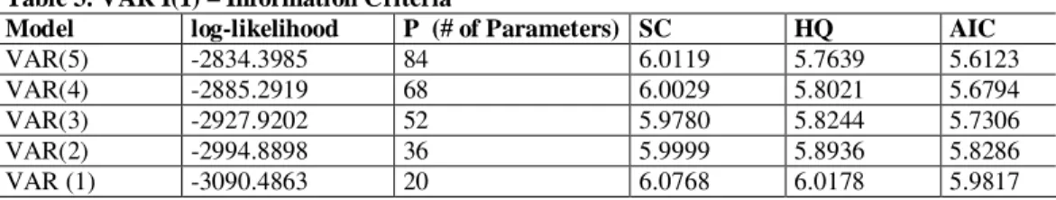
In order to choose the order of each one of our systems we estimate a VAR for four variables (SWAP360, FFUS, ER and EMBI+), including dummy variables when they are significant and necessary to improve our model specification in terms of obtaining better results for Gaussian errors. Table 3 reports the results of the Schwarz (SBC) and Hannan-Quinn (H-Q) tests for system reduction. Whichever lag (order) maximizes the SBC or the H-Q for each country was considered the order of our VAR. The selected system order is 3 according to the Schwarz criteria. Overall, we can say that we have robust results for our models in terms of well-behaved errors, which is well known to be an important result when testing for cointegration.

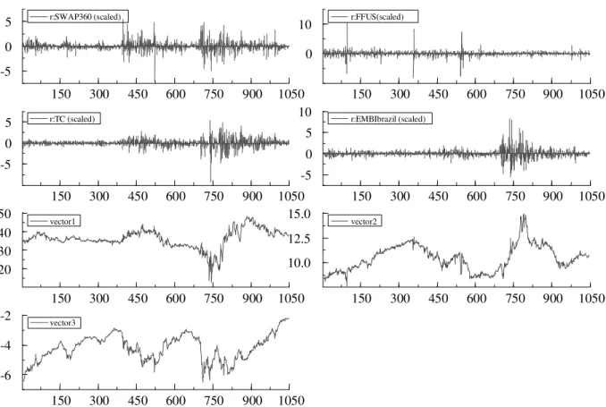
After estimating the VAR, the hypothesis that there are cointegrating vectors in the system was analyzed, following Johansen (1988) and Johansen & Juselius (1990) procedures. The evidence from table 4 suggests that one can not reject the hypothesis that there is one cointegrating vector. For this reason, after testing for vector stationarity, we included an error correction mechanism (ECM) in the exchange rate equation. The Johansen procedure is weak when Gaussian errors are

not accepted and therefore we introduced dummy variables in some VAR specifications.15

Table 3. VAR I(1) – Information Criteria

Model log-likelihood P (# of Parameters) SC HQ AIC

VAR(5) -2834.3985 84 6.0119 5.7639 5.6123 VAR(4) -2885.2919 68 6.0029 5.8021 5.6794 VAR(3) -2927.9202 52 5.9780 5.8244 5.7306 VAR(2) -2994.8898 36 5.9999 5.8936 5.8286 VAR (1) -3090.4863 20 6.0768 6.0178 5.9817

Table 4. Cointegration Statisitics

Rank Trace test [ Prob] Max test [ Prob] Trace test (T-nm) Max test (T-nm)

0 57.38 [0.004]** 36.40 [0.002]** 56.72 [0.005]** 35.98 [0.002]**

1 20.98 [0.370] 13.79 [0.397] 20.73 [0.385] 13.63 [0.410]

2 7.19 [0.563] 6.79 [0.522] 7.10 [0.572] 6.71 [0.532] 3 0.39 [0.531] 0.39 [0.531] 0.39 [0.533] 0.39 [0.533] Notes: ** denotes significance at 1%; T-nm = adjusted for degrees of freedom

Figure 4 – Cointegration Analysis – Residuals and Cointegration Relations

150 300 450 600 750 900 1050 -5

0

5 r:SWAP360 (scaled)

150 300 450 600 750 900 1050 0

10 r:FFUS(scaled)

150 300 450 600 750 900 1050 -5

0

5 r:TC (scaled)

150 300 450 600 750 900 1050 -5

0 5

10 _{r:EMBIbrazil (scaled)}

150 300 450 600 750 900 1050 20

30 40 50

vector1

150 300 450 600 750 900 1050 10.0

12.5 15.0

vector2

150 300 450 600 750 900 1050 -6

-4

-2 _vector3

The next step of our empirical work was to estimate the exchange rate equation as a function of domestic market interest rate (SWAP360), foreign interest rate (FFUS) and country risk (EMBI+). Regressing the first difference of the nominal exchange rate (DER) by OLS (Ordinary Least Square) and using daily data from January 1999 to May 2004 and adding the cointegrating vector, we have the following equation (t-values in parentheses):

The econometric interpretation suggests that changes in the exchange rate are explained by domestic rate and country risk, but there is no evidence that US interest rate plays an important role

to explain movements in the nominal exchange rate for Brazil during the period analyzed.

III.2 –Short-term Exchange Rate Volatility and Interest Rate

There are some important questions to be answered in this section. First, is there any evidence of “excessive” volatility in the Brazilian exchange rate market? Second, has volatility increased since the adoption of the floating regime in 1999?

In general, the exchange rate time series are not stationary, showing conditional autoregressive heteroskedasticity, the errors have no normal distribution, and are asymmetric.16 _{One can suggest}

that the level of exchange rate causes the conditional variance, and based on the Brazilian experience, the variance can change the mean. It is possible to find support for the idea of volatility clustering, that is, periods of high volatility are followed by periods with the same variance magnitude and vice-versa for low volatility and variance. Engle (1982) implemented tests for an ARCH (Autoregressive Conditional Heteroskedasticity) process, encouraged by the evidence that the variance of current residuals could be related to its past level squared or the square of lagged residuals17. Since this pioneer work, a family of conditional heteroskedasticity tests has been developed, like the Generalized ARCH, known as GARCH(p,q). It allows for both autoregressive and moving average components in the heteroskedastic variance18. In this case, the conditional

variance of the errors of the stochastic process

{y

t

}

consists in an ARMA (autoregressive moving

average) process.

According to Bollerslev (1986;1990), a GARGH(p,q) can be defined as:

ht = αo +

i q

=

✫

1

αi

ε

_{t i}2₋ + ✬

= p

1 i

βiht-i

(20)

The stationary condition of a GARCH(p,q), obtained from a Bollerslev (1986), is the following:

16 _{See Engle (1982) in his empirical analysis on mean and variance relationship for British Inflation.}

17 _{The ARCH model is clearly non-linear in terms of the variance, but one can prove that this model is similar to a linear}

process such as ARMA, using squared of variables.

18 _{The GARCH model is estimated by maximum likelihood and there is an assumption that the errors are conditionally}

i q

=

✭

1 αi +

j p

=

✮

1

βj < 1

(21)

When the sum of the

α

i and

β

j parameters is equal to one (1) we have an Integrated GARCH

Model, that is, IGARCH(p, q). Here one can easily obtain a more simplified model such as a GARCH(1,1), when the conditional variance shows the following definition:

ht = αo + α1

ε

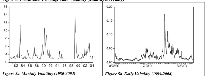
_t2₋₁+ β1ht-1 (22)

The prior section of this paper has shown that there was a significant change in the variance of the exchange rate, considering either the nominal or the real effective concept. According to figures 5a and 5b, we can observe daily and monthly volatility of nominal and real effective exchange rate using a GARCH (1,1) estimation procedure. From a historical perspective, and until the December 1998, taking a look at figure 7a, one can relate the volatility picks with the exchange rate events associated with policymakers’ intervention much more than the changes in market perception of the macroeconomic situation. During this period such events are associated to maxi devaluations and the return of high inflation rates after heterodox stabilization plans have failed during the 1980s and early 1990s. Only after the floating regime in 1999, one can relate high volatility with changes in how the market is evaluating the economy.

Figure 5. Conditional Exchange Rate Volatility (Monthly and Daily) 2 4 6 8 10 12 14 16

82 84 86 88 90 92 94 96 98 00 02 04

Figure 5a. Monthly Volatility (1980-2004)

0.00 0.05 0.10 0.15 0.20

8/23/99 7/23/01 6/23/03

Figure 5b. Daily Volatility (1999-2004)

Figures 6a and 6b illustrate the relationship (or lack of) between domestic interest rate and US interest rate. This phenomenon takes place not because of the insulation properties of the floating regime but due to a specific moment in US monetary policy where interest rates have been extremely low for the past few years. In fact, we have other channels other then foreign interest rates as international shock transmission, such as the country risk and its association to the probability of default and the domestic interest rate19. A closer behavior over time for the exchange rate, country risk and domestic interest rate is illustrated by Figure 7a for the Brazilian economy under floating exchange rates.20

Figure 6. Interest Rate (1999-2004)

Figure 6a. Brazil: Interest Rate Selic and Swap360

0.000 1.000 2.000 3.000 4.000 5.000 6.000 7.000 8.000 8/ 2 0/ 1 99 9 1 0/ 2 0/ 1 99 9 1 2/ 2 0/ 1 99 9 2/ 2 0/ 2 00 0 4/ 2 0/ 2 00 0 6/ 2 0/ 2 00 0 8/ 2 0/ 2 00 0 1 0/ 2 0/ 2 00 0 1 2/ 2 0/ 2 00 0 2/ 2 0/ 2 00 1 4/ 2 0/ 2 00 1 6/ 2 0/ 2 00 1 8/ 2 0/ 2 00 1 1 0/ 2 0/ 2 00 1 1 2/ 2 0/ 2 00 1 2/ 2 0/ 2 00 2 4/ 2 0/ 2 00 2 6/ 2 0/ 2 00 2 8/ 2 0/ 2 00 2 1 0/ 2 0/ 2 00 2 1 2/ 2 0/ 2 00 2 2/ 2 0/ 2 00 3 4/ 2 0/ 2 00 3 6/ 2 0/ 2 00 3 8/ 2 0/ 2 00 3 1 0/ 2 0/ 2 00 3 1 2/ 2 0/ 2 00 3 2/ 2 0/ 2 00 4

Figure 6b. EUA: Effective Federal Fund (FFUS)

Source: Central Bank of Brazil (2004) and CETIP (2004).

19 _{See Holland & Vieira (2003) for the relationship among interest rate, country risk and probability of default in Brazil}

in recent period.

20 _{We are using the SWAP360 rate as domestic interest rate because it is the rate used by the exchange rate market to}

make financial calculus and to take decisions. In the figure 6a one can see the other one, the Over-Selic rate, used in open market and used to the Monetary Authorities to announce the target of the interest rate.

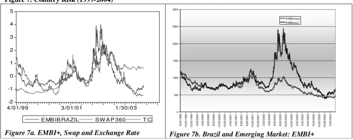
Figure 7. Country Risk (1999-2004) -2 -1 0 1 2 3 4 5

4/01/99 3/01/01 1/30/03 E MB IB RAZIL SW A P 360 T C

Figure 7a. EMBI+, Swap and Exchange Rate

0 500 1000 1500 2000 2500 3000 8/ 20 /1 99 9 10 /2 0/ 19 99 12 /2 0/ 19 99 2/ 20 /2 00 0 4/ 20 /2 00 0 6/ 20 /2 00 0 8/ 20 /2 00 0 10 /2 0/ 20 00 12 /2 0/ 20 00 2/ 20 /2 00 1 4/ 20 /2 00 1 6/ 20 /2 00 1 8/ 20 /2 00 1 10 /2 0/ 20 01 12 /2 0/ 20 01 2/ 20 /2 00 2 4/ 20 /2 00 2 6/ 20 /2 00 2 8/ 20 /2 00 2 10 /2 0/ 20 02 12 /2 0/ 20 02 2/ 20 /2 00 3 4/ 20 /2 00 3 6/ 20 /2 00 3 8/ 20 /2 00 3 10 /2 0/ 20 03 12 /2 0/ 20 03 2/ 20 /2 00 4 EMBIemerg EMBIbrazil

Figure 7b. Brazil and Emerging Market: EMBI+ Source: Central Bank of Brazil (2004), CETIP(2004) and J.P.Morgan(2004).

Table 5 describes some basic statistics for five time series (country risk, exchange rate, market interest rate, government interest rate, and foreign interest rate). At first glance we can say that the exchange rate changes less than the country risk but it is closer to the domestic (market) interest rate. It is worth noting that the exchange rate assumed values ranging from 1.72 to 3.95 real per dollar in a relatively short period of time. At the same time, the country risk, measured by the J.P.Morgan EMBI+ has shifted from 410 to 2436 points, and the interest rate (SWAP360) changed from an annual rate of 14.98% to 32.69%. Setting aside the numbers and looking at the general picture, it is fair to saw that the floating regime in Brazil relies on a weak combination of significant variability and vulnerabilities, where its implementation has not been followed by periods where other external financial variables are more accommodative, besides the trade

balance, according to figure 8.21 One can see a strong co-movement between trade balance and

real and effective exchange rate since the floating regime in 1999. We used the Hodrick-Prescott filter as a smoothing method that is widely used among macroeconomists to obtain a smooth estimate of the long-term trend component of a series22_.

21 _{It should be reminded that since 2001 the Brazilian exchange rate have played an important role in improving the}

trade balance when it started to show surplus outcomes. 22

Hodrick and Prescott to analyze postwar U.S. business cycles used this method for the first time. Technically, the Hodrick-Prescott (HP) filter is a two-sided linear filter that computes the smoothed series (s) of (y) by minimizing the variance of (y) around (s), subject to a penalty that constrains the second difference of (s). In other words, the HP filter chooses to minimize:

(

)

2

1 T

2

t t 1 t t t1

2 t T 1 t t ) s s ( ) s s ( ) s y ( ✾ ✾ − = + − = − − − λ +

− The penalty parameter controls the smoothness of the series

Table 5. Basic Statistics – Daily Data (1999-2004) EMBI+

(points)

ER (R$/US$)

SWAP360 (annual %)

SELIC (annual %)

FFUS (annual %)

Mean 921 2.51 21.65 19.07 3.32

Median 800 2.46 20.97 18.69 2.03

Maximum 2436 3.95 32.69 26.32 7.03

Minimum 410 1.72 14.98 14.99 0.86

Standard Deviation 378 0.58 4.35 3.03 2.15

Variation Coefficient 41 23 20 16 66

Notes: EMBI+ = JPMorgan Country Risk; ER = Nominal Exchange Rate: SWAP 360 = Brazilian Interest Rate in

Swap Market to 360 days; SELIC = Brazilian Interest Rate in Open Market; FFUS = US Effective Federal Fund.

Figure 8. Brazil: Trade balance and Real and Effective Exchange Rate – Hodrick-Prescott (HP) filter (1980:01-2004:04)

-1000 0 1000 2000 3000

100 120 140 160 180

80 82 84 86 88 90 92 94 96 98 00 02 04

TBhp REERhp

Source: Central Bank of Brazil (2004) and IPEA (2004).

Note: TBhp = Trade Balance smoothed by HP filter; REERhp = Real and Effective Exchange Rate

using IPA and weighted by total exports and smoothed by HP filter.

The Granger causality tests reported on table 7 for two lags and using all variables in first difference suggest the existence of bi-causality for domestic interest rate (swap360) and exchange rate, and for country risk (EMBI+) and exchange rate, and the results are robust to changes in the number of lags. There is no causality (Granger) for foreign interest rate (Federal Funds) and exchange rate, and for foreign and domestic (swap360) interest rates.23 Other than this, causality was found from country risk to domestic interest rate for any lags used, but the other way round indicates mixed evidence for causality since it can be found for five, four (only at 10%), three and two lags, but no causality for one lag. Finally, there is no causality for country risk (EMBI+) and foreign interest rates (Federal Funds) for any number of lags.

23 _{One possible explanation for this result can be associated to the fact that U.S. monetary policy assumed a specific}

Table 6. VAR I(0) – Information Criteria

Model log-likelihood P (# of Parameters) SC HQ AIC

VAR (5) -2851.1577 84 _{6.0441 5.7961 5.6445} VAR (4) -2853.6774 68 _{5.9421 5.7413 5.6186} VAR (3) -2908.3030 52 _{5.9402 5.7867 5.6929} VAR (2) -2956.6094 36 _{5.9263 5.8200 5.7550} VAR (1) -3028.2187 20 _{5.9571 5.8980 5.8620}

Table 7. Granger Causality Test Sample: 4/01/1999 4/16/2004 Lags: 2

Null Hypothesis: Obs F-Statistic Probability

DFFUS does not Granger Cause DEMBI 1164 0.41218 0.66230 DEMBI does not Granger Cause DFFUS 0.24650 0.78158 DSWAP does not Granger Cause DEMBI *** 1168 4.83920 0.00807 DEMBI does not Granger Cause DSWAP *** 17.5823 3.0E-08 DTC does not Granger Cause DEMBI *** 1168 5.78699 0.00316 DEMBI does not Granger Cause DTC *** 41.1974 0.00000 DSWAP does not Granger Cause DFFUS 1164 1.11018 0.32985 DFFUS does not Granger Cause DSWAP 0.16884 0.84467 DTC does not Granger Cause DFFUS 1164 1.20675 0.29954 DFFUS does not Granger Cause DTC 0.25273 0.77672 DTC does not Granger Cause DSWAP 1168 1.04864 0.35074 DSWAP does not Granger Cause DTC *** 17.0352 5.1E-08 *, ** and *** denotes significance level at 10%, 5% and 1% respectively

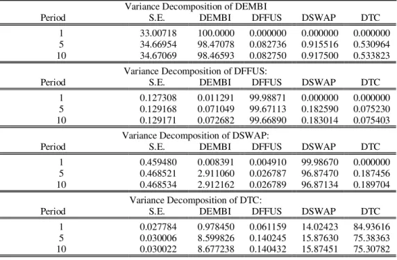
Table 8 - Variance Decomposition

Variance Decomposition of DEMBI

Period S.E. DEMBI DFFUS DSWAP DTC 1 33.00718 100.0000 0.000000 0.000000 0.000000 5 34.66954 98.47078 0.082736 0.915516 0.530964 10 34.67069 98.46593 0.082750 0.917500 0.533823

Variance Decomposition of DFFUS:

Period S.E. DEMBI DFFUS DSWAP DTC 1 0.127308 0.011291 99.98871 0.000000 0.000000 5 0.129168 0.071049 99.67113 0.182590 0.075230 10 0.129171 0.072682 99.66890 0.183014 0.075403

Variance Decomposition of DSWAP:

Period S.E. DEMBI DFFUS DSWAP DTC 1 0.459480 0.008391 0.004910 99.98670 0.000000 5 0.468521 2.911060 0.026787 96.87470 0.187456 10 0.468534 2.912162 0.026789 96.87134 0.189704

Variance Decomposition of DTC:

The variance decomposition results reported in table 8 show that changes in the exchange rate, domestic and foreign interest rates do not play an important role in explaining movements in the country risk, and the same interpretation is valid for changes in foreign interest rates that can be poorly explained by changes in the domestic interest rate, nominal exchange rate and country risk. On the other hand there are two interesting results. First, the variance decomposition of the domestic market interest rate (swap360) is partially explained by the changes in country risk (around 3%), where the variance of the exchange rate seems to be conditioned to the changes in the country risk (8.67%) and in the domestic interest rate (15.87%).

IV - EXCHANGE RATE AND FOREIGN LIQUIDITY

We can now analyze the relationship between floating regime and international exchange reserves. It is known that, under more rigid exchange rate regimes, foreign exchange reserves should be at a level high enough to deal with possible trade or current account deficits. A significant fall on international reserves is generally associated with episodes of foreign exchange crises and in this situation one can expect a higher probability that countries with more rigid exchange regimes will move to a new and more flexible regime.

"dirtiness" for emerging economies when compared with advanced countries. This can be explained due to a higher dependence on foreign capital flows and frequent liquidity restrictions and sudden credit squeezes, and because nominal price volatility of tradable goods may have a positive impact on inflation volatility.

Initially, it can be questioned whether or not movements in foreign exchange reserves on a floating regime works as if it is an accommodative tool. A preliminary graphic analysis (figure 8a) seems to indicate that there has been a strong upward movement in foreign exchange reserves during most of the decade, especially in period of quiescence, but a strong downward movement in situations of stress usually associated with both external (Asia 1997 and Russia 1998) and domestic (Brazil -1999) episodes.

Figure 8. International Liquidity Indicators

Figure 9a. International Reserves / Imports Monthly Data (1990-2004)

Figure 9b.External Debt / Exports and Adjusted International Liquidity / Imports – Annual Data (1997-2003)

Source: Central Bank of Brazil (2004).

Concluding Remarks

The literature on floating exchange rate regimes can be considered somehow skeptical since controversies and different empirical outcomes seems to be the rule rather than the exception. Floating regimes for developing countries have distinct features since the pass-through from devaluation to inflation is a frequent concern and free floating has almost never been adopted in these countries where international reserves are still an important variable do manage the exchange rate in a world where financial crisis are quite frequent.

The empirical analysis of the Brazilian experience under floating rates has provided some useful insights. One of them is that the exchange rate does not seem to be driven by foreign interest rates, which could be considered an advantage in terms of setting apart the behavior of the exchange rate and possible external shocks. On the other hand, domestic market interest rate (swap360) and country risk (EMBI+) play an important role on the exchange rate dynamics during the floating period in Brazil. Other than this the empirical results suggest not only a country risk endogeneity to domestic interest rate but also the exchange rate seems to display a certain degree of endogeneity. This can be considered as unexpected empirical evidence since the Brazilian economy did not take advantage of a favorable scenario of lower US interest rates and it was necessary to maintain high real interest rates to prevent undesirable inflation impacts from exchange rate movements (pass through). This phenomenon is clear when we take into account the emphatic co-movement among the country risk (or the probability of default), the interest rate and the exchange rate.

-5,00 10,00 15,00 20,00 25,00 jan/9 0 jul/9 0 jan/9 1 jul/9 1 jan/9 2 jul/9 2 jan/9 3 jul/9 3 jan/9 4 jul/9 4 jan/9 5 jul/9 5 jan/9 6 jul/9 6 jan/9 7 jul/9 7 jan/9 8 jul/9 8 jan/9 9 jul/9 9 jan/0 0 jul/0 0 jan/0 1 jul/0 1 jan/0 2 jul/0 2 jan/0 3 jul/0 3 jan/0 4 0 1 2 3 4 5 6

After the theoretical and empirical analysis pursued in this paper regarding the exchange rate in Brazil under floating rates we can say that there are specificities that should be taken into account in order to understand its dynamics in more detail. One of these is the straight link among of interest rates, exchange rate and the degree of indebtedness under a macroeconomic situation where economic policy is guided by managing the exchange rate and inflation targeting.

Bibliography

Alesina, A. & Wagner, A. (2003). Choosing (and Reneging On) Exchange Rate Regimes. NBER

Working Paper Series, 9809, June, 2003.

Bollerslev (1986). Generalized Autoregressive Conditional Heteroskedasticity. Journal of

Econometrics, 31.

Bollerslev (1990). Modelling the Coherence in Short-run Nominal Exchange Rates: a Multivariate

Generalized ARCH Approach. Review of Economics and Statistics. 72.

Calvo, G. A. e Mishkin, F. S. (2003) The Mirage of Exchange Rate Regimes for Emerging Market

Countries. NBER Working Paper, 9808, Junho, 2003.

Calvo, G. & Reinhart, C. (2002) Fear of Floating. Quarterly Journal of Economics, May, 2002. .

Calvo, G. (2000). The case for hard pegs in the brave new world of global finance. ABCDE Europe,

Paris, June 26, (draft).

Central Bank of Brazil (2004). Times Series. Brasília: DF. http://www.bcb.gov.br

CETIP (2004). Time Series. São Paulo, Brazil. http://www.cetip.com.br

Dornbusch, R (1976). Expectations and Exchange Rate Dynamics. Journal of Political Economy,

December, 1976.

Engle, R (1982). Autoregressive Conditional Heteroskedasticity With Estimates of the Variance of U.K. Inflation. Econometrica 50 (1982).

Edwards, S. & Levy-Yeyati, E. (2003) Flexible Exchange Rates as Shock Absorbers. NBER

Working Paper Series, 9867, June, 2003.

Fischer, S. (2001). Exchange Rate Regimes: Is the Bipolar View Correct? American Economic

Review, May 2001.

Frankel, J. (1999). No Single Currency Regime is Right for All Countries or at All Times. NBER Working Paper Series, 7338, September, 1999.

Frankel, J. (2003) Experience of and Lessons from Exchange Rate Regimes in Emerging

Froot, K. & Rogoff, K. Perspectives on PPP and Long-Run Real Exchange Rates. Grossman G. and

K. Rogoff (eds.) Handbook of International Economics, Vol. III., Chapter 32, North Holland,

1995.

Ghosh, A. R; Gulde, A.M.; and Wolf, H.C. (2002) Exchange Rate Regimes: Choices and

Consequences. MIT Press, 2002.

Goldfajn, I. & Olivares, G. (2001) Can Flexible Exchange Rate Still `Work` in Financially Open

Economies? G24 Discussion Paper Series, UNCTAD, January, 2001.

Hausmann, R.; Panizza, U.; and Stein, E. (2000) Why Do Countries Float the Way they Float?

Inter-American Development Bank Working Paper, 418, Research Department, May, 2000.

Holland, M. & Valls, P. (1999). Taxa Real de Câmbio e Paridade de Poder de Compra no Brasil.

Revista Brasileira de Economia. 53(03). Rio de Janeiro: Fundação Getúlio Vargas.

Holland, M. & Vieira, F. (2003). Country Risk Endogeneity, Capital Flows and Capital Controls in Brazil. Revista de Economia Política, Vol. 23(1), Jan-Mar, 2003.

IPEA (2004). Ipeadata. Brasília: DF. http://www.ipea.gov.br

Johansen, S (1988). Statistical Analysis of Cointegrating Vectors. Journal of Economic Dynamics

and Control, 12.

Johansen, S. & Juselius, K. (1990). "Maximum Likelihood Estimation and Inference on Cointegration". Oxford Bulletin of Economics and Statistics, 52.

J.P.Morgan. Research. New York: US. http://www.jpmorgan.com

Kannebly Junior, S (2003). Paridade de Poder de Compra no Brasil – 19681 1994. Estudos

Econômicos, 33(4). São Paulo: IPE/USP.

Larrain, F. & Velasco, A. (2001) Exchange Rate Policy in Emerging Markets: The Case for

Floating. Working Paper, Harvard University, April, 2001.

Levy-Yeyati, E. & Sturzenegger, F. (2001) To Float or to Trail: Evidence on the Impact of

Exchange Rate Regimes. Working Paper, Universidad Torcuato Di Tella, January, 2001.

MacKinnon (1991). Critical Values for Cointegration Tests. R. F. Engle & C. W. Granger.

Long-run economics relationships. Oxford. University Press, 1991.

Mishkin, F. & Savastano (2000). Monetary Policy Strategies for Latin America. NBER Working

Paper 7617, March 2000.

Reinhart, C.M. & Reinhart, V.R. (2003) Twin Fallacies About Exchange Rate Policy in Emerging

Markets. NBER Working Paper Series, 9670, April, 2003.

Reinhart, C. M. & Rogoff, K.S. (2002) A Modern History of Exchange Rate Arrangements: A

Reinhart, C. M.; Rogoff, K.S.; and Savastano, M.A . (2003) Addicted to Dollars. NBER Working

Paper Series, 10015, October, 2003.

Rogoff, K.S.; Husain, A . M.; Mody, A.; Brooks, R.; and Oomes, N. (2003) Evolution and

Performance of Exchange Rate Regimes. IMF Working Paper, 243, Research Department,

December, 2003.

Velasco, A. (2000) Exchange-rate Policies for Developing Countries: What Have We Learned?

What Do We Still Not Know? UNCTAD, G-24 Discussion Paper Series, No.5, June, 2000.

Veríssimo, M. & Holland, M (2004). Liberalização da Conta de Capital e Fluxos de Portfólio para o