ABSTRACT: This study aimed to analyze the time series behavior of the Southern Oscillation Index through techniques using Fast Fourier Transform, computing the autocorrelation function, and the calculation of the Hurst coeficient. The methodology of Hurst Exponent calculation uses different lags, which are computed in the time series of Southern Oscillation Index. The persistent behavior in the time series can be characterized by calculating the Hurst Exponent, seeking for more behavioral information, as the existence of persistence and/or terms of long-range memory in the series. The results show a persistence of the climate in terms of long-memory Southern Oscillation Index time series, which can help to understand a complex dynamic behavior in climate effects at global-scale level and speciically its inluence in northeastern Brazil, in the region of the Alcântara Launch Center. The R package tseriesChaos was used in the analysis of the Southern Oscillation Index time series, estimating the largest Lyapunov exponent, which indicates the existence of chaotic behavior in time series. The resampling technique was used in a permutation test between the surface wind data in the São Luís airport, Maranhão State, and the Southern Oscillation Index. The permutation test results showed that the time series of monthly average wind speed in the São Luís airport is correlated with the variability of Southern Oscillation Index, statistically correlated to the conidence interval at the 5% level. The results showed the possibility of using autoregressive models to represent average variable meteorology in the behavior analysis as well as trends in the climate, more speciically a possible climatic inluence of El Niño-Southern Oscillation in wind strength in the Alcântara Launch Center.
KEYWORDS: Time-series analysis, Hurst Exponent, Permutation test.
The Long-Range Memory and the Fractal
Dimension: a Case Study for Alcântara
Cleber Souza Corrêa1, Daniel Andrade Schuch2, Antonio Paulo de Queiroz1, Gilberto Fisch1, Felipe do
Nascimento Corrêa1, Mariane Mendes Coutinho1
INTRODUCTION
Sea surface temperature conditions in the tropical Paciic are important drivers of the atmospheric circulation and can have a major inluence on the global climate. he El Niño-Southern Oscillation (ENSO) is a key component of the climate system (Capotondi 2013) and it is important to understand possible changes in its variability, which may be due to natural processes, such as the decadal variability of climate or anthropogenic efects. he dynamic behavior of ENSO is very complex, and it is diicult to predict its time series variations. he Southern Oscillation Index (SOI) time series signal is composed of a set of geophysical forcing with diferent temporal scales, some of long time as the cycles of solar activity and/or the interaction atmosphere-ocean, involving a planetary scale. he Southern Oscillation is a seesaw in surface air pressure between the tropical eastern and the western waters of the Paciic Ocean. SOI is calculated as the standardized anomaly of the surface air pressure diference between Tahiti, in the Paciic Ocean, and Darwin, Australia, in the Indian Ocean.
The Southern Oscillation is a dynamic coupled ocean/ atmosphere process that influences the planetary scale. It characterizes certain phases: when the situation is positive, it means that there are higher pressure values in Tahiti and lower ones in Darwin (La Niña); the negative phase is when the pressure values are lower in Tahiti and higher in Darwin (El Niño); and in the neutral phase there are no signiicant values. ENSO is a planetary-scale phenomenon that occurs naturally in the tropical Paciic with global and highly-relevant impacts, afecting greatly the human society. El Niño refers to the heating
1.Departamento de Ciência e Tecnologia Aeroespacial – Instituto de Aeronáutica e Espaço – Divisão de Ciências Atmosféricas – São José dos Campos/SP – Brazil.
2.Departamento de Ciência e Tecnologia Aeroespacial – Instituto Tecnológico de Aeronáutica – Programa de Pós-Graduação em Ciências e Tecnologias Espaciais – São José dos Campos/SP – Brazil.
Author for correspondence: Cleber Souza Corrêa | Departamento de Ciência e Tecnologia Aeroespacial – Instituto de Aeronáutica e Espaço – Divisão de Ciências Atmosféricas | Praça Marechal Eduardo Gomes, 50 – Vila das Acácias | CEP: 12.228-904 – São José dos Campos/SP – Brazil | Email: [email protected]
above normal in the tropical Paciic Ocean, which occurs with a frequency of 2 –7 years. Its opposite phase, when the tropical Paciic Ocean is colder than normal, is known as La Niña. hese sea surface temperature changes afect the weather with values above or below the climatological ones.
Capotondi et al. (2015) improved the determination and understanding of ENSO, its predictability and the existence of teleconnections. However, given the complexity and impacts of ENSO, a better analysis of the spatial patterns and their evolution is required. Newman (2007) concludes that the long-term predictability exists; however, due to complex characteristics of the dynamic system in the planetary circulation, the canonical ENSO and the Paciic Decadal Oscillation (PDO) patterns, the inluence of the interaction of these systems creates a complex structure, which consists of 2 stationary eigenmodes that are weaklier damped. hese eigenmodes can represent diferent efects: the canonical ENSO (Barnston and Ropelewski 1992; Gershunov and Barnett 1998; Takahashi et al. 2011) between the years 1900 – 2002 may represent the inluence of anthropogenic nature and multidecadal fluctuations of a pattern that is potentially a natural decadal variability. he predictability of these stationary eigenmodes is signiicantly increased by the coupling of these eigenmodes between the North Paciic region and its tropical oceanic part.
Gershunov and Barnett (1998) showed that the PDO has a modulatory efect on climatic patterns creating ENSO events. As a result, there are important characteristics to be observed: when the phase is El Niño, that stage is likely to be more intense when the PDO is highly positive; on the other hand, the La Niña phase is more intense when the PDO is strongly negative. his behavior does not mean that the PDO physically controls the dynamic ENSO, but the resulting climatic patterns show the interaction between them.
he inluence of the Southern Oscillation in the northeastern Brazil climate has already been well-studied in the literature (e.g. Enield and Mayer 1997; Uvo et al. 1998; Andreoli and Kayano 2006; Gonzalez et al. 2013). It is known that negative anomalies of SOI (El Niño) are associated with decreasing rainfall in northeastern Brazil.he study of SOI time series can provide guidance to understand the associatedin the atmospheric ity of theiated ocean/atmosphere coupling dynamics in the Paciic Ocean and its inluence on the Walker and Hadley circulations. Changes in position and intensity of the Hadley and Walker cells are associated with changes in the large-scale atmospheric circulation patterns, which directly afects the meteorological
conditions over the northeastern region of Brazil. his study aimed to interpret possible stationary signals, associated with a repetitive behavior in terms of long-range memory in SOI time series, as well as their inluence on temporal variability of climate conditions in northeastern Brazil — Alcântara Launch Center (ALC).
METHODOLOGY
SOUTHERN OSCILLATION INDEX DATA
SOI data were obtained from the web page of the National Weather Service - Climate Prediction Center (www.cpc.ncep.noaa. gov/data/indices/). Monthly data normalized in the 1951 –2015 period were used. The AutoSignal© software version 1.6 for Windows was employed to compute the autocorrelation function, which was calculated using the Fast Fourier Transform (FFT; Temperton 1985). he same sotware was used to estimate the Hurst Exponent (H) and generate graphs for analysis.
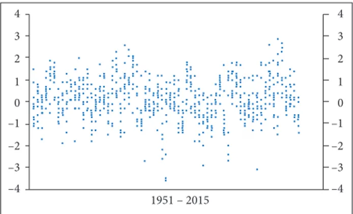
Figure 1 shows SOI time series analyzed to calculate H, using the rescaled range (R/S) analysis. H is used to represent the behavior of time series, which presents persistence of features associated with a memory efect.
Figure 1. SOI from January 1951 to August 2015.
4
3
2
1
0 –1
–2
–3 –4
1951 – 2015
4
3
2
1
0 –1
–2
–3 –4
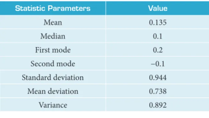
Table 1 presents statistical values of SOI time series. he raw data of this series were treated in Microsot® Excel, in which the
HURST EXPONENT —
R
/
S
METHOD
For a sequence (Xt)n
t=1 of a time series, consider a
partial sum Yk = ∑k
t=1 Xt— 1≤ k ≤ n and a sample variance
S2
n = (n – 1) –1 ∑n
t=1 (Xt – Xn)
2, where X n = n
–1 ∑n
t=1 Xt is a sample
mean. Rescaled adjusted range statistic R/S introduced by Hurst (1951) is deined as:
distribution with a mean equal to 0, the signal is set to be Gaussian white noise.
A normally-distributed or Gaussian sequence may have a cumulative white noise and is known as regular Brownian motion or random walk (Kac 1947; van Horne and Parker 1967). he range or distance covering a variable in the normal Brownian motion will increase in proportion to the square root of time. To calculate the growth that may exist in a time series, a type of time-scaling ratio is used by the partitioning elements (number of observations) and generates an average of the other groups. he use of R/S analysis allows to obtain the statistic of fractal noise process and ofers it as an alternative to the traditional Gaussian normal distribution.
he H variability of behavior can be assigned as the value calculated by the physical behavior of the analyzed time series; an H value equal to 0.5 would indicate no long-term memory. Higher H values indicate a growing presence of such an efect in the series. he duration of this memory efect is oten visible as persistent and can be cyclic or not. An H value of 0.5, which features in its accumulated data series, is a random walk or pure Brownian motion. he dataset analyzed consists of true white noise in which each observation is completely independent of all previous observations, and the estimated autocorrelation series is essentially 0 everywhere, except at the 0 lag. Since
H is less than 0.5, the temporal series have an anti-persistent behavior. Each value in the series tends to be more likely to have a negative correlation with the previous values.
hese data series revert the signals more oten than would be true for the white noise. Such systems are rare in geophysical time series. Much more common in nature are time series that present estimates of H values above 0.5. hese characteristics in the behavior of the series, which are persistent, contain a memory efect. herefore, each value of the series may be associated with a number of previous values of the same series. he modeling of autoregressive processes depends on exactly this purpose. For a persistent series, the series with autocorrelation tend to decrease their autocorrelation to 0. Both the analysis by estimating H and the correlation mapping show the memory efect on time series under review.
he hurstexp (x) function of the R package PRACMA version 3.2.2 (2015), from the R Foundation for Statistical Computing, calculates H. his relationship was derived from the MATLAB®
code of Weron (2002), published in the MATLAB® central.
his function returns a list of diferent deinitions of H with diferent adjustments in their calculations, which are deined
Statistic Parameters Value
Mean 0.135
Median 0.1
First mode 0.2
Second mode −0.1
Standard deviation 0.944
Mean deviation 0.738
Variance 0.892
Table 1. Statistical data of SOI series, with n = 775 values.
(1)
Observe that the numerator Range (R) in Eq. 1 can be viewed as a range of partial sums of Xt – Xn — t = 1, …, n — or, equivalenttly, as the sum of the maximal and minimal distance of the partial sums Yk — k = 1, …, n — from a line passing through Y0= 0 and Yn. he range (R) should be divided by the standard deviation (S) of the elements of time series to produce a standardized sequence R/S or resized value range. hus, R/S
is a measure of lutuations of the parcial sums of (Xt)n t=1 scaled
by the standard deviation of observations.
with the following components: Hs — simpliied approach R/S;
Hrs— simpliied approach corrected H; He — empirical H;
Hal— corrected empirical H; and Ht —theoretical H. hese diferent approaches are estimates of the H method, the corrected
R/S method and the corrected empirical method. he results are sometimes very diferent, depending on the series analysis in the study, which can be interpreted as estimates with highly-questionable values.
FRACTAL DIMENSION
he random walks can be readily generalized to characterize fractal processes (Mandelbrot 1977, 1982) by introducing an additional parameter: H (0 < H < 1). he variance is proportional to Δt2H. In a fractal process, successive increments are correlated
with coeicient of correlation ρ, independently of the time step h, where ρis deined by the formula, using the moment technique of order 2 (Hastings and Sugihara 1993):
the largest Lyapunov exponent of a given scalar time series using the algorithm of Kantz (Hegger et al. 1999) and function lyap computes the Lyapunov regression coeicients for the time series segment given as input, in this case, SOI data. Tools to evaluate the maximal Lyapunov exponent of a dynamic system from a univariate time series provide a parameter that characterizes the dynamics of an attractor. It measures the rate of divergence of neighboring orbits within the attractor and thus quantiies the dependence or system sensitivity to initial conditions. he existence of at least 1 positive Lyapunov exponent is a strong indication of the presence of chaos in the system.
PERMUTATION TEST
he permutation test is used to analyze the relationship between the signals in the temporal series of SOI and the monthly means of surface wind and monthly means of maximum surface wind, from January 1951 to December 1999 (Good 2005; Collingridge 2013). he wind data used were from the São Luís Airport near the ALC. By deinition, the vector P is the wind monthly mean and J (N × 1) is the monthly value of SOI. he test seeks to make random permutations of J, keeping P ixed. For each permutation, the correlation between vectors P and
J was calculated, resampling the series in the order of 10,000 times, thus building the distribution of correlations (r). From these distributions, the value that represents the conidence interval at the 5% level of the correlations in the upper or lower tail of distributions (r critical) can be obtained. he critical value of the correlation at 10,000 times is permuted, ordered from the smallest to the largest value; the calculated value at the 9,500º position is the critical one at the 5% level in the reconstructed distribution (in the upper tail) or in the lower tail; the critical value is that in the 500º position. he time series contains 587 monthly values of wind average speed and maximum wind average values. he permutation test method is statistically more robust than the classical one to test the correlation signal between diferent series that have low correlation values.
RESULTS
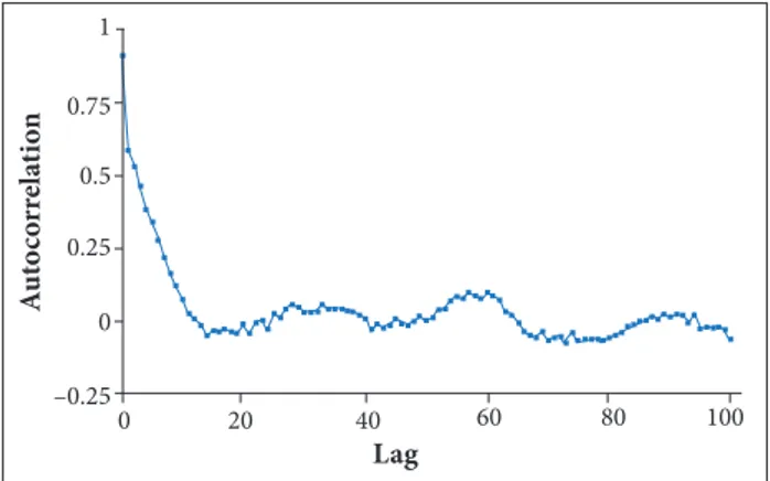
Figure 2 shows the behavior of the autocorrelation function, in which the time series decays to 0 for a 13-month period (lag 13). he autocorrelation function exhibits positive correlation
(2)
where: ρ= 0; H = 0.5, which is a random process.
Mandelbrot (1983) and Goldberger (1996) created a deinition of fractal dimension: it is an index that seeks to characterize patterns, whose order is fractal sets or the quantiication of that nature in its complexity as a reason applied to change his own scale. he fractal dimension can be measured in 2 diferent ways; one of which is geometrically and the other is carried out by probability space. More useful to signal analysis is the deinition of fractal dimension that uses probability space 1/H. By this deinition, a time series with a memory efect will have a fractal dimension between 1.0 and 2.0.
LYAPUNOV EXPONENT
Table 2. Results of the function hurstexp (x) from R package.
Hurst exponent Value
Simple R/S Hurst estimation 0.694
Corrected R over S Hurst exponent 0.775
Empirical H 0.762
Corrected empirical H 0.739
heoretical H 0.533
of about 0.14 for the return times (persistence characteristics) between 25 and 40 lag (2 –3 years) and between 52 and 64 lag (5 – 6 years), with higher signiicance for the latter. In the analysis of autocorrelation function in a time series, with a magnitude of the order of 0.14, this value should not be interpreted as a simple randomness in the time series but as a value of relative signiicance. It may represent possible temporal scale inluences with periods of 2 – 3 and 5 – 6 years, respectively. he results were similar to those obtained by An and Wang (2000) using another method: wavelet analysis. hey showed that the period of oscillation has increased from 2 – 4 years (high frequency), in 1962 – 1975, to 4 – 6 years (low frequency), in 1980 – 1993.
or highly-periodic behavior. The results for H calculation were: H = 0.561; S = 0.013; fractal dimension 1/H = 1.78 and coefficient of determination R2 = 1 − (SSE/SSM) = 0.911,
where SSE is the sum of squared errors (residuals) and SSM is the sum of squares around the mean; weighted H = 0.704; weighted S = 0.007; weighted fractal dimension 1/H = 1.420 and R2, weighted by S, was: R2 = 1 − (SSE/SSM) = 0.998. he
coeicient of correlation ρ= 0.088, in the time series, has a fractal correlation value of about 10%, and the coeicient of correlation weighted by S is 0.326.
Figure 3. H of SOI time series calculation between 1951 and 2015, normalized by S.
Figure 2. Series of autocorrelation of SOI values between 1951 and 2015.
1
0.75
0.5
0.25
–0.25
0 20 40 60 80 100
L a g
A
u
to
co
rr
el
at
io
n
0
H urst Exponent
R
/
S
n obs 100
100 1,000
10
10 1
1
Jin et al. (1996), analyzing ENSO and the existence of annual and sub-harmonic cycles of frequency block and aperiodicity, observed the transition and the occurrence of chaotic regimes close to 4 years and with a quasi-biennial peak, being produced by a dynamic of non-linear interactions.
In the study of Chang et al. (1995), on the interactions between the seasonal cycle and ENSO in an intermediate coupled Ocean-Atmosphere model, the ENSO cycle falls within a sandwiched regime between 3- and 2-year frequency-locking regimes. When the existence of a strange attractor for SOI with a fractal dimension of 2.5 to 6 (with a value close to 5.2) had been estimated, the analysis was performed by a simulation of 1,000 years using the values of monthly SST time series. he observations in their study suggest a change of frequency, and this was accompanied by a signiicant change in the structure of coupled ENSO mode. his result shows the trend of persistency in decadal time series.
Figure 3 shows the statistic range and suggests a positive long-range autocorrelation. he distribuition shows persistent
SOI time series with the H calculation presents a long-range memory with persistence, with values of H = 0.561 and 1/H of about 1.78 with fractal dimension. hese results can be interpreted as the relative tendency of a time series to strongly regress to its mean or to be grouped in 1 direction (Kleinow 2002). he results in Table 2 show that the H estimates using the function hurstexp (x) in R produce values above 0.5, characterizing a time series with long-range memory.
(1995), who propose that the ENSO irregularity can be viewed as a chaotic low-order process driven by the seasonal cycle. he main characteristic of the behavior of chaotic systems is a high sensitivity in the initial conditions, which implies that the evolution of the system can be modiied by small disturbances in the system.
In the years of El Niño occurrence (negative SOI), the characteristics of dynamic systems in the equatorial region (the Hadley and Walker circulations) presented signiicant alterations, and their efects inluence atmospheric behavior in the Brazilian northeast. Operationally, this would inluence directly the ALC, with greater intensity to the wind proile near the surface.
Marques and Oyama (2015) conducted a study on the interannual variability of precipitation in ENSO-neutral years for the ALC. Using various gridded datasets for the 1951 – 2010 period, the authors observed that, below average precipitation, it was related to strong east-norteasterly low-level winds (925 hPa) and northward of the interhemispheric gradient of the sea surface temperature anomalies over Atlantic (GRAD), as well as that, for El Niño conditions, northward GRAD would intensify the negative precipitation anomalies in the northern-northeastern Brazil.
Figure 6 presents, in a similar manner, the test shown in Fig. 4, but the results show the correlation between SOI series and the monthly average of the wind maximums. he results statistically showed a correlation between the signals of the time series with a signiicant conidence interval at the 5% level. he averages of the monthly maximum winds would be higher in months with negative SOI (El Niño). he calculated correlation (−0.191) is displaced in the lower position of the tail of the distribution than the critical r value (−0.069).
Figure 6. Distribution of correlations between the monthly average maximum wind and SOI.
T ime
L
ya
p
uno
v
0.4
0.2
0.0
–0.2
–0.4
0 10 20 30 40 50
0.15 0.05
–0.05 –0.1 –0.2
0 50 100 150 200 250 300 350
–0.15
C orrelation
Fr
eq
u
en
cy
0 0.1
0.15 0.05
–0.05 –0.1 –0.2
0 50 100 150 200 250 300 350
–0.15
Correlation
Fr
eq
u
en
cy
0 0.1
Figure 4. The largest Lyapunov exponent for SOI time series.
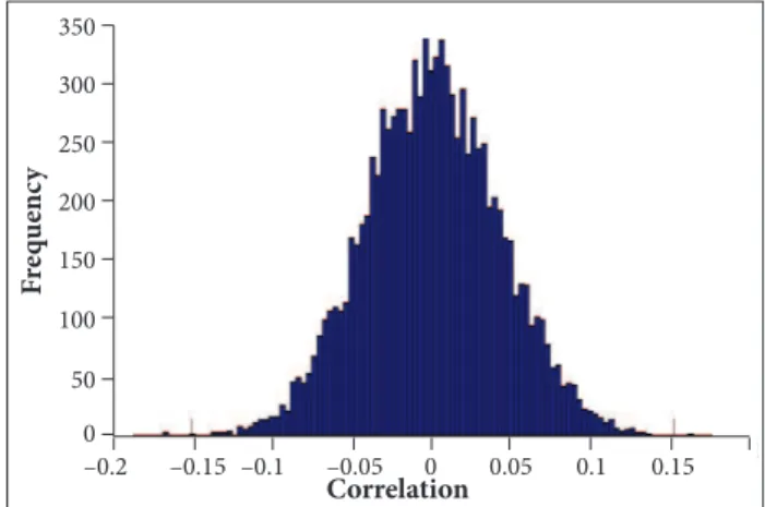
Figure 5 shows the result of the permutation test between SOI and the resulting monthly mean of zonal and meridional wind components from São Luís Airport surface station in the Maranhão State. The calculated result shows statistical evidence that the temporal series has a significant correlation with the 5% level of confidence interval. The correlation calculated (−0.230) is more displaced in the lower position of the tail of the distribution than the critical r value (−0.068) in the lower tail. The monthly mean wind can be associated with SOI variation signal, as the correlation was negative, showing that, in the months when SOI is negative (situation with El Niño), wind average would be higher.
Figure 5. Distribution of correlations between the monthly average of the wind and SOI.
DISCUSSION
t h e H m e t h o d c a n b e u s e d a s a n a l t e r n a t i v e t e c h n i q u e , a l l o w i n g t o s h o w t h a t S O I t i m e s e r i e s p r e s e n t s a l o n g - r a n g e m e m o r y w h i c h i s p e r s i s t e n t t h r o u g h o u t t h e l a g r a n g e s e r i e s . U s i n g F F T , a s i g n i i c a n t s i g n a l w a s o b t a i n e d , s u g g e s t i n g a p e r s i s t e n c e i n t h e t i m e s e r i e s . h i s m e t h o d o l o g y h a s s h o w n s t r o n g e v i d e n c e t h a t t h e H e s t i m a t i v e i s a b o v e 0.5, as the H value can represent a measure of the fractal dimension. A low fractal dimension presents greater coherence in time series and is more predictable; on the other hand, with high fractal dimension, it will have a behavior with less predictability.
he H calculation allows in its methodology to estimate a fractal dimension of SOI time series of about 1.78. his result can indicate chaotic behavior in SOI time series, thus quantifying the dependency or the sensitivity of the system to the initial ENSO conditions. Also, the ENSO irregularity can be viewed as a chaotic low-order process driven by the seasonal cycle.
CONCLUNDING REMARKS
he results show the importance of Ocean-atmosphere interaction, where there are non-linear interactions. Associated teleconnections efects create complex dynamics, inluencing and modulating the climatic indexes such as SOI.
In El Niño occurrence (negative SOI), there is a statistical correlation with the monthly mean wind and its maximum
monthly mean, as well as a tendency to inluence the average wind proile behavior near the surface, which operationally afects the ALC. El Niño characterizes a situation with stronger winds and predominant direction (east-northeasterly). Northward GRAD would intensify the negative precipitation anomalies in the northern-northeast Brazil.
he series features long-range memory behavior; therefore, this preliminary analysis indicates that autoregressive models can be used in the seasonal forecast for the Brazilian northeast and for trend studies with interest in seasonal variability range for the ALC. he knowledge of the SOI behavior and its association with wind variability allows a better prediction of wind intensity and, consequently, an improvement in the safety of ALC launch activities.
ACKNOWLEDGEMENTS
he authors thank the support of the Instituto de Aeronáutica e Espaço (IAE).
AUTHOR’S CONTRIBUTION
Conceptualization and Methodology, Corrêa CS. and Schuch DA; Writing – Review & Editing, Corrêa CS, Queiroz AP, Fisch G, Corrêa FN, and Coutinho MM.
REFERENCES
An SI, Wang B (2000) Interdecadal change of the structure of the ENSO mode and its impact on the ENSO frequency. J Clim 13(12):2044-2055. doi: 10.1175/1520-0442(2000)013<2044:ICOTSO>2.0.CO;2.
Andreoli RV, Kayano MT (2006) Tropical Paciic and South Atlantic effects on rainfall variability over northeastern Brazil. Int J Climat 26(13):1895-1912. doi: 10.1002/joc.1341.
Barnston AG, Ropelewski CF (1992) Prediction of ENSO episodes using canonical correlation analysis. J Clim 5(11):1316-1345. doi: 10.1175/1520-0442(1992)005<1316:POEEUC>2.0.CO;2.
Capotondi A (2013) El Niño-Southern Oscillation ocean dynamics: simulation by coupled general circulation models. In: Sun DZ, Bryan F, editors. Climate dynamics: why does climate vary? Washington: The American Geophysical Union. Geophysical Monograph, series 189.
Capotondi A, Wittenberg AT, Newman M, Di Lorenzo E, Yu JY, Braconnot P, Cole J, Dewitte B, Giese B, Guilyardi E, Jin FF, Karnauskas K, Kirtman B, Lee T, Schneider N, Xue Y, Yeh SW (2015) Understanding ENSO diversity. Bull Amer Meteor Soc
96(6):921-938. doi: 10.1175/bams-d-13-00117.1.
Chang P, Ji L, Wang B, Li T (1995) Interactions between the seasonal cycle and El Niño-Southern Oscillation in an intermediate coupled ocean-atmosphere model. J Atmos Sci 52(13):2353-2372. doi: 10.1175/1520-0469(1995)052<2353:IBTSCA>2.0.CO;2.
Collingridge DS (2013) A primer on quantitized data analysis and permutation testing. Journal of Mixed Methods Research 7(1):79-95. doi: 10.1177/1558689812454457.
Di Narzo AF (2013) tseriesChaos: analysis of nonlinear time series; [accessed 2017 Jul 5]. https://cran.r-project.org/web/ packages/tseriesChaos/index.html
Enield DB, Mayer DA (1997) Tropical Atlantic sea surface temperature variability and its relation to El Niño-Southern Oscillation. J Geophys Res 102(C1):929-945. doi: 10.1029/96JC03296.
Goldberger AL (1996) Non-linear dynamics for clinicians: chaos theory, fractals, and complexity at the bedside. Lancet 347(9011):1312-1314. doi: 10.1016/s0140-6736(96)90948-4.
Gonzalez RA, Andreoli RV, Candido LA, Kayano RA, de Souza RAF (2013) Inluence of El Niño-Southern Oscillation and Equatorial Atlantic on rainfall over northern and northeastern regions of South America. Acta Amaz 43(4):469-480. doi: 10.1590/S0044-59672013000400009.
Good PI (2005) Permutation, parametric and bootstrap tests of hipothesis. 3rd edition. New York: Springer-Verlag.
Hastings HM, Sugihara G (1993) Fractals, a user’s guide for natural sciences. Oxford: Oxford University Press.
Hegger R, Kantz H, Schreiber T (1999) Practical implementation of nonlinear time series methods: the TISEAN package. Chaos 9(2):413-435. doi: 10.1063/1.166424.
Hurst HE (1951) Long-term storage capacity of reservoirs. Transactions of the American Society of Civil Engineers 116(1):770-799.
Jin FF, Neeli JD, Ghil M (1996) El Niño/Southern Oscillation and the annual cycle: subharmonic frequency-locking and aperiodicity. Phys Nonlinear Phenom 98(2):442-465. doi: 10.1016/0167-2789(96)00111-X.
Kac M (1947) Random walk and the theory of Brownian Motion. Am Math Mon 54(7):369-391.
Kleinow T (2002) Testing continuous time models in inancial markets (PhD thesis). Berlin: Humboldt-Universität zu Berlin.
Mandelbrot B (1977) Fractals: form, chance and dimension. San Francisco: Freeman.
Mandelbrot B (1982) The fractal geometry of nature. San Francisco: Freeman.
Mandelbrot B (1983) Fractal and chaos. Berlin: Springer.
Marques RFC, Oyama MD (2015) Interannual variability of precipitation for the Centro de Lançamento de Alcântara in ENSO-neutral years. J Aerosp Technol Manag 7(3):365-373. doi: 10.5028/jatm.v7i3.477.
Newman M (2007) Interannual to decadal predictability of tropical and North Paciic sea surface temperatures. J Clim 20(11):2333-2356. doi: 101175/jcli4165.1
Rosenstein MT, Collins JJ, de Luca CJ (1993) A practical method for calculating largest Lyapunov exponents from small data sets. Phys Nonlinear Phenom 65(1-2):117-134. doi: 10.1016/0167-2789(93)90009-P.
Takahashi K (2011) ENSO regimes: reinterpreting the canonical and Modoki El Niño. Geophys Res Lett 38(10):L10704. doi: 10.1029/2011GL047364.
Temperton C (1985) Implementation of a self-sorting in-place prime factor FFT algorithm. Journal of Computational Physics 58(3):283-299. doi: 10.1016/0021-9991(85)90164-0.
Uvo CB, Repeli CA, Zebiak SE, Kushnir Y (1998) Relationships between tropical Paciic and Atlantic SST and northeast Brazil monthly precipitation. J Clim 11(4):551-562. doi: 10.1175/1520-0442(1998)011<0551:TRBTPA>2.0.CO;2.
Van Horne JC, Parker GGC (1967) The random-walk theory: an empirical test. Financial Analysts Journal 23(6):87-92. doi: 10.2469/faj.v23.n6.87.