How fast does a signal propagate through proteins?

Hui T. Young1,2, Scott A. Edwards4, Frauke Gra¨ter1,3*

1CAS-MPG Partner Institute and Key Laboratory for Computational Biology, Shanghai, P. R. China,2Graduate School of Chinese Academy of Sciences, Beijing, P. R. China, 3Heidelberg Institutes for Theoretical Studies gGmbH, Heidelberg, Germany,4College of Physics and Technology, Shenzhen University, Shenzhen, Guangdong, P. R. China

Abstract

As the molecular basis of signal propagation in the cell, proteins are regulated by perturbations, such as mechanical forces or ligand binding. The question arises how fast such a signal propagates through the protein molecular scaffold. As a first step, we have investigated numerically the dynamics of force propagation through a single (Ala)40 protein following a sudden increase in the stretching forces applied to its end termini. The force propagates along the backbone into the center of the chain on the picosecond scale. Both conformational and tension dynamics are found in good agreement with a coarse-grained theory of force propagation through semiflexible polymers. The speed of force propagation of~50A˚ ps21 derived from these simulations is likely to determine an upper speed limit of mechanical signal transfer in allosteric proteins or molecular machines.

Citation:Young HT, Edwards SA, Gra¨ter F (2013) How Fast Does a Signal Propagate through Proteins? PLoS ONE 8(6): e64746. doi:10.1371/journal.pone.0064746

Editor:Giorgio Colombo, Consiglio Nazionale delle Ricerche, Italy

ReceivedMarch 1, 2013;AcceptedApril 18, 2013;PublishedJune 6, 2013

Copyright:ß2013 Young et al. This is an open-access article distributed under the terms of the Creative Commons Attribution License, which permits unrestricted use, distribution, and reproduction in any medium, provided the original author and source are credited.

Funding:The authors thank the Klaus Tschira Foundation (http://www.klaus-tschira-stiftung.de) for funding. The funders had no role in study design, data collection and analysis, decision to publish, or preparation of the manuscript.

Competing Interests:The authors have declared that no competing interests exist.

* E-mail: frauke.graeter@h-its.org

Introduction

Mechanical force has long been recognized as one of the major factors that regulates biological function not only on the macroscopic level such as tissues and organs, but also on the microscopic level such as individual cells and proteins [1–3]. Cells and their constitutes are subjected to a constantly changing environment to which they are required to adopt in a dynamic and timely way. The dynamic response of a molecular system like a protein or protein complex to an external force has been extensively studied in experiments, simulations and theory [4–8]. While these processes of protein conformational changes or protein unfolding upon force application typically exhibit time scales from microseconds to seconds or even hours [9], the time scale of the force to propagate into the molecular structure is probably several orders of magnitude faster. The velocity of force propagation, i.e. the speed of sound, can be considered as an upper limit for the mechanical response of biomolecules, and thus is of fundamental interest in order to explore the dynamic consequences of external perturbations. One intriguing example is the helical fibers in hair cell bundles of vertebrate inner ear that serve as force transducers and are postulated to give rise to the exquisite frequency sensitivity ranging from 20 to 20 000 Hz and remarkably high dynamic range exceeds 100 dB [10–12].

Unfortunately, force propagation is inherently difficult to measure experimentally. Doing so not only requires excellent time resolution, one also has to either introduce force-sensitive probes into the molecular backbone [13] or resort to indirect and difficult to interpret measures such as force-induced heat dissipation [14]. However, the very same rapidity acting as a roadblock to experimental investigation pushes the subject of force propagation into the realm of atomistic molecular dynamics (MD) simulations, a technique that is limited to very short time scales,

but has proven useful for our understanding of protein dynamics [15]. In particular, a good agreement has been observed between experimental and simulated folding rates, suggesting the time scales of non-equilibrium processes investigated by MD simula-tions to be of a reasonable order of magnitude [16,17]. We take advantage of this fact by combining atomistic MD simulations of an (Ala)40 homo-polypeptide under external stretching force with

Force Distribution Analysis (FDA) [18], allowing us to track intramolecular forces with perfect temporal and spatial resolution (see Fig. 1).

Results

Tension Propagation from MD Simulations

After a sudden increase in the external force applied to the termini of (Ala)40 from fpre to fext, we monitored the tension

propagation into the center of the polypeptide by measuring the force between each pair of adjacent residues over time. While the MD simulations at the increased force offext were carried

out for 50 ps, we observed the inter-residue forces to equilibrate already within the first 10 ps, and thus restricted the analysis to this time window. As shown in Fig. 2a (diamonds), as expected, the increase in force between pairs of residues is highly non-linear and delayed towards the center of the chain. While the outer residue pairs show a rapid increase in inter-residue force within 1 ps, residue pairs located in the vicinity of the center of the chain exhibit a force increase significantly delayed on the picosecond time scale. A representative dynamic trajectory of (Ala)40 color coded by inter-residue forces is visualized in Movie

Bead-spring Model

Since protein dynamics are often treated within a linearized bead-spring framework [19,20], it is natural to assume that tension might propagate diffusively through the protein backbone, in the same way vibrational excitations do [14]. Assuming freely draining hydrodynamics, we solve the corresponding equations of motion.

k½x2(t){x1(t){‘0{(fext{fpre){fxx_1(t)~0

k½xiz1(t){2xi(t)zxi{1(t){fxx_i(t)~0, i~2. . .39

(fext{fpre){k½x40(t){x39(t){‘0{fxx_40(t)~0 xi(0)~(i{1)‘0,

ð1Þ

where f denotes the approximate bead friction coefficient f~6pgr, r&0:2nm the hydrodynamic radius of a single mono-mer,fprea low force at which the poly-alanine peptide was

pre-equilibrated, and fpre a higher external stretching force. By

matching the resulting stretching response x40(t){x1(t) to the

end-to-end distance for an intermediate stretching forcef, with fprevfvfext, in a corresponding MD force-extension curve

(Fig. 3), we determined both the backbone stiffness k~47Nm and the contour length per residue ‘0~0:344nm. The

force-extension profile for (Ala)40 (raw data in grey, averaged data in

blue in Fig. 3), obtained from additional MD simulations, gives the stretching force of the chain as a function of its end-to-end distance, and is directly comparable to experimental force-extension data.

Turning now to the time-dependent backbone tension fi(t)~fprezk(xiz1(t){xi(t)), we find that this severely

underes-timates the actual speed of tension propagation especially for the

inner most residues and intermediate time scales (not shown). One might argue that this is due to hydrodynamic cooperativity, as neighboring monomers move in unison, thus possibly shifting their effective friction coefficients towards the infinite-cylinder limit f&2pg(2r)=log (20)[21], thereby reducing friction by a factor of up to&5. This approximation, however, could only roughly bring our model in line with the MD data (Fig. 2a, Table S1 in File S1). Close to the center, even this manually corrected friction coefficient yields a time-dependent backbone tension that is too high at short times, but too low later on.

The likely reason behind this qualitative discrepancy is the inherently nonlinear stretching behaviour of polymers in thermal equilibrium. If the molecule was perfectly straight, then all the work done by the external stretching force went into pulling the polymer’s atomic constituents further apart, thus acting against powerful chemical binding potentials for which the harmonic approximation holds well beyond the external force levels considered here. As it is, however, Brownian forces always induce a certain amount of contour bending transverse to the polymer main axis, thus effectively shortening it in the longitudinal direction and providing a finite amount of ‘‘stored length’’ that is easily pulled out at forces far below those necessary to stretch the molecular backbone itself. A single stiffness chosen such as to correctly reproduce the overall longitudinal extension will thus always overestimate the actual stiffness, and thus the speed of tension propagation, at low stretching forces, Fig. 3.

Worm Like Chain (WLC) Model

Previous studies [22] have shown that polypeptides, like many other biopolymers, belong to the class ofsemiflexiblepolymers, rigid below a certain persistence length‘p but flexible on long scales

‘&‘p. Mathematically, semiflexible polymers are described by the

worm-like chainmodel, which yields an accurate expression for the

nonlinear force-extension relation [8] (presuming zero backbone extensibility),

f‘p

kBT

~Rz

Lz

1 4(1{Rz=L)2

{1

4, ð2Þ

whereLdenotes the total polymer length andRzits longitudinal

extension. Previous experimental measurements of‘p&1nmshow

that we are very close to full extension, f&kBT=‘p&4pN,

allowing us to simplify the force-extension relation as follows,

Rz

L~1{ 4f‘p

kBT

{1=2

: ð3Þ

Meanwhile,f is large enough to stretch the backbone, which we may regard as a linear spring, f~_k(L{_L(f~₀₎₎, i.e. the full force-extension relation for strong contour straightening and weak backbone stretching reads.

Rz~L0 1{ 4f‘p

kBT

{1=2

" #

zf

k, ð4Þ

whereL0 denotes the molecule’s natural contour length, i.e., the

longitudinal extension of its energetic ground state. By fitting the above expression to our force-extension data, we obtain

‘p&0:7nm,L0&14:7mmandk&4:2Nm{1. Raising the external

force from fpre to fext thus stretches the backbone by &2:4%,

Figure 1. Force propagation along a polypeptide in water.(a)

After first equilibrating an (Ala)40 polypeptide under a relatively low

stretching force of fpre~167pN applied to both termini of the polypeptide, we then suddenly increase the stretching force by a factor of 10 tofext. As the polymer is straightened, backbone tension propagates from the two termini into the center of the chain. (b) Structure used in the MD simulation. The (Ala)40 polypeptide is

surrounded by explicit solvent molecules. A constant force,fpreorfext is applied to the terminal C-aatoms, and the end-to-end distanceRof the peptide is measured.

whereas the strain caused by contour straightening is more than twice as large as the harmonic contribution,

DRstraightening z

L0 ~

ffiffiffiffiffiffiffiffiffi

kBT

4‘p s

f{1=2 pre {f

{1=2 ext

&6:2%: ð5Þ

In contrast to the linear bead-spring model, the Wormlike Chain gives rise to very complex short-time behaviour that can only be accounted for by explicit consideration of the nonequilibrium relaxation behaviour of mechanical bending modes [23–26]. Fortunately, in the limit of ‘‘long’’ times (in our case anything beyond t~00:01ps) these quickly fluctuating bending modes adapt quasistatically to changes in the backbone tension f(s,t), thus allowing us to generalize the above static force-extension relation to spatially and temporally varying tension profilesf(s,t),

‘~ 1{

ffiffiffiffiffiffiffiffiffiffiffiffiffiffiffiffiffi

kBT

4f(s,t)‘p s

zf(s,t) kL

" #

‘0, ð6Þ

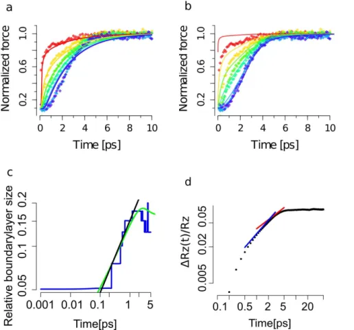
Figure 2. Tension propagation from MD simulations and comparison to dynamic bead-spring and semiflexible chain models.(a)

Tension evolution as predicted by a bead-spring model (colored curves) fitted to the tension in Ala40as obtained from MD simulations (colored

diamonds). Coloring red, yellow, green yellow, blue and purple show residue pairs 1–2, 4–5, 7–8, 10–11, 15–16 and 20–21, respectively. A manually reduced friction coefficient was used to map the WLC model and numerical results. We note that here forces were averaged over 100 fs time periods for clarity. (b) Tension evolution from the dynamic WLC model (colored curve) fitted to the tension in Ala40as obtained from MD simulations (colored

diamonds). Coloring and averaging as in (a). (c) Boundary layer sizelE(t)relative to the contour lengthLobtained from MD simulations shown inblue. Numeric solution to the dynamic WLC model prediction in greenandy!x1=2 _{growth law inblack. (d) ExtensionDRz=Rzshown asblack dots}

compared to two growth laws,y!x3=4_inblueandy!x1=2_inred.

doi:10.1371/journal.pone.0064746.g002

Figure 3. Force-Extension curve of the (Ala)40 chain (grey dots).

where‘denotes the length of an infinitesimal piece of polymer (of rest length‘0).

The corresponding changes in local strain Lt‘ determine the

longitudinal velocity gradientsLsvE~Ls(fELsf)(for further details

please refer to [23–26]), thus furnishing us with a closed partial differential equation for the time- and space-dependent tension profile,

L2_sf~f_Eff_(s,t) 1 4

ffiffiffiffiffiffiffiffiffi

kBT

‘p s

f(s,t){3=2z1=(kL)

!

, ð7Þ

valid for t&kBT‘pf\=(fprefext)*0:01ps [25] which we solve

under the given initial and boundary conditions f(s,0):fpre, f(0,t):f(L,t):fext. Figure 2b shows the results from the dynamic

WLC model for the time-dependent inter-residue forces as obtained from MD simulations (same as Figure 2a). The agreement with our MD data is much improved, especially deep within the chain where forces remain within the regime of nonlinear extensibility for several (Table S1 in File S1).

We also quantified and compared theboundary layer as it was defined within the dynamic WLC model in [27]. Following the sudden increase of the external forcefext, the polymer stretches its

contour within a growing boundary layer lE(t). Only within boundary layers, the thermally undulated contour is straightened while in the bulk of the chain tension stays in their originalground

statedefined by fpre. Practically, the boundary layer is defined as

the segment of the polymer such that its tension f(lE)~(fextzfpre)=2. The boundary layer growth in the (Ala)40

chain relative to its contour lengthlE(t)=L(t)is compared to the model prediction in Figure 2c. We extracted the characteristic parametertEL= 1.2 ps, which marks the crossover from the tension

propagation into the relaxation phase. In consistence with the

analytical model put forward in [25], for tk=f\&(fextfpre) {1

, the boundary layerlE(t)=L(t)scales asl1=2

p fpre1=4(fextt)1=2before two

boundary layers from both ends meet each other. Here,k~kBT‘p

and f\ are the bending stiffness and the friction coefficient for

transverse motion, respectively. We note that the stair wise appearance of the boundary layer growth in our simulations is due to the discrete nature of the polypeptide chain.

Another observable that we compared to the dynamic WLC model prediction is the change in chain extension DRz(t). As

shown in Figure 2d, its growth is nonlinear and showed a crossover from DRz!t3=4 into DRz!t1=2, which corresponds to the

transition from the tension propagation regime into the relaxation regime [25].

Discussion

Through Molecular Dynamics simulations of polyalanine, we have shown that coarse-grained models of semiflexible polymer dynamics yield an accurate description of tension propagation and stretching dynamics even in peptide-sized macromolecules, thus providing a reliable theoretical framework on all relevant length scales.

In a bulk material, the longitudinal signal propagation is given by the Newton-Laplace equation, c~pffiffiffiffiffiffiffiffiffiffiY=r, where r is the density of the material and Y is the Young’s modulus. Our calculations allow to estimate the signal propagation speed for the nanometer-sized single molecule chain of poly-alanine. With a Young’s modulus of 13 GPa at a constant force offpre= 166 pN

and arof 507.8 kg m23_{derived from van der Waals volume, we} obtain a speed ofc= 51 A˚ :ps21_.

Alternatively,ccan be estimated from the propagation regime characteristic time scale tE_L= 1.2 ps in the non-equilibrium MD simulations. Considering that the signal only travels through half the chain lengthRz, the effective signal propagation speedfcff^0gg

is given by c0~Rz=2=tEL= 56 A˚ ? ps21. This estimate

quantita-tively agrees with the estimation from the Newton-Laplace equation, suggesting the theory for macroscopic bulk materials to hold at the level of discrete single molecular chains.

The longitudinal mechanical signal propagation speed we determined here for a stretched peptide is roughly two times of the speed of sound in myoglobin obtained previously [28] and 1.5 times of the value reported for a densely packed b-sheet rich proteins in another study [29]. In a stretched peptide, mechanical force almost exclusively transfers through the backbone while in the case of myoglobin or b-sheet rich proteins it also transfers through a softer network of hydrogen bonds and other non-covalent molecular contacts, which apparently slows down the propagation of forces relative to their transfer through covalent bonds. Mechanical signal propagation plays a pivotal role in protein allostery, which is known to involve much longer time scales from microseconds onwards, but could be envisioned to be partly determined by transmission through either faster backbone or slower non-covalent forces, or a combination thereof. How the picosecond time scale of force propagation through our simplistic single-chain system relates to the dynamics of signal transmission through larger allosteric proteins or molecular machines remains to be resolved.

Methods

Molecular Dynamics Simulations

Our simulation encompasses a triclinic box of size 6|6|40 nm with periodic boundary conditions containing besides the (Ala)40 peptide approximately 47000 SPC water molecules [30].

We first perform 2000 energy minimization steps using a steepest descent algorithm, followed by 1 ns of MD simulation to equilibrate the solvent. During solvent equilibration, all protein atoms are held in place by harmonic potentials of stiffness kpr~1000 kJ mol21 nm2. Next, we remove the artificial

constraining potentials and turn on the pre-stretching force, corresponding to linear potentialsUpre~+fprezacting on residues

1 and 40, respectively. Another 500ps of MD simulation ensure complete tension equilibration within the peptide. We then increase the external stretching force by a factor of 10 and record all atomic trajectories (with a time resolution of 1fs) during the following 50ps of simulation time.

Using the Force Distribution Analysis (FDA) method imple-mented based on Gromacs [18], we also record the vectorial forces between each pair of atoms within cut-off distance of each other, again with a time resolution of 1 fs. From this we obtain the sought-after backbone tension by summing all forces between adjacent residues and projecting onto the polymers main axis^eez.

All simulations are carried out in GROMACS 4.5.4 [31] using the OPLS/AA force field [32] and a 1.0 nm cutoff for non-bonded interactions. Within the 1.0 nm distance, electrostatic interactions are calculated explicitly, while longer ranged electrostatic interac-tions are evaluated using the Particle Mesh Ewald summation method [33]. Simulations are performed within the NpT ensemble, where temperature is kept constant at 300K by a Nose-Hoover thermostat coupling with a time constant oftT~0:1

ps [34] and the pressure constraint p~1 bar is enforced by a Parrinello-Rahman barostat coupling with tP~1:0 ps and

For a single nonequilibrium simulation, the magnitude of tension fluctuations measures approximately 6000 pN (Fig. S1a in File S1), thus dwarfing the deterministic average force by a factor of almost 4: 1. To arrive at a reasonable signal-to-noise ratio, we average over 100 independent trajectories following the same force-jump protocol, resulting in standard errors of the mean in the range of 20–50 pN (Fig. S1b in File S1), i.e. below the average differences between residue pairs along the chain and in time. We also measure the static force-extension relation by attaching harmonic potentials of stiffness 500 kJ mol21_nm2_{to the terminal} residues and moving them outwards at different constant speeds between 0.5 and 10 nm/ns (constant velocity pulling). The resulting curves are velocity-independent, proving that the pulling velocity is slow enough for backbone tension to equilibrate quasistatically.

Supporting Information

File S1 Detailed model fitting parameters.

(PDF)

Movie S1 Dynamics of tension propagation after the jump to a high stretching force mapped onto the stretched (Ala)40 chain.Elevated force propagates from both ends of the peptide into the central region. The color code from bluetoredindicates lowest to highest inter-residue forces. Only the first10psare shown.

(MOV)

Acknowledgments

We thank Sebastian Sturm for the many intensive discussions, assistance with the theoretical models, and constructive comments on the manuscript, and Dr. Benedikt Obermayer for providing us with his numerical solver for the full (non-quasistatic) theory of tension propagation in semiflexible polymers.

Author Contributions

Conceived and designed the experiments: FG. Performed the experiments: HTY. Analyzed the data: HTY SAE FG. Contributed reagents/materials/ analysis tools: HTY SAE. Wrote the paper: HTY FG.

References

1. Gomez GA, McLachlan RW, Yap AS (2011) Productive tension: force-sensing and homeostasis of cell-cell junctions. Trends Cell Biol 21: 499–505. 2. Husson J, Chemin K, Bohineust A, Hivroz C, Henry N (2011) Force generation

upon T cell receptor engagement. PLoS ONE 6: e19680.

3. DuFort CC, Paszek MJ, Weaver VM (2011) Balancing forces: architectural control of mechanotransduction. Nat Rev Mol Cell Biol 12: 308–319. 4. Grandbois M, Beyer M, Rief M, Clausen-Schaumann H, Gaub H (1999) How

strong is a covalent bond? Science 283: 1727–1730.

5. Smith D, Babcock HP, Chu S (1999) Single-polymer dynamics in steady shear flow. Science 283: 1724–1727.

6. Isralewitz B, Gao M, Schulten K (2001) Steered molecular dynamics and mechanical functions of proteins. Curr Opin Struct Biol 11: 224–230. 7. Samuel J, Sinha S (2002) Elasticity of semiflexible polymers. Phys Rev E 66:

50801.

8. Marko J, Siggia E (1995) Stretching dna. Macromolecules 28: 8759–8770. 9. Dror RO, Dirks RM, Grossman JP, Xu H, Shaw DE (2012) Biomolecular

Simulation: A Computational Microscope for Molecular Biology. Annu Rev Biophys 41: 429–452.

10. Kachar B, Parakkal M, Kurc M, Zhao Y, Gillespie PG (2000) High-resolution structure of hair-cell tip links. Proc Natl Acad Sci USA 97: 13336–13341. 11. Nam JH, Fettiplace R (2008) Theoretical Conditions for High-Frequency Hair

Bundle Oscillations in Auditory Hair Cells. Biophys J 95: 4948–4962. 12. Gillespie PG, Mu¨ller U (2009) Mechanotransduction by hair cells: models,

molecules, and mechanisms. Cell 139: 33–44.

13. Shroff H, Reinhard BoM, Siu M, Agarwal H, Spakowitz A, et al. (2005) Biocompatible Force Sensor with Optical Readout and Dimensions of 6 nm3. Nano Lett 5: 1509–1514.

14. Botan V, Backus EHG, Pfister R, Moretto A, Crisma M, et al. (2007) Energy transport in peptide helices. Proc Natl Acad Sci USA 104: 12749–12754. 15. Karplus M, McCammon JA (2002) Molecular dynamics simulations of

biomolecules. Nat Struct Biol 9: 646–652.

16. Snow CD, Nguyen H, Pande VS, Gruebele M (2002) Absolute comparison of simulated and experimental protein-folding dynamics. Nature 420: 102–106. 17. Snow CD, Sorin EJ, Rhee YM, Pande VS (2005) How well can simulation

predict protein folding kinetics and thermodynamics? Annu Rev Biophys Biomol Struct 34: 43–69.

18. Stacklies W, Seifert C, Gra¨ter F (2011) Implementation of force distribution analysis for molecular dynamics simulations. BMC Bioinformatics 12: 101.

19. Tirion M (1996) Large Amplitude Elastic Motions in Proteins from a Single-Parameter, Atomic Analysis. Phys Rev Lett 77: 1905–1908.

20. Takada S (2012) Coarse-grained molecular simulations of large biomolecules. Curr Opin Struct Biol 22: 130–137.

21. Batchelor GK (1970) Slender-body theory for particles of arbitrary cross-section in Stokes flow. J Fluid Mech 44: 419–440.

22. Schuler B (2005) Polyproline and the "spectroscopic ruler" revisited with single-molecule fluorescence. Proc Natl Acad Sci USA 102: 2754–2759.

23. Hallatschek O, Frey E, Kroy K (2007) Tension dynamics in semiflexible polymers. I. Coarse grained equations of motion. Phys Rev E 75: 031905. 24. Hallatschek O, Frey E, Kroy K (2007) Tension dynamics in semiflexible

polymers. II. Scaling solutions and applications. Phys Rev E 75: 031906. 25. Obermayer B, Hallatschek O, Frey E, Kroy K (2007) Stretching dynamics of

semiflexible polymers. Eur Phys J E 23: 375–388.

26. Obermayer B, Mo¨bius W, Hallatschek O, Frey E, Kroy K (2009) Tension dynamics and viscoelasticity of extensible wormlike chains. Phys Rev E Stat Nonlin Soft Matter Phys 80: 040801.

27. Hallatschek O, Frey E, Kroy K (2005) Propagation and Relaxation of Tension in Stiff Polymers. Phys Rev Lett 94: 77804.

28. Yu X, Leitner DM (2003) Vibrational Energy Transfer and Heat Conduction in a Protein. J Phys Chem B 107: 1698–1707.

29. Xu Z, Buehler MJ (2010) Mechanical energy transfer and dissipation in fibrous beta-sheet-rich proteins. Phys Rev E 81: 061910.

30. Berendsen H, Postma J, Van Gunsteren WF, Hermans J (1981) Interaction models for water in relation to protein hydration. Intermolecular Forces 11: 331–342.

31. Hess B, Kutzner C, van der Spoel D, Lindahl E (2008) GROMACS 4: Algorithms for Highly Efficient, Load-Balanced, and Scalable Molecular Simulation. J Chem Theory Comput 4: 435–447.

32. Jorgensen WL, Tirado-Rives J (1988) The OPLS [optimized potentials for liquid simulations] potential functions for proteins, energy minimizations for crystals of cyclic peptides and crambin. J Am Chem Soc 110: 1657–1666.

33. Essmann U, Perera L, Berkowitz ML, Darden T, Lee H, et al. (1995) A smooth particle mesh Ewald method. J Chem Phys 103: 8577.

34. Hoover W (1985) Canonical dynamics: equilibrium phase-space distributions. Phys Rev A 31: 1695–1697.