Applications of Spatial Data Using Business Analytics Tools
Anca Ioana ANDREESCU, Anda VELICANU, Daniela MITROESCU Economic Informatics and Cybernetics Department, Academy of Economic Studies,
Bucharest, ROMANIA
[email protected], [email protected], [email protected]
This paper addresses the possibilities of using spatial data in business analytics tools, with emphasis on SAS software. Various kinds of map data sets containing spatial data are presented and discussed. Examples of map charts illustrating macroeconomic parameters demonstrate the application of spatial data for the creation of map charts in SAS Enterprise Guise. Extended features of map charts are being exemplified by producing charts via SAS programming procedures.
Keywords: spatial data, business analytics, SAS system, map charts
Introduction
Historically speaking, since the ‘70, methods of statistical calculation and data processing have begun to change with the introduction of integrated statistical packages. They allow users to perform one or more statistical procedures on a single set of data stored in a file format standard. Processing and data management have been hardly started and cumbersome and mapping packages were missing from the standard system [1]. Given the growing necessity of representing geographical distributed information we will discuss in the paper how analytics tools deal with geographic data and allow graphical descriptions based on this data.
2 Spatial data structure
The spatial data (geographical data) emerged from the need to work and process geographical data like points, lines, polygons, three-dimensional geometric objects representing real world objects. Spatial locating this data can be bi-or tri-dimensional, depending on its type and the information available. Such a two-dimensional level can indicate the latitude and longitude coordinates or x and y coordinates of a given finite area and a three-dimensional level can specify latitude, longitude and height / altitude or the x, y and z coordinates in a given finite area. Examples of spatial objects are
cities, buildings, rivers, touristic points of interest etc. This article will mainly deal with issues regarding bi-dimensional spatial databases.
Spatial objects consist of points, lines, surfaces, volumes and objects of higher dimensions that are frequently used in computer aided design applications, cartography, GIS, etc. They are described by spatial attributes (length, configuration, perimeter, area, volume, etc.) and by non-spatial (common) attributes (the creating date, ownership, membership of a superior structure, etc.). The values of spatial attributes of these objects represent spatial data.
Objects in the real world can be divided into two categories: discrete objects (a house) and continuous fields (rainfall or altitude).
Geographic data represent real world objects (roads, soil, elevation) by storing data with two or three measurable dimensions relative to a Cartesian coordinate system or latitude-longitudinal system.
Spatial data can be divided into point data and regional data. The point data is completely characterized by its location in a multidimensional space. It can come directly from measurements or can be rendered in order to be more easily stored and retrieved. Regional data is characterized by location (a fixed point in a region) and destination (a line in 2D or a 3D surface).
Spatial data are also those of a certain rank (e.g. "Cities in Europe"), approaches data (e.g. "Three close lakes in Romania"), junction data (e.g. "Pairs of cities in Romania located at 50 km of each other ").
Spatial data structure is specific for storing, querying and processing the geometric information. This allows us to provide the necessary information for a database management system (DBMS) so that it can follow the spatial data model. In general, a geographic data structure must allow the representation of three components:
• data on the geography of objects
(points, lines, polygons);
• date on objects’ attributes (name,
description);
• images (used usually as background
maps or as symbolic representation of objects – e.g. a green cross for pharmacies, a triangle for campsites, a tree for forests etc.).
Raster and vector data models based on spatial data representation are considered to be dual by [2].
The two main models used for storing such data - raster and vector - are detailed in [3]. Raster model is based on partitioning the areas and the vector model works with points, lines and
polygons that describe the geometry of a spatial object. [4] identifies five levels of significance for the representation of real world entities in data structures that can be implemented in the computer:
• entities level;
• objects level;
• conceptual level;
• raster and vector level;
• data structures level (implementation
level).
The difference between entity and object, shown by [4], is that entities can be seen as phenomena that have no clear physical boundary, while the objects are defined by dimensional attributes (length, width, volume).
At a conceptual level, the objects acquire attributes such as distance, coordinate system, and topology. Raster or vector level determines how objects are represented as spatial data. The implementation level depends on the DBMS through which spatial data is stored according to available data structure and the specialized spatial database (SDB).
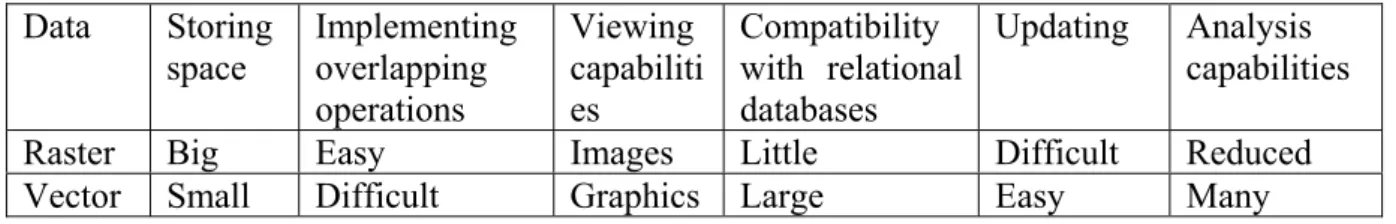
Table 1 presents a comparative analysis of both data types, in terms of characteristics such as storage, operations’ implementation, compatibility with relational databases, updating and analysis capabilities.
Table 1. Comparative analysis of raster and vector data
In the table above it can be noticed that using raster data has advantages like easy implementation of overlapping operations, methods of rendering images, while using vector data requires less storage space, methods of rendering graphics, large compatibility with relational databases, ease to update and many analysis facilities.
As illustrated in paper [5], creating a professional looking Map Chart in SAS Enterprise Guide is a simple process that has gotten easier with each release of the software. As long as data that can be joined to a map dataset, high quality maps can be created. It only requires one task and two datasets in the simplest form.
Data Storing space
Implementing overlapping operations
Viewing capabiliti es
Compatibility with relational databases
Updating Analysis capabilities
Raster Big Easy Images Little Difficult Reduced
The coordinate system, also called spatial reference system, is another important notion when talking about spatial data. The coordinate system is a mean of allocating the coordinates to a location and establishing relationships between sets of such coordinates. This allows interpreting a set of coordinates as a representation of a location in the real world. Each spatial data has an associated coordinate system. The coordinate system can be:
• with a geo-reference (geodesic,
depending on a certain representation of Earth);
• without a geo-reference (Cartesian,
not depending on a certain representation of Earth).
If the coordinate system is geodesic, then it has an associated default unit of measurement (e.g. meters), but can have automated transformation of data into other units (e.g. miles). Spatial data can be associated with Cartesian, geodetic (geographical), projected or local coordinate system.
Cartesian coordinates are those which measure the position of a point along the axes that are perpendicular in the origin, representing two-dimensional or three-dimensional space. If a coordinate system is not explicitly associated with geometry, it is assumed that the geometry is in Cartesian coordinate system.
Geodetic coordinates are longitude and latitude, closely related to spherical polar coordinates and are defined relative to a certain geodesic data.
Projected coordinates are plane Cartesian resulting from performing a mathematical mapping from a point on the Earth's surface onto a plane. There are many such mathematical mappings.
Local coordinates are Cartesians in a non-geodetic coordinate system. They are often used for CAD (Computer Aided Design).
When performing operations on spatial data a Cartesian model or a curvilinear pattern must be used, according to the
coordinate system associated with the data. In SAS Enterprise Guide the coordinate system can be defined after the spatial data is imported from a database or a data file (xls, html etc.).
For systems that store and process spatial data in spatial databases it results in a number of advantages, primarily due to their specialization (dedicated system). Thus, the general advantages of working with geographic data are shown in [6]:
• precision in representing the data and
processing it;
• creating and using specific libraries
(information structuring, using standards, interchanging information);
• possibility to update information;
• quick access to information (due to
flexible organizing criteria and to fast working speed of the equipment);
• easily, precise and unlimited
reproducing of graphic material (paper copies can be obtained quickly and also spreadsheets and scale drawings can be done considering the user’s choice);
• adaptability to evolution of informatics
technologies.
If data to be used is not yet in digital format, there are several techniques by which spatial information can be obtained.
Thus, maps can be digitized or drawn with the mouse for collecting the coordinates of various items. Scanning with electronic devices can also help convert the lines and points on a map into digital data.
3 Producing map graphs with SAS Enterprise Guide
Being one of the largest software producers for statistics and business analytics in the world, SAS paid particular attention to the representation of spatial data in its solutions. SAS Enterprise Guide is the Graphical User Interface (GUI) that helps to exploitation and dynamic publication in a Microsoft Windows client application. SAS interface is the preferred solution for business analysts, programmers and statisticians.
SAS means analysis and data management, a series of procedures and programming capabilities. An important feature offered by SAS statistical processing of cartographic data based on geographically and able to juggle with these statistics to obtain cartographic works. Map coordinates are stored in tables provided to streamline the process. So, in order to create a map, the user needs tables for storing the owned information that will be implemented through a mapping process. Further, the imported data are joined (intersection) in Enterprise Guide with the coordinates provided by the system, and this will generate the final mapping product. SAS offers users the possibility to choose the type of map produced from a variety of devices widely available, simple maps, maps with parameter chosen by the user, the possibility to redefine the geographical regions, the possibility to choose maps colors [7].
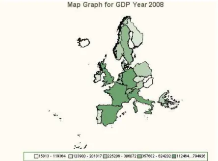
The following paragraphs will present the process steps necessary to create a cartographic work. The analyzed data are actual values of macroeconomic indicators, studied for the countries of the international economic organizations, the Organization for Economic Co-operation and Development (OECD).
The first step is to import tables containing data. Different formats of tables can be imported, including xls, mdb, csv and html. In the example, we
have chosen to import tables in mdb format. To create a parameter map with all the values we need in a single table of indicators including Gross Domestic Product (GDP), Net Domestic Product (NDP) and UNEMPLOYMENT, so the tables imported have been joined. To join two or more tables Query Builder tool have to be used and one can choose the type of join (manually or automatically).
To create a map using SAS Enterprise Guide 4.2, we need to get the geographic
coordinates owned by the system in the map
library. A join was made between the imported table, which contains indicators for each country, and the table with the coordinates of the system. Next, a map is created for the data we get by processing imported tables. As settings we can choose the type of the map (Choropleth, Riser and Prism), data sources, appearance, titles and other properties. To set up a map with a parameter that can be chosen at runtime, a variable that will contain the list of indicators was created. Creating a map in SAS Enterprise Guide 4.3 is even easier than in version 4.2 of this product. Briefly, the key element to create a Map Chart is to making sure your data and the map file have a commonly named variable on which to join. As mentioned before, earlier versions required to use the Query Builder task to join your data to the shape or map file. In 4.3, this is done automatically. In order to create a basic Map Chart, the user must only provide data with a geographic variable and an analysis variable [5].
for that geographical area. The same information as in figure 1 is represented in this chart.
Figure 1. Choropleth map chart
Figure 2. Riser map chart
4 Extended features of map graphs in SAS
Map graphs produced by SAS Enterprise Guide are static and their lone purpose is to display information. New features within SAS/GRAPH allow for the creation of maps with dynamic features
like drill-down areas, pop-ups and animation. This implies writing SAS code for achieving such features.
information associated with each map area. In this regard, two data sets will be used to create a map graph which will display the population density for all Romanian counties. The first (named
romanian_dens), containing the response data set, has three variables: ID – identification number for a county, County_name and Density – the density of population per square kilometer in the year 2006, information retrieved from [8]. The second data set (named
Romania) is the Romanian shape file provided by SAS system and located in the map library.
The SAS code from the program below generates a map graph of the Romanian population density in the form of an html type file.
*** Section 1 - create a format to display county name;
data county_fmt (keep=fmtname start label)
/ view=county_fmt;
retain fmtname 'countyname'; set romanian_dens
rename=(ID=start county_name=label)); run;
proc format cntlin=county_fmt; run;
*** Section 2 - set graphics and output options;
goptions reset=all device=activex xpixels=700 ypixels=500; ods listing close;
ods html file = 'c:\romania.html'; title ‘ROMANIAN POPULATION
DENSITY By COUNTY, 2006’;
footnote j=r 'Pop-ups in Map Graph'; *** Section 3 - define graph
parameters;
proc gmap data=romanian_dens map=maps.romania;
id ID;
choro density / levels=all nolegend; format ID countyname.;
label ID = 'COUNTY'; run;
The following paragraphs explain how the SAS language features were used in the source code presented above.
In Section 1, the data step creates a user
format (county_fmt) that will be used in
proc gmap command to display information associated with each Romanian county. This will be done starting from the
romanian_dens data set (specified in the set
command). The keep flag determines
whether or not a variable is written to the output data set. The specified variables will be the only variables in your output data set
[9]. The view option tells SAS to compile,
but not to execute, the source program and to store the compiled code in the input DATA step view that is named in the option [10]. Retain flag is used to prevent fmtname
variable from being reset to missing at the top of the data step. This makes it a vital tool for passing information from one observation to another.
An important feature of SAS language is the ability to create user-defined formats starting from a specially constructed SAS
data set. This can be done using the proc
format option cntlin= (control in) that permits the user to name the data set (or data view in our case) which will be used. Control input data set require a minimum of
three variables, named ftmname (the format
name), start (a single value that will be
formatted) and label (information to be
displayed) [11].
Section 2 has the roles of resetting the graphics options to default values, selecting the JAVA device driver and setting the image size. Also, using the Output Delivery
System (ods) a html file is generated and
characteristics of this output type (title and footnote) are being defined.
Section 3 involves the actual construction of
the graph through the gmap procedure. The
GMAP procedure produces two-dimensional (choropleth) or three-dimensional (block, prism, and surface) maps that show variations of a variable value with respect to an area [12]. The only type of map graph that SAS can create using only code, not Enterprise Guide tasks is the surface graph
type. Main parameters of gmap proc are
response data set (data), map data set (map), variable that determines the color intensity
of the geographic areas (id) and type of
the resulting map, as it can be seen in Figure 3, information about each area (the value of the ID variable and the value of the variable in the CHORO statement) appear in pop-up box as the
mouse cursor is moved over the map. In addition, the user could alter the appearance of the map if the right mouse button is clicked anywhere on the map surface.
Figure 3. Map chart with pop-up features
5 Conclusions
The possibility to represent spatial data in statistics and analytics software tools is an important characteristic in the context of the new economy, mainly due to globalization and geographic distribution of organizational units in various economic areas. SAS software offers big support in this regard, by letting users to manipulate different kind of spatial data and to create map graphs. Besides the support offered through the map library, additional maps can be found on the SAS Maps Online page available at [13]. Besides this, a connection with professional spatial analysis tools can be made using, for example, SAS Bridge for ESRI to access ArcGIS files.
References
[1] G. B. Meehan, Statistical Mapping
Capabilities and Potentials of SAS, Institute for Research in Social Science, University of North Carolina, 1982
[2] D. Peuquet, Representations of Geographic Space: Toward a Conceptual Synthesis, Annals of the
Association of American Cartographers, Nr. 78 (3), 1988, pp. 375-394.
[3] Geographic information system
http://en.wikipedia.org/wiki/Geographic_ information_system#Data_representation
[4] R. McMaster, L. Barnett, A spatial-object level organization of
transformations for cartographic generalization, Proceedings of the International Symposium on Cmputer – Assisted Cartography Auto-Carto 11, 1993, pp. 386-395.
[5] S. R. Thompson, Easier than You Think:
Creating Maps with SAS Enterprise Guide, SAS Global Forum 2011, Las Vegas, Nevada, USA,
http://support.sas.com/resources/papers/ proceedings11/311-2011.pdf
[6] M. Băduţ , Soluţie pentru proiectarea si administrarea întreprinderilor - O tripletă de încredere: MicroStation - MicroStation GeoGraphics - PlantSpace, PC World Romania, nr 7, 1997, pp. 12
[7] M. Zdeb, Creating Maps with
http://www2.sas.com/proceedings/sug i29/toc.html
[8] Density of Romanian population,
http://enciclopediaromaniei.ro/wiki/In dex:Jude%C5%A3e#cite_note-2
[9] An Introduction to SAS Data Steps,
http://www.ssc.wisc.edu/sscc/pubs/4-18.htm
[10] DATA Step Views,
http://support.sas.com/documentation/ cdl/en/lrcon/62955/HTML/default/vie wer.htm#a001278887.htm
[11] R. Cody, Learning SAS by Example: A
Programmers Guide, SAS Institute Inc., Cary, USA, 2007
[12] SAS GMAP Procedure,
http://support.sas.com/documentation/cdl /en/graphref/63022/HTML/default/viewe r.htm#overview-gmap.htm
[13] SAS Maps Online,
http://support.sas.com/rnd/datavisualizat ion/mapsonline/
Anca Ioana ANDREESCU is university lecturer in Economic Informatics and Cybernetics Department, Academy of Economic Studies of Bucharest. She published over 15 articles in journals and magazines in computer science, informatics and business management fields, over 20 papers presented at national and international conferences, symposiums and workshops and she was member in over nine research projects. In January 2009, she
finished the doctoral stage, the title of her PhD thesis being: The
Development of Software Systems for Business Management. Her interest domains related to computer science are: business rules approaches, business analytics, requirements engineering and software development methodologies.
Anda VELICANU has graduated the Faculty of Economic Cybernetics, Statistics and Informatics of the Bucharest Academy of Economic Studies, in 2008. She has a PhD in Economic Informatics and since January 2009 she is a Pre-Assistant Lecturer. She teaches Database, Database Management Systems and Software Packages seminars at the Economic Cybernetics, Statistics and Informatics Faculty. Her research activity can be observed in the following achievements: 11 diplomas, 2 scientific awards, 13 proceedings, 7 articles published in scientific reviews, 4 research contracts, 3 books and 1 research grant. She is a member of INFOREC professional association, secretary of the “Database Systems Journal”. Her scientific fields of interest include: Databases, Database Management Systems, Spatial Databases, Programming, Information Systems.