American Journal of Applied Sciences 5 (8): 1023-1028, 2008 ISSN 1546-9239
© 2008 Science Publications
Corresponding Author: Dr. Mohamed Khaled Omar, Faculty of Engineering and Technology, Multimedia University, Jalan Ayer Keroh Lama, 75450 , Malaysia, Tel: +604-2523313
Two Mathematical Modeling Approaches for Integrating
Production and Transportation Decisions in the Process Industry
Mohamed.K. Omar and A. Ajitha
Centre of Computer Aided Design and Knowledge Manufacturing (CCADKM),
Faculty of Engineering and Technology, Multimedia University-Melaka Campus,
Jalan Ayer Keroh Lama, 75450 Melaka, Malaysia
Abstract: In this study we focus on coordination of the production planning of finished products and intermediate products in the process industry. The problem consists of two manufacturing facilities with similar production environment, one producing the intermediates and the other producing end products that are separated by a distance. There is transportation between the facilities. The problem considered has been formulated as a Mixed Integer linear Programming problem (MIP). In this study we present, integrated approach and two-step approach to solve the production and transportation problem over the two manufacturing facilities. Our computational study, which compares the results from the two approaches, shows a significant cost reduction is achieved using the integration approach, however, the decision maker may not be able to obtain results in real time to be of any use for implementation since computational time will increase exponentially as the number of integer variables increase.
Key words: Coordination, facility, Mixed Integer Programming (MIP)
INTRODUCTION
In recent years, there has been an increased interest in coordinated production planning problems in the multi product chemical industry. Multi product chemical plants use either a continuous production system or a batch production system. Coordinated production-distribution problem has been active area of research in the recent years. Chandra and Fisher[1] considered the coordination of production scheduling and vehicle routing whose objective is to minimize setups, inventories and transportation costs for a single production facility, multi-product problem. Their study has proven a reduction in total operating cost from 3-20%. Haq[3] developed a mixed integer program that determines production and distribution batch sizes in a multi-stage production-inventory-distribution system.
J.M. Splitter[5] considered the Supply Chains Operations Planning problem of arbitrary supply chain structures. The problem is solved with Linear Programming models using planned lead times with multi-period capacity consumption. Garcia and Lozano[2] deals with problem of selecting and scheduling the order to be processed by manufacturing plant for immediate delivery to the customer sited. The problem includes limited production capacity, available
number of vehicles and the time windows within which orders must be served. The problem is presented as integer programming model that maximizes the profit due to the customer order to be processed, a tabu search-based solution procedure is developed to solve the problem.
Jayaraman and Pirkul[4] studied an integrated logistics model for location production and distribution facilities in multi-echelon environment. A mixed integer programming formulation is provided to the integrated model. An efficient heuristic solution procedure that utilizes the solution generated from Lagrangian relaxation of the problem is presented. The integrated model has proven to be cost-minimization procedure for analyzing facility logistics strategies in the context of production and distribution system design studies.
PROBLEM DESCRIPTION
The problem considers a specialty chemical manufacturing organization that has two production facilities, I and II. The intermediates or semi-finished products are manufactured in facility I and finished goods are produced in facility II. Each finished good is a combination of certain intermediates. The lead time is modeled as a time lag between the production of the intermediates and availability of intermediates for the finished goods. The yield from an intermediate to the finished good is also considered. Distilled water which constitutes a good portion in making end products is produced at facility II at known costs. Intermediates are packaged in 150 kg steel drum containers and trucks with transportation capacity of 112 drums per trip are used to ship the intermediates to facility II. Production and transportation of intermediate products must be planned to meet three objectives. First, to satisfy the demand of end products at facility II. Second, considering the production lead time while meeting the first objective. Third, avoid having large quantities of inventory of intermediate products at facility II.
FORMULATION
In this section we present two approaches that aim to solve production and transportation problem over two manufacturing facilities. The first approach attempts to integrate the problem on a monolithic approach. The second approach attempts to decompose the problem into two steps and then provides a solution in a sequential manner. Next, the details of the formulation for each approach is presented.
An integrated approach: A mixed-integer linear programming formulation is proposed. Model parameters, decision variables and formulations are presented next.
Indices:
I = End product type i at facility II K = Intermediates type k at facility I t = Time period t
Parameter:
L = Production lead-time for intermediates T = Length of planning horizon
Cit = Production cost per unit of end product i in period t
Sit = Set up cost per batch for end product i in period t
hit = Inventory carrying cost per unit of product i per period t
rt = Cost per man-hour of regular time labour in period t in facility II
ot = Cost per man-hour of overtime labour in period t in facility II
Ct = Cost per direct trip in period t from facility I to facility II
min it
B = Minimum batch size of end product i in period t
max it
B = Maximum batch size of end product i in period t
rmt = Total regular time in hours available in period t in facility II
omt = Total overtime in hours available in period t in facility II
mI = Man-hour required to produce one unit of end product i
dit = Demand for end product i in period t osit = Overstock limit for end product i in period t YI = Yield percentage from intermediate products
to end product i C = Vehicle capacity
ϖ = Weight per drum container in kilogram PCt = Available production capacity in facility II in
period t
SCt = Available storage capacity in facility II in period t
DW t
C = Production cost per unit DW per period t DW
i
a = Numberunits of DW required to produce one unit of end product i
kt C
∧
= Production cost per unit of intermediate product k in period t
kt S
∧
= Set up cost per batch for intermediate k in period t
kt h
∧
= Inventory carrying cost per unit of intermediate product k per period t
t r
∧
= Cost per man-hour of regular time labour in period t in facility I
t o
∧
= Cost per man-hour of overtime labour in period in facility I
min kt B
∧
= Minimum batch size of intermediate product k in period t
max kt B
∧
t rm
∧
= Total regular time in hours available in period t in facility I
t om
∧
= Total overtime in hours available in period t in facility I
k m
∧
= Man-hour required to produce one unit of intermediate product k
kt os
∧
= Overstock limit for intermediate product k in period t
ik a
∧
= Number units of intermediate product k required to produce one unit of end product i t
PC
∧
= Available capacity in production facility I in period t
t SC
∧
= Available storage capacity in facility I in period t
Variables:
Xit = The number of units of end product i to be produced in period t
it
η = The number of batches of end product i to be produced in period t
Iit = Ending inventory in units of end product i in period t
Rit = Regular time in hours used in producing end product i in period t
Oit = Overtime in hours used in producing end product i in period t
Wt = The number of direct trips from facility I to the facility II in period t
DW t
D = Demand of DW in period t
Dkt = Demand of intermediate type k in period t
kt X
∧
= Number of units of intermediate product k to be produced in period t
kt
∧
η = Number of batches of intermediate product k to be produced in period t
kt I
∧
= Ending inventory in units of intermediate product k in period t
kt
R∧ = Regular time in hours used in producing intermediate product k in period t
kt O
∧
= Overtime in hours used in producing intermediate product k in period t
kt
ˆdr = Number of drums of intermediate product k transported in period t
kt
I′′′ = Ending inventory in units of intermediate product k at facility II in period t
kt
SM∧ = Total amount of k intermediate product transported from facility I to facility II in period t
Objective function Minimize:
T I
it it it it it it t it t it t 1 i 1
T L K
kt kt kt kt
kt kt kt t t kt
t 1 k 1
T T L
DW DW
t t t t
t 1 t 1
(C X h I S r R o O )
(C X h I S r R o O )
C D C W
= =
− ∧ ∧ ∧ ∧ ∧ ∧ ∧ ∧
= =
−
= =
+ + η + + +
+ + η + + +
+
(1)
Set of constraints
Plant II: (manufacturing of finished products)
i( t 1) it it it
I − +X −I =d∀i, t = L+1, L+2…T (2)
I
it t i 1
R rm
=
≤ , t = L+1, L+2…T (3)
I
it t i 1
O om
=
≤ , t = L+1, L+2 …T (4)
i it it it
m X =R +O∀i, t = L+1, L+2 …T (5)
it it
I ≤os∀i, t = L+1, L+2…T (6)
I
it t i 1
X PC
=
≤ , t = L+1, L+2…T (7)
I
it t i 1
I SC
=
≤ , t = L+1, L+2…T (8)
kt k (t L 1) kt k ( t L)
SM I D I k
∧
+ − +
′′′ ′′′
+ − = ∀ (9)
t = 1, …T-L
kt
I′′′ ≤ ϖ∀k, t = L+1, L+2…T (10)
I ik i( t L) kt
i 1 i a X D k Y ∧ + =
DW I
DW i it
t
i 1 i a X D
Y
=
= , t = L+1,..…T (12)
min max
itBit Xit itBit i
η ≤ ≤ η ∀ , t = L+1,…T (13)
Transportation:
K
t kt
k 1
W w dr C k
∧ =
≥ ∀ , t = 1, 2…T-L (14)
Plant I: (manufacturing of intermediates)
k ( t 1) kt kt kt
I X SM I k
∧ ∧ ∧ ∧
− + − = ∀ , t = 1, 2… T-L (15)
K
kt t k 1
R rm
∧ ∧
=
≤ , t = 1, 2… T-L (16)
K
kt t k 1
O om
∧ ∧
=
≤ , t = 1, 2… T-L (17)
kt kt
k kt
m X R O k
∧ ∧ ∧
= + ∀ , t = 1, 2… T-L (18)
kt kt I os k
∧ ∧
≤ ∀ , t = 1, 2…T-L (19)
K
kt t k 1
X PC
∧ ∧
=
≤ , t = 1, 2…T-L (20)
K
kt t k 1
I SC
∧ ∧
=
≤ , t = 1, 2…T-L (21)
kt kt
SM dr k
∧ ∧
= ϖ ∀ , t = 1, 2…T-L (22)
min max
kt kt kt
ktB X ktB k
∧ ∧ ∧ ∧ ∧
η ≤ ≤ η ∀ , t = 1,…T-L (23)
kt
X ,I , R ,O , Xkt, Ikt,Rkt,O ,kt
it it it it
DW
I ,Dt ,SM 0
kt
∧ ∧ ∧ ∧
∧
′′′ ≥
(24)
kt kt it, , dr , Wt
∧ ∧
η η are integers (25)
In the above formulation, Eq. 1 represents the objectives function which calls for minimizing its four terms. The first and second terms determine the
production, inventory, setup, regular and overtime costs at production facility I and II, respectively. The third term determines the distilled water cost at facility II and the fourth term determines the transportation costs. Equation 2 is the demand, inventory relationship for end products at facility II. Equation 3 and 4 state the regular and overtime limitations at facility II. Equation 5 presents the workforce limitations, while Eq. 6 enforces the overstock limitations for end products. Equation 7 and 8 states production capacity and storage limitations at facility II. Equation 9 is the transportation, demand, inventory relationship for intermediate products at facility II. Equation 10 represents the restrictions imposed on the level of quantities of intermediate products to be stored at facility II per period.
Equation 11 determines the quantities of each intermediates needed for end product to be manufactured. Equation 12 determines the quantities of distilled water needed for end products manufacturing. Equation 13 enforces minimum and maximum batch size requirements for end products manufacturing. Equation 14 defines the relationship between number of transportation trips, capacity of the vehicle and the number of drums to be transported per planning period. Equation 15 is the demand, inventory transportation relationship for intermediate products at facility I.
Equation 16 and 17 state the regular and overtime limitations at facility I. Equation 18 presents the workforce limitations, while Eq. 19 enforces the overstock limitations for intermediate products. Equation 20 and 21 states production capacity and storage limitations at facility II. Equation 22 converts quantities of intermediate products to be transported into number of drum containers to be transported. Equation 23 enforces minimum and maximum batch
size requirements for intermediate products
manufacturing Equation 24 represents the non-negativity constraint. Equation 25 describes the integer variables.
TWO-STEP APPROACH
First step optimization (Plant II) Minimize:
T I
it it it it it it t it t it t 1 i 1
T t t DW DW t 1
(C X h I S r R o O )
C D
= =
=
+ + η + + +
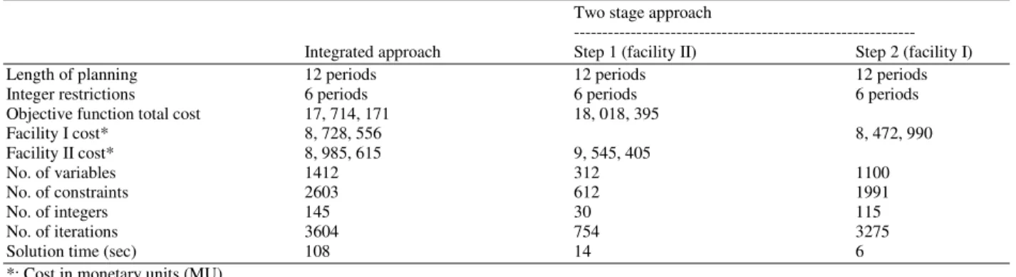
Table 1: Results of integrated and two stage approach
Two stage approach
---
Integrated approach Step 1 (facility II) Step 2 (facility I)
Length of planning 12 periods 12 periods 12 periods
Integer restrictions 6 periods 6 periods 6 periods
Objective function total cost 17, 714, 171 18, 018, 395
Facility I cost* 8, 728, 556 8, 472, 990
Facility II cost* 8, 985, 615 9, 545, 405
No. of variables 1412 312 1100
No. of constraints 2603 612 1991
No. of integers 145 30 115
No. of iterations 3604 754 3275
Solution time (sec) 108 14 6
*: Cost in monetary units (MU)
Sets of Constraints: Constraints 2, 3, 4, 5, 6, 7, 8, 12 and 13 and the nonegativity
Second step optimization (Plant I and transportation)
Minimize:
T L K
kt kt kt kt
kt kt kt t t kt
t 1 k 1 T L
t t t 1
(C X h I S r R o O )
C W
− ∧ ∧ ∧ ∧ ∧ ∧ ∧ ∧
= = −
=
+ + η + + +
(27)
Sets of Constraints: Constraints 9, 10, 11, 14, 15, 16, 17, 18, 19, 20, 21, 22, 23 and the nonegativity.
COMPUTATIONAL STUDY
The model's application is now illustrated using data taken from the specialty chemical firm. The case considered consists of five end products that are produced as a result of using eleven intermediate products and distilled water which can be described in the following manner: Product A is a lubricant agent that can be produced as a result of blending three intermediate products. The second product is B, a water soluble corrosion inhibitor that requires four intermediate products to be blended with distilled water (DW). The third end product C is a sulphuric lubricant that can be produced by blending six intermediate products. Product D, an anti foaming product that is manufactured as a result of blending two intermediate products and distilled water (DW). The fifth product E; a corrosion inhibitor requires three intermediate products to be manufactured. Figure 1 illustrates the end products, intermediate structure and solvents used in the study. In this study, the models were developed using OPL Studio version 3.6 and solved using CPLEX version 8. Models were executed with Pentium IV 2.80
End
A B C D E
DW 1 2 3 4 5 6 7 8 9 10 11
Intermediate and solvent
Fig. 1: End Products and intermediates product structure
GHz processor, while Microsoft Excel is used to export and import data and solution. Since the input data needed for our computational study is overwhelming, we have provided a small problem that consists of five end products that require eleven intermediates and single solvent to be produced as portrayed in Fig. 1.
RESULTS AND DISCUSSION
In Table 1, the integrated approach methodology has resulted in solving MIP problem that has 1412 variables, 2603 constraints and 145 integers. The computational time consumed to reach an optimal solution is 108 sec and model requires 3604 iterations to be solved. Examining the results for the two-step solution, the solution time to obtain an optimal solution has been reduced by about 24%. The integrated approach reduces objective function value by about 1.68%.
CONCLUSION
In this study we have developed a mixed integer linear programming problem that coordinates the production planning and transportation issues surrounding a specialty chemical plant. Our results indicate that the integrated approach to the problem is more beneficial in terms of cost savings. However, solving reasonably industrial size problem that include hundreds of products is not possible, since the computational time will increase exponentially as the number of integer variables increase. Consequently, the decision maker may not be able to obtain results in real time to be of any use for implementation purposes. One way around this problem is to restrict integer variables to certain time horizon as indicated earlier. It is worth noting that in case of the two-step approach, the integer restriction constitutes no problem in finding optimal solutions.
It is well known that MIP has an obvious weakness in solving reasonably industrial case. Currently the authors are involved in developing a genetic algorithm heuristic to provide a solution. However, the contribution of this research is providing MIP formulation that can provide solution for the small size problem which will be used in our future research to validate the performance of the heuristic avoiding the problem of testing one heuristic against another.
REFERENCES
1. Chandra, P. and M.L. Fisher, 1994. Coordination of Production and Distribution Planning. Eur. J. Operational Res., 72: 503-517.
2. Garcia, J.M. And S. Lozano, 2005. Production and Delivery Scheduling Problem with Time Windows. Comput. and Ind. Eng., 48: 733-742.
3. Haq, A.N., P. Vrat and A. Kanda, 1991. An Integrated Production-inventory-distribution Model for Manufacture of Urea: A Case. Int. J. Prod. Econ., 39: 39-49.
4. Jayaraman, V. and H. Pirkul, 2001. Planning and Coordination of Production and Distribution Facilities for Multiple Commodities. Eur. J. Operational Res., 36: 394-408.