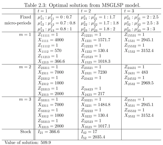
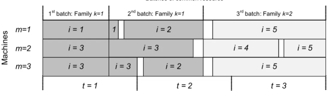
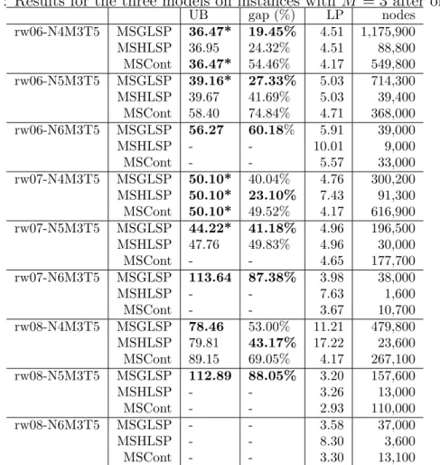
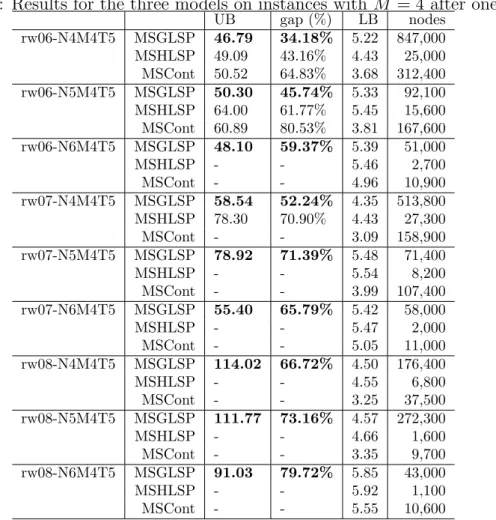
Otimização de processos na indústria têxtil: modelos e métodos de solução
Texto
Imagem


Documentos relacionados
didático e resolva as listas de exercícios (disponíveis no Classroom) referentes às obras de Carlos Drummond de Andrade, João Guimarães Rosa, Machado de Assis,
Ao Dr Oliver Duenisch pelos contatos feitos e orientação de língua estrangeira Ao Dr Agenor Maccari pela ajuda na viabilização da área do experimento de campo Ao Dr Rudi Arno
Neste trabalho o objetivo central foi a ampliação e adequação do procedimento e programa computacional baseado no programa comercial MSC.PATRAN, para a geração automática de modelos
Ousasse apontar algumas hipóteses para a solução desse problema público a partir do exposto dos autores usados como base para fundamentação teórica, da análise dos dados
i) A condutividade da matriz vítrea diminui com o aumento do tempo de tratamento térmico (Fig.. 241 pequena quantidade de cristais existentes na amostra já provoca um efeito
Peça de mão de alta rotação pneumática com sistema Push Button (botão para remoção de broca), podendo apresentar passagem dupla de ar e acoplamento para engate rápido
Este relatório relata as vivências experimentadas durante o estágio curricular, realizado na Farmácia S.Miguel, bem como todas as atividades/formações realizadas
Na hepatite B, as enzimas hepáticas têm valores menores tanto para quem toma quanto para os que não tomam café comparados ao vírus C, porém os dados foram estatisticamente
