Geographical externalities and the Pacifying Police Units Program in Rio de Janeiro

(1)

FUNDAC

¸ ˜

AO GET ´

ULIO VARGAS

ESCOLA de P ´

OS-GRADUAC

¸ ˜

AO em

ECONOMIA

Vinicius Rodrigues Pecanha

Geographical Externalities and The

Pacifying Police Unit Program in

Rio de Janeiro

(2)

Vinicius Rodrigues Pecanha

Geographical Externalities and The

Pacifying Police Unit Program in

Rio de Janeiro

Disserta¸c˜

ao para obten¸c˜

ao do grau de

mestre apresentada `

a Escola de P´

os-Gradua¸c˜

ao em Economia

´

Area de concentra¸c˜

ao:

Microecono-mia Aplicada

Orientador: Francisco J.M. Costa

(3)

Ficha catalográfica elaborada pela Biblioteca Mario Henrique Simonsen/FGV

Pecanha, Vinicius Rodrigues

Geographical externalities and the Pacifying Police Units in Rio de Janeiro / Vinicius Rodrigues Pecanha. - 2015.

47 f.

Dissertação (mestrado) - Fundação Getulio Vargas, Escola de Pós-Graduação em Economia.

Orientador: Francisco J. M. Costa. Inclui bibliografia.

1. Modelos econométricos. 2. Análise de séries temporais. 3. Análise espacial (Estatística). 4. Unidade de Polícia Pacificadora (Rio de Janeiro, RJ). I. Costa, Francisco Junqueiira Moreira da. II. Fundação Getulio Vargas. Escola de Pós- Graduação em Economia. III. Título.

(4)

(5)

Abstract

The paper quantifies the effects on violence and police activity of the Pacifying Police Unit program (UPP) in Rio de Janeiro and the possible geographical spillovers caused by this policy. This program consists of taking selected shantytowns controlled by criminals organizations back to the State. The strategy of the policy is to dislodge the criminals and then settle a permanent community-oriented police station in the slum. The installation of police units in these slums can generate geographical spillover effects to other regions of the State of Rio de Janeiro. We use the interrupted time series approach proposed by Gonzalez-Navarro (2013) to address effects of a police when there is contagion of the control group and we find that criminal outcomes decrease in areas of UPP and in areas near treated regions. Furthermore, we build a model which allows to perform counterfactuals of this policy and to estimate causal effects in other areas of the State of Rio de Janeiro outside the city.

(6)

1 Introduction

The structure of crime in Rio de Janeiro has some features that strengthen criminals gangs and hamper the combat against those. First, prison gangs1 _{control the retail drug}

market, what limits the punitive power of the State and makes these gangs more resilient (Lessing, 2013). Second, most of the drug gangs are located in the favelas, informal settlements incrusted in Rio’s mountains and hills. These groups usually control social and economic activities of the communities, impose their own laws and judge the conflicting cases (Dowdney, 2003). Due to the adverse geography of these places, police incursions are at disadvantage in clashes with criminals, what fortify the command of the traffickers over the slums (World Bank, 2012). This paper focus on the latter feature of the organization of crime in Rio de Janeiro and evaluates the impacts on violence and crime rates of a novel policy aimed to regain these territories controlled by drug gangs and restore the rule of law and the presence of the State in these communities.

The Pacifying Police Units program (UPP) was launched in 2008 and consists of taking selected shantytowns controlled by criminal organizations back to the State2

. The strategy of this policy is to dislodge the criminals and then settle a permanent community-oriented police station in the favela. The rise on the number of policemen allocated in these localities implies an increase in the law enforcement and the cost of doing drug business. As of December 2014, there are 9,000 policemen distributed in 38 police stations installed, covering 264 communities. Despite the relevance of accessing causal analyzes of this policy in violence and other social outcomes, there are few papers evaluating the impact of the program.

Butelli (2012) evaluates the impact of the pacification policy on short-term educa-tional outcomes. Neri (2011) and Frischtak and Mandel (2012) measure the effects of the reduction in crime rates due to the occupation of permanent police units in some fave-las on the prices of nearby residential property. More related to this paper, Ottoni and Ferraz (2013) and Cano (2012) study the reduction of violence and crime rates caused by the installation of these permanent police stations. Both papers utilize a differences-in-differences (DID) empirical strategy, defining the control group as the police stations that were not affected by program. The former paper also use a different control group, police stations in the interior of the State of Rio de Janeiro, in order to access possible crime displacement to untreated police stations in the city of Rio occurred after the beginning of the UPP program.

Dell (2014), Gonzalez-Navarro (2013) and Bronars and Lott (1998) show that crime displacement is a plausible outcome of a policy focused on a specific geographic unity. Therefore, the pacification policy may entail spatial externalities to non-pacified areas in

(8)

Rio. In situations in which the control group could be contaminated by the treatment, the assumption of ‘no interference of the control group’ (SUTVA) is violated and DID is not sound (Heckman, Lalonde and Smith, 1999 and Miguel and Kremer, 2004). This paper evaluates potential geographical spillovers to other areas in the city of Rio de Janeiro. We utilize interrupted time series strategy, discussed in Gonzalez-Navarro (2013) as a way to deal with interference problems in the control group and to verify spatial externalities within the city of Rio de Janeiro.3

We use official records data, monthly available from April 2003 to December 2014, provided by Instituto de Seguran¸ca P´ublica, research organization in public security of the Public Security Bureau of State of Rio de Janeiro. We have data at police station level for criminal outcomes and police activity. For criminal outcomes, we focus on homi-cides, street robbery, vehicle thefts and commercial burglary because we think that these represent the big picture of violence in a region. For police activity, we analyze drug and gun seizures, arrests and police killings because these variables are related with police actions against drug trafficking. We also have official data for the beginning of an UPP in a community and the police station responsible for that UPP.4

We find that, for police stations in which an UPP was installed, criminal outcomes decrease in a significant way. Thefts decrease almost 36percent and homicides fall 33 percent in areas treated by UPPs. Furthermore, police activity increase in this areas: drug seizures grow 124 percent, arrests 42 rise percent and police killings decreased 58 percent. For untreated police station located in the same Area Integrada de Seguranca Publica, a geographical concept of proximity, there is evidence for crime diffusion. Vehicle thefts, homicides, street robbery and thefts of commercial establishments decreased. We also find that as the number of police stations treated in the same AISP increase, the more crime diffusion occurs to untreated police stations in this same geographical area.5

Then, we intend to analyze geographical spillovers to areas outside the city of Rio de Janeiro. The potential crime displacement caused by the Pacifying Police Unit program hinders the definition of a valid control group. We propose an industrial organization’s entry model based on Seim (2006) and Orhun (2013), which give us, as an equilibrium outcome, the probability that a criminal agent enters in a given location and the number of criminals located in each area under the responsibility of a police station6_{. The main}

3_Let_Y

dtbe the potential outcomes in t, whered∈ {0,1}is the treatment status. Following Heckman,

Lalonde and Smith (2005) the assumption discussed above may be written as E[Y0t+1−Y0t|d = 1] =

E[Y0t+1−Y0t|d= 0]. With contagion of the control group, it is not reasonable to assume that this equality

holds. The trend of the control group depends on the treatment and it is not a good approximation as a counterfactual of the treatment group.

4

We understand a police station is treated when an UPP is installed in at least one of the communities under the responsibility of that police station

5_{In Appendix B, we discuss another geographical concept.}

(9)

advantage in using this approach is to perform counterfactual exercises altering the level of policemen or UPP treatment status in a police station and evaluating the expected number of criminals in each police station analyzed. For example, we can understand how police stations located outside the city of Rio de Janeiro would respond if all the police stations in the city of Rio were treated.

The paper proceeds as follow: the next section we discuss related literature in crime displacement or diffusion, section 3 details the data, section 4 shows the empirical strategy, section 5 describes the model and, at last, section 6 concludes the paper.

2 Related Literature

There are several models that address the question of crime displacement. Marceau (1997) discusses the effects of competition between jurisdictions in the eradication of crime. The key mechanism for his results is the crime displacement for adjacent localities caused by investments in crime deterrence technologies in a given jurisdiction. Deutsch, Hakim and Weinblatt (1987) relax the assumption that criminals have an expected net crime payoff that is decreasing in the distance between the site of the crime and their homes. This way, criminals consider only the expected revenue generated per crime and the probability of apprehension in a certain place in their optimization problems . They find that altering this probability for a given locality can increase the number of crimes committed in other districts.

Naranjo (2010) analyzes how domestic law enforcement policies by American local or state governments can affect other drug markets in United States. Matta and Andrade (2011) develop a linear city model based on location competition in crime between two regions in which individuals uniformly distributed between the cities can choose whether committing a crime in city A or B or work in the legal sector. They show that police intervention in high crime areas can displace criminals and increase the crime rate in the other locality. DeAngelo (2011) utilizes a circular city model and finds that a law enforcement technology can modify the spatial locations of criminal firms and the market share of these firms.

Helsley and Strange (1994) explore how expenditures on gating can divert criminals to other communities. The channel for displacement is the lower attractiveness of gated areas. They argue that gating always displace crime to other localities and may even increase the overall level of crime if employment opportunities are affected by this policy. Wheaton (2006) examines how a system of local law enforcement agencies in a metropoli-tan area impacts crime rates. Based on the equality of criminal’s utility in all regions and in an indirect utility function which is decreasing in the number of criminals in the area, he finds that increasing arrests in one town displaces criminals to all other towns.

(10)

protection divert crime. They build a model in which potential criminals are uniformly distributed between the victims, who may invest in private protection. In equilibrium, security expenditures are strategic complements when all potential criminals attempt theft and when the value of the property relative to potential criminal’s cost of switching between victims is high. Lee and Pinto (2009) examine a model with both private and public investment in crime prevention. The novel feature is that the public investment, besides displacing criminals to other localities, change incentives for investing in private protection for all the jurisdictions in the model. Therefore, the impact of public investment in a deterrence policy in criminals’ diversion is unclear and, under some specifications, the displacement effect of this policy can be reversed.

Although crime displacement caused by policies focused on deterrence may occur in equilibrium in the models analyze above, there is no robust evidence supporting this conjecture. On one hand, Bowers et al (2011) conduct a review analyzing the extent which deterrence policies cause crime displacement. Telep et al (2014) propose to answer the same question and survey the literature focusing on control interventions executed in medium and large geographic areas. Both papers find that crime displacement is not inevitable and, actually, diffusion benefits are as likely to occur as diversion. We should be cautious analyzing these results because, as Telep et al (2014) discuss, organized crime can face different incentives than isolated criminals to displace their criminal activities in response to policy intervention.

Draca, Machin and Witt (2010) estimate the causal impact of police on crime. They explore the increase in police units in some London boroughs in reaction to the terror attacks in London in 2005. It is argued that this a plausible exogenous variation in the cost of crime in these boroughs. They find that the intervention had clear direct effects, decreasing crime rates in the targeted boroughs. They also investigate the indirect effects for this intervention in other boroughs and did not find evidence for spatial criminal displacement.

Raudenbush and Verbitsky-Savitz (2012) estimate the impact of a community-policing program established in Chicago, designing an estimator that allows for the violation of the “no interference assumption” which avoids the problem of contagion of the control group. They define the potential outcome of a locality 𝑖 as a function of the treatment assignments to contiguous neighboring areas of 𝑖 and make the assumption that non-contiguous areas do not affect the potential outcome of 𝑖.7_{. They did not find evidence}

for crime displacement to areas near from the treatment regions.

On the other hand, there are papers that find evidence supporting crime displacement.

(11)

Gonzalez-Navarro (2013) investigates the impact of an auto-theft prevention technology (Lojack) installed in a specific type of car in some mexican states but not in others. Using an interrupted time series strategy, he finds that the introduction of this device had a deterrence effect on the vehicles participating the program and it was also responsible by geographical negative spillovers toward Lojack models in states not coverage by the Lojack policy.

Dell (2014) evaluates the causal impacts of crackdowns in violence and trafficking. Using a regression discontinuity design framework, she explores variations from close Mexican mayoral elections to isolate the effect of PAN, the party associated with the crackdowns, victories of the outcomes in violence and trafficking. She also builds a network model to discuss the spillover effects caused by this policy. Her results suggest that crackdowns caused lower crime rates in the localities governed by PAN and increased violence in other municipalities crossed by drug routes.

Jacob, Legfren and Moretti (2007) find evidence of intertemporal crime displacement, that is criminals may shift the time of their criminal activity in response to transitory changes in the price of crime. Bronars and Lott (1998) evaluates the spillover effects of a shall-issue conceal-weapons law in one state on neighboring areas. They find deleterious spillovers for property crimes, murder and robberies. Newlon (2001) also finds evidence for spatial displacement of crime.

As long as we know, this is the first paper that proposes an entry’s model to deal with potential violation of SUTVA in evaluating crime displacement. This specification allows us to deal with data restrictions. Although we do not have detailed data on price, costs and profits in these markets, we use criminals’ location choices to infer about relative profitability of the areas and to estimate the structural parameters. Furthermore, the model is empirically oriented, that is, it is designed to be structurally estimated, different than the models discussed above.

We also, considering the problem of contagion of control group, provided evidence for the open debate in crime displacement caused by a policy focused on a specific geographic area or ‘hot spot’ region.

3 Background and data

(12)

breaking the territorial domination of the drug gangs. The strategy of this policy is to dislodge the criminals and then settle a permanent community-oriented police station in the favela, not ending drug trafficking but allowing the State to operate in the favelas.

Then, the program was gradually expanded to other shantytowns. The Public Security Bureau uses two criteria to establish an UPP in a slum: (i) the favela is a poor community and (ii) is dominated by ostensibly armed criminal groups8_{. As of December 2014, there}

were 9,000 policemen distributed in 38 police stations installed, covering 264 communities. The rise on the number of policemen allocated in these localities implies an increase in the law enforcement and in the cost of doing drug business.

We use official records data from April 2003 to December 2014 at police station level monthly provided by ISP(Instituto de Seguran¸ca P´ublica). We have data at police station level for criminal outcomes and police activity. For criminal outcomes, we focus on homi-cides, street robbery, vehicle thefts and commercial burglary because we think that these represent the big picture of violence in a region. For police activity, we analyze drug and gun seizures, arrests and police killings.

Some police stations were created after the beginning of our database. To avoid missing observations, we added the criminal outcomes of these police stations to the police stations that were responsible for that area before the creation of the novel DP. For example, the 11 DP was created in December 2013 in Rocinha and we combined this police station with 15 DP, which was in charge of Rocinha before the establishment of the novel police station. As a result, we have observations of 130 police stations for 141 periods of time. Besides, there is no data for DP 54 during September 2005 and December 2005. We calculated the mean for the four months before and four months after and imputed the mean for the absent months.

We also utilize the dates of installations of Pacifying Police Units in the shantytowns and information about which police station each UPP is allocated, both available in UPP’s website9

. We understand there is a one-to-one relation between the installing of a UPP in a favela and the treatment in the police station in which this UPP is related. The definitions of Areas Integradas de Seguranca Publica (AISPs) and Zones of the city of Rio de Janeiro are supplied by ISP. Following the definition of Instituto de Seguranca P´ublica10_{, the statistical office of Secretary of Public Security, the geographical outline of}

each AISP was established from the area of operation of a military police battalion and the districts of civil police stations contained in the area of each battalion. There are 39 AISPs in the State of Rio de Janeiro and 17 only in the city of Rio.

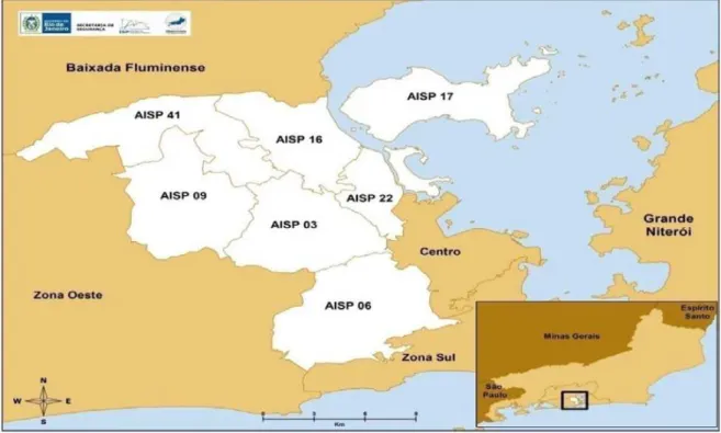
We also use the definition of Instituto de Seguranca P´ublica to define the Zones of the city of Rio de Janeiro. There four zones: (i) Zona Norte: AISPs 3 6 9 16 17 22 41; (ii)

8_{See http://www.upprj.com/index.php/faq.} 9_{http://www.upprj.com}

(13)

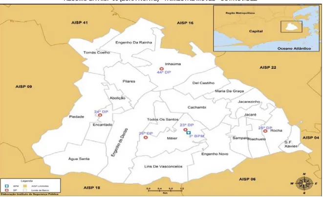
Zona Oeste: AISPs 14 18 27 31 40; (iii) Centro: AISPs 4 5; (iv) Zona Sul: AISPs 2 19 23. We took two figures from a report of Instituto de Seguran¸ca Publica to give an example of the previous definitions. Figure (1) shows AISPs that belong to North Zone of Rio and figure (2) shows the police stations in an AISP that belongs to the North Zone.

In order to facilitate the analysis of criminal outcomes, we defined two variables: (i) Violence lethality is given by the sum of homicides, police killings, injury followed by death and robbery with death and (ii) Thefts, defined as of roubo de rua by Instituto de Seguranca Publica as the sum of public transport robbery, mobile phone theft and robbery. These criminal outcomes are monthly reported by the Instituto de Seguran¸ca P´ublica.

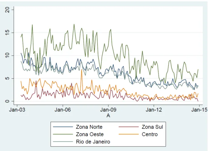
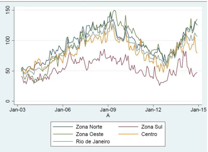
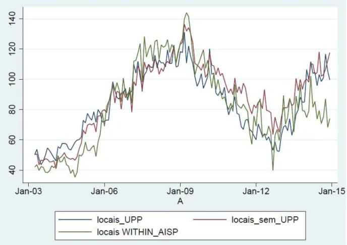
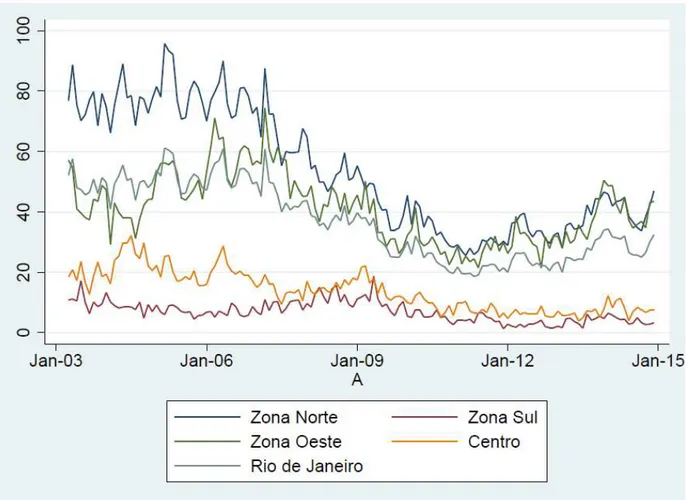
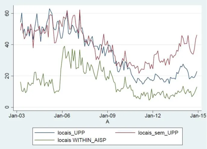
In table 1 we show the descriptive statistics. We can note that the variance is higher than the mean, one important feature of the estimation model that we will discuss above. Figures 4 to 9 show the evolution of absolute criminal outcomes in the zones and city of Rio de Janeiro and in police stations with UPP and without UPP in the city of Rio. We do not attempt to compare these numbers because we are not focusing on crime rates. Figures 4 and 5 show the evolution of violent mortality in zones of the city of Rio and in places with UPP and without UPP. We can see a steady decrease in this criminal outcome. Figures 6 and 7 display the evolution of thefts in the same areas discussed above. We find trend’s reversion after 2012 for almost all of the areas. Figures 8 and 9 discuss vehicle theft. For same areas, we can show a positive slope for the trend after 2012.

There are two concerns that one could raise about this data. First, since it is an official database, data can be manipulated11_{. For instance, after the beginning of the Pacifying}

program, information about criminal outcomes could be under-reported to gain political support for the program. Using this database, we cannot falsify this hypothesis. Second, after the installation of UPP in a favela, the probability of reporting a crime can change, that is, the likelihood of reporting a crime can increase. This possibility puts an upper bound to the estimators if they are negative. For example, if there is a negative correlation between thefts and introduction of UPPs and the premise of increasing likelihood of report is true, we expect that the estimator using the same likelihood of report as before the introduction of UPP should be lower. That is, even with people reporting more, the criminal outcome decreased.

4 Empirical strategy

The installation of UPPs in some shantytowns were not random. A shantytown must satisfy two criteria to be considered the instalation of an UPP in it: (i) it must be a poor

(14)

community and (ii) must be dominated by ostensibly armed drug gangs.12

Therefore, we must utilize a quasi-experiment approach to analyze the impact of UPPs in criminal out-comes and the possibility of geographical displacement. One of the necessary assumptions to conduct causal inference in this context is the Stable Unit Treatment Value Assump-tion (SUTVA)(Holland (1986)). The relevant component of this assumpAssump-tion for this paper is the “no interference” assumption, that is, the treatment status of an unit of analysis does not affect the outcomes of other units. The potential contagion of the control group violates this assumption, biasing the estimator what compromises the causal interpreta-tion of the program (Heckman, Lalonde and Smith (1999), Miguel and Kremer (2004), Bhattacharya et al(2013), Sobel (2006), Manski (2013)).

In the case of the Pacifying Police Unit program, the assumption above may not hold. Therefore, the pacification policy may entail spatial externalities to non-pacified areas in Rio. If these geographical externalities do occur, the difference-in-differences (DID) estimator will not precisely quantify the impact of the intervention on crime rates. If there is crime displacement to non-treated areas in the control group, the geographical externalities caused by the treatment introduce a negative bias in DID estimator and, therefore, underestimate the true impact. If crime diffusion occurs, the DID estimator would overestimate the true effect and introduce a lower-bound to the policy impact.

We choose an empirical strategy that can address this kind of problem. Following Gonzalez-Navarro (2013), we use an interrupted time series approach in which the coun-terfactual is given by the extrapolation of the trend estimated using pre-treatment obser-vations for the time period after the intervention. That is, without treatment an outcome would follow the same trend estimated with observations before the treatment. We eval-uate whether the treatment of some police stations altered the time series of criminal outcomes or police activity for police stations treated and for untreated police stations near from the treated. We discuss our distance metric before. The identifying assumption requires the introduction of UPPs in treated slums is not correlated with police activity or criminal outcomes before UPP.

We define treatment as the installation of a Pacifying Police Unit in a police station. We define a dummy UPP that is one for police stations and periods of time under the treatment of UPP and zero otherwise. In order to discuss geographical externalities in the city of Rio de Janeiro, we analyzed two possibilities.

First, we discuss the externalities generated by the introduction of UPP for police stations located near the favela treated. We use the definition of Areas Integradas de Se-guran¸ca Publica (AISP) to proxy this area of influence of treatment. An AISP encompass all the police stations under the responsibility of the same military police battalion. We

(15)

create the dummy WITHIN AISP that equals one for all untreated police stations located in a AISP after a police station of this area receives an UPP and zero for the treated police stations in this AISP. If a police station is treated, that is, the dummy UPP equals one, the dummy WITHIN AISP is zero, even if there is another treated police station in the same AISP. For example, in AISP 05 there are 4 police stations (DP 4, DP 5, DP 1 and DP 7). The first UPP in this AISP was installed in DP 4 in May 2010. The dummy UPP equals one for DP 4 from June 2010 until December 2014, WITHIN AISP remains zero for DP 4 throughout the whole period but this dummy equals one for all other police stations ( DP 5, DP 1 and DP 7) in AISP 05. In March 2011, the DP 7 received an UPP, therefore, the dummy UPP becomes one for DP 7 and the dummy WITHIN AISP goes to zero for DP 7. The value of WITHIN AISP to DP 5 and DP 1 remains one and to DP 4 remains zero.

The criminal outcomes such as homicides and thefts are count data, that is, they assume non-negative integer values and (some of them such as violence lethality) has significant mass on zero. To address this situation we follow Cameron and Trivedi (1998) and Gonzalez-Navarro (2013) and estimate the regressions using negative binomial models. We also control for police stations fixed effects and different linear trends for the police stations and clustered standard errors at police station level:

E[𝑌it] =𝑒𝑥𝑝{𝛼i+𝜆i𝑡+𝛽𝑈 𝑃 𝑃it} (1)

E[𝑌it] =𝑒𝑥𝑝{𝛼i+𝜆i𝑡+𝛾𝑊 𝐼𝑇 𝐻𝐼𝑁 𝐴𝐼𝑆𝑃it} (2)

where,𝑌it is some criminal outcome for police station 𝑖in period of time 𝑡, 𝛼i is the fixed

effect of police station𝑖and 𝜆i𝑡is the linear trend for𝐷𝑃i,𝑈 𝑃 𝑃it is a dummy that is one

if𝐷𝑃i has an UPP in period t and zero otherwise and WITHIN AISP is one if the police

station i is in the same AISP of other DP with UPP.

The coefficient on WITHIN AISP is our main coefficient of interest. If the coefficient is a positive value, means evidence of crime displacement and if it is negative means crime diffusion. If, the coefficient on UPP is negative, we can interpret that as a deterrence effect caused by the police. For the main results, I keep only the observations in the city of Rio.

Second, we allow for time fixed effects and estimate the same equations before with a term 𝜉t, which denotes the time fixed effects. Since the introduction of UPPs possible

causes geographical spillovers to other regions without UPP, this term captures part of the general equilibrium effects of UPP and its potential spillovers.

(16)

intensity of treatment as the percentage of police stations treated in a given AISP13

. Then, we allow two possible bands for the intensity of treatment: (i) band 1: if less or half of the police stations in a AISP were treated; (ii) band 2: more than half of the police stations in a AISP were treated. At last, we interacted this dummy variables with WITHIN AISP. We want to understand if untreated police stations exposed to more ‘treatment’ at AISP level react differently. We continue using the binomial negative model. Our regression in this case is: 14

E[𝑌it] = exp{𝛼i+𝜆i𝑡+𝛾1𝑊 𝐼𝑇 𝐻𝐼𝑁 𝐴𝐼𝑆𝑃 𝐵𝐴𝑁 𝐷1it+𝛾2𝑊 𝐼𝑇 𝐻𝐼𝑁 𝐴𝐼𝑆𝑃 𝐵𝐴𝑁 𝐷2it}

(3) The next section discuss the main results of the regressions analyzed above.

4.1 Results

We separate the regressions’ outcomes in two panels: Panel A shows the results for the regressions without time fixed effects and Panel B with time fixed effects. Then, we show two tables for the results: the first shows the results for criminal outcomes, such as homicides and thefts, and the second displays the results for policy activity, such as drug and gun seizures. Table 2 shows the results for criminal outcomes for police stations treated and polices stations untreated but located in AISPs that had at least one UPP installed and table 3 shows police activity for the same groups defined before. We also can verify the outcomes for police stations in which an UPP was installed. For both of them, we control for police stations fixed effects and allow linear time trends for each police station.

The dummy UPP represents the beginning of treatment in each police stations that had an UPP installed between 2009 and 2014 and the coefficients on this variable for vehicle thefts, violent mortality, homicides and thefts are negative and significant. This can be interpreted as a deterrence effect on the treated areas. For instance, violent mortality in places with UPP drops 33% and thefts 36%.15 _{Police activity also exhibit an}

improvement in police stations treated: drug seizures increase 124%, arrests increase 42% and police killings decrease 58%. This is interesting because not necessarily an increase in the number of policemen causes a grow in police activity. Rio’s police is characterized by corruption (Misse, 1997 and Lessing, 2013) and the policemen allocated in UPP areas could sell protection for drug traffickers instead of acting against them. The results shown in these table supports the idea that policemen in UPP areas are indeed combating drug trafficking.

13_{One, in this case, means that all the police stations of a given AISP were treated} 14_{We also estimate this equation with time fixed effects.}

(17)

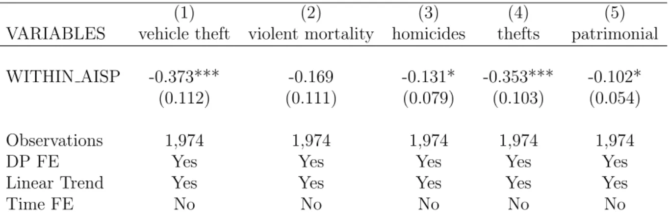
Tables 4 and 5 show evidence for criminal diffusion to police stations untreated near to police stations treated by an UPP, that is, for police stations in which the dummy WITHIN AISP equals one. This means that for untreated police stations located near from a police station with an UPP installed, there is a decrease in criminal outcomes. Vehicle thefts decreased 31%, homicides 12%, thefts 29% and thefts of commercial estab-lishments 9%.

However, police activity in police stations untreated doesn’t seen to change signifi-cantly. We have two hypothesis to explain this results: (i) criminals of these locations may have migrated to more distant areas, anticipating the installation of UPP in these areas and (ii) drug traffickers may have changed their behavior in order to avoid UPP presence in their favela. This could be merely an indirect deterrence effect of the police.

Tables 6 and 7 show the results for the intensity of treatment of AISPs. These tables show the more police stations are treated in an AISP, the smaller is the coefficient on WITHIN AISP. That is, the coefficient on WITHIN AISP BAND2 is smaller than the coefficient on WITHIN AISP BAND1. Both of these coefficients are negative for vehicle thefts, violent mortality, homicides and thefts. This suggests that the more intense the treatment the more crime diffusion occurs to police stations untreated but in the same AISP of at least one police station treated.

4.2 Placebo results

There are criminal offenses not related to drug trafficking which are not suppose to change differently in treated and untreated areas after the introduction of UPPs in some police stations such as culpable negligence16_{, larceny or extortion. We utilize the same framework}

as before to test this hypothesis. We control for police stations and allow linear and quadratic time trends for each police station. Table 8 shows the results for police stations treated and police stations untreated but in the same AISP of a treated DP. Both results corroborate the idea that types of crimes not related to physical violence didn’t change after the introduction of UPP in some shantytowns. The only exception in table 8 is extortion.

4.3 Robustness checks

First, to sustain our identifying assumption, we show that the levels of violence pre-UPP in locations where an UPP was installed, were not significantly different than other police stations in the city of Rio that didn’t have an UPP installed. The idea is that if there is no correlation between the installation of UPP and the criminal outcomes or police activity, we can understand the shift in time series of these variables as being caused by the policy. If there is correlation between the UPP and criminal outcomes, areas with

(18)

UPP could have an unobservable variable that is responsible both for the treatment and the outcomes in crime and police activity and we cannot assure that this unobservable variable remains constant throughout time. That is, in this situation, we could not use the trend estimated with observation pre-UPP as a counterfactual to the treatment.

We created a dummy for all police stations which have an UPP in December 2014 and utilize the negative binomial model to test the hypothesis that this places were more violent than other police stations in the city of Rio de Janeiro before the beginning of the UPP program in December 2009, using data between 2007 and 2008. Tables 9 and 10 show the results. We don’t reject the hypothesis that criminal outcomes of police stations with UPP during this period are not higher than other police stations in the city of Rio de Janeiro. That is, there is no evidence that the police stations treated between 2007 and 2008 were more violent than the other police stations in the city of Rio de Janeiro.

Second, we define a pseudo treatment in 2006. We restrict our database to April 2003 until December 2014 and define a new dummy UPP which turns one in January 2006 to all police stations treated in December 2014. We also define a new variable WITHIN AISP which turns one in January 2006 for all untreated police station in treated AISPs in December 2014. Tables 11 and 12 discuss the results for pseudo treatment for UPP and tables 13 and 14 for police stations with WITHIN AISP one in December 2014. As expected, we didn’t find evidence supporting a treatment effect for this pseudo treatment.

5 Model

Following Lessing (2008), we interpret drug dealers as firms that compete in the market of illegal drugs and seek to maximize their profits (earnings)17

. We allow firms to en-dogenously choose if they enter or not in the market and their geographic locations. We propose an incomplete information setting in which these choices are the outcomes. The assumption is that firms have private information about a location-specific idiosyncratic term. The main feature of the model is the competition effect that a firm suffers when it enters in a certain market, which allows use to explore the tradeoff between profitable areas and the magnitude of competition.

Agents choose whether enter in the criminal market and whether locate their activities. The agents’ payoff in the model depend on the characteristics of the demand and the actions of other agents, which determine the degree of competition in the place chosen to migrate to. Therefore, a game-theoretical approach will be necessary. Besides, we assume there is an idiosyncratic location-specific component in the agents’ payoff, which the researcher does not observe. To model this situation, we follow Seim (2006) and Orhun

(19)

(2013). This specification allows us to deal with data restrictions. Although we do not have detailed data on price, costs and profits in these markets, we use criminals’ location choices to infer about relative profitability of the areas and to estimate the structural parameters.

Agents compare expected static post-entry payoffs to make their entry and location choice. We explore the tradeoff between the profitability of the areas and the intensity of competition in these areas. The assumption is that competition impacts profits. Let Γ ={1,...,𝐿} be the a finite set of possible location options, which are mutually exclusive and exhaustive. 𝐸 is the number of potential entrants in the market and ∆ is the number of actual entrants.

An agent 𝑖 that chooses to enter in location 𝑙∈Γ, receives the following payoff:

𝑉il =Xl𝛽+𝑔(Λ∙l,n) +𝜒l+𝜖il (4)

where, Xl is a vector with observable variables that affect profitability of area 𝑙 such as

income, population, number of policemen, etc. and also contains a dummy associated with the presence of the program in that location .𝜖il is the location-specific idiosyncratic

term and𝑔(.) is a function that represents the impacts of competition on the agent located in𝑙. Λ is a ΓxΓ matrix in which the element𝜆ij reflects the effects that place𝑖imposes to

location 𝑗 due to competition.Thus, Λ∙l captures the competition’s interaction between

the other areas that belong to Γ with location𝑙 andnis a vector with the number of firms in each region of Γ. In this case of spatial competition, we can use the distance between two areas as a proxy for intensity of the competition. 𝜒l is a location specific component

that is known by the firms but not by the researcher similar to Orhun (2013).

An agent 𝑖 ∈ ∆ chooses to enter in location 𝑙 if and only if E[𝑉il] > E[𝑉ij] ∀𝑗 ∈

Γ, 𝑗 ̸=𝑙. The expectation operator reflects conjectures about the number of entrants in a location. We need to make some assumptions to make this problem tractable:

Assumption 1. The number of crimes in a region is a strictly increasing function in the number of criminals in that region.

Assumption 2. Players’ private information terms 𝜖1, ..., 𝜖E are independent and

identically drawn from a type-1 extreme value distribution.

Define distance bands d = {𝑑1_,𝑑2_,...,𝑑B_} _{around a focal area. Band} _𝑑b _{includes all}

areas 𝑗 such that𝑑b _≥_𝑑

jl> 𝑑b−1, where 𝑑jl is the physical distance between 𝑗 and 𝑙.

Assumption 3. The competition effect 𝑔(Λ∙l,n) = B

∑︀

b=1

𝛿b𝑛bl, where 𝑛bl is the number of

agents in band𝑏 around 𝑙.

(20)

use the data on the number of gun-related deaths in a location supplied by DATASUS. This kind of model has, as an equilibrium outcome, the probability that an agent enters in a given location and the number of firms located in each band. We understand UPP as an increase in the number of policemen a given location. Using this information as an observable covariate of equation (4), we can structurally estimate the parameters in a situation before UPP and, then, perform counterfactuals changing the level of policemen in a police station and analyzing the number of criminals expected in each band of the model. Manipulating the level of policemen in several locations could give us different treatment effects. For example, we can perform a situation in which all locations of the city of Rio have UPP and discuss the effects for the rest of the state or even try to estimate the optimal number of policemen in each location to minimize crime displacement.

Furthermore, if we have data on the different gangs that dominated one favela, an important feature of the drug’s market in Rio de Janeiro, we can follow Vitorino (2012) and relax Assumption 3. We can understand drug gangs as types and model this characteristic in a way that agents are able to observe their types before solving their entry and locational problem. This type is observable to players and to the researcher. We do not allow players to change their drug gang. With this specification we can relax assumption 3 and admit heterogenous competition effects depending on the drug gangs. Let Ω be the set of types. We can rewrite the assumption 3, for agent that belongs to gang 𝜔∈Ω as:

Assumption 3’ The competitive effect 𝑔ω_(Λ

∙l,n) =

∑︀

ω′∈Ω

B∑︀−1

d=1

𝛿ω′ d 𝑛

ω′

dl, where 𝑛 ω′

dl is the

number of agents in band𝑑 around 𝑙 which belong to gang 𝜔′

.

Neverthless, we are still collecting the necessary data to structurally estimate the parameters (𝛽, 𝛿). Then, we will implement the proposed exercises.

6 Conclusion

The Pacifying Police Unit program (UPP) was launched in 2008 and brought the State back in to more than 200 communities. Since the focus of these project is not to end with criminal activities but enable the entry of public goods in the slums, we have to question the possibility of criminal displacement to other areas of Rio. With this purpose, we estimated an interrupted time series model, similar to Gonzalez-Navarro (2013), and find that there is evidence for crime diffusion to areas near treated police stations .

Because of the possibility of contagion of the control group, it is more complicated to find geographical spillover to areas not in the city of Rio. To address this situation in which we can’t define a control group uncontaminated, we build a model based on Seim (2006) and Orhun (2013).

(21)

to control for some covariates such as population. We also can use Census’ variables to test if the installation of UPP in some communities were correlated with observable characteristics of these places, what is important to our identifying assumption. The interrupted time series framework discussed here can be applied with no restrictions to the georeferenced data. If we defined fixed bands in the city or even in the State of Rio de Janeiro, this can help understanding WITHIN AISP as a band in the model.

(22)

7 References

Amorim, C.1993. ”Comando Vermelho: a hist´oria do crime organizado” . Edi¸c˜oes Best Bolso.

Bhattacharya, D.; Dupas,P. and Kanaya,S. 2013.“Estimating the Impact of Means-tested Subsidies under Treatment Externalities with Application to Anti-Mallarial Bed-nets”. Working Paper.

Bresnahan, T. and Reiss, P. 1990. ”Entry in Monopoly Markets,” Review of Economic Studies, Wiley Blackwell, vol. 57(4), pages 531-53, October.

Bresnahan, T. and Reiss, P. 1991.”Entry and Competition in Concentrated Markets,” Journal of Political Economy, University of Chicago Press, vol. 99(5), pages 977-1009, October.

Bronars, S. and Lott, J. 1998. ”Criminal Deterrence, Geographic Spillovers, and the Right to Carry Concealed Handguns,” American Economic Review, American Economic Association, vol. 88(2), pages 475-79, May.

Bowers, K.; Johnson, S.; Guerette, R.; Summers, L; Poynton, S. 2011 ”Spatial dis-placement and diffusion of benefits among geographically focused policing initiatives: a meta-analytical review”. J EXP CRIMINOL , 7 (4) 347 - 374.

Butelli, P. 2012.”O impacto das UPPs sobre a performance escolar no Rio de Janeiro.” Masters’ thesis EPGE/FGV.

Cameron, C. A. and Trivedi, P. 2005. “Microeconometrics: Methods and Applica-tions”. Cambridge University Press.

Cano, I. 2012. ”Os donos do morro: uma avalia¸c˜ao explorat´oria do impacto das unidades de pol´ıcia pacificadores (UPPs) no Rio de Janeiro”. Working Paper.

da Matta, R. and Andrade, M., 2011. ”A model of local crime displacement,” Inter-national Review of Law and Economics, Elsevier, vol. 31(1), pages 30-36, March.

DeAngelo, G. 2012. ”Making space for crime: A spatial analysis of criminal competi-tion,” Regional Science and Urban Economics, Elsevier, vol. 42(1-2), pages 42-51.

Dell, M. 2014.“Trafficking Networks and the Mexican Drug War”. Working Paper Deutsch, J.; Hakim, S. and Weinblatt, J., 1987.”A micro model of the criminal’s loca-tion choice,” Journal of Urban Economics, Elsevier, vol. 22(2), pages 198-208, September. Draca, M.; Machin, S. and Witt, R. 2010. ”Crime Displacement and Police Inter-ventions: Evidence from London’s ’Operation Theseus’;,” NBER Chapters in: The Eco-nomics of Crime: Lessons for and from Latin America, pages 359-374 National Bureau of Economic Research, Inc.

Dowdney, L. 2003. ”Children of the drug trade: a case study of children in organised armed violence in Rio de Janeiro. Rio de Janeiro: 7Letras.

(23)

Gonzalez-Navarro,M. 2013. “Deterrence and Geographical Externalities in Auto-Theft”. American Economic Journal: Applied Economics, 5(4): 92-110.

Heckman,J.; Lalonde,R. and Smith,J. “Chapter 31 - The Economics and Econometrics of Active Labor Market Programs”’, In: Orley C. Ashenfelter and David Card, Editor(s), Handbook of Labor Economics, Elsevier, 1999, Volume 3, Part A, Pages 1865-2097, ISSN 1573-4463, ISBN 9780444501875, http://dx.doi.org/10.1016/S1573-4463(99)03012-6.

Helsley, R. and Strange, W. 1999. ”Gated Communities and the Economic Geography of Crime,” Journal of Urban Economics, Elsevier, vol. 46(1), pages 80-105, July.

Holland,P. 1986. ”Statistics and Causal Inference”. Journal of the American Statisti-cal Association Volume 81, Issue 396, 1986

Hui-Wen, K. and Png, I., 1994. ”Private security: Deterrent or diversion?,” Interna-tional Review of Law and Economics, Elsevier, vol. 14(1), pages 87-101, March.

Jacob, B.; Lefgren, L. and Moretti, E., 2005. ”The Dynamics of Criminal Behavior: Evidence from Weather Shocks,” Working Paper Series rwp05-003, Harvard University, John F. Kennedy School of Government.

Lee, K. and Pinto, S. M. 2009. ”Crime in a multi-jurisdictional model with private and public prevention”. Journal of Regional Science, 49: 977–996.

Lessing,B. 2008. “As Fac¸c˜oes Cariocas em Perspectiva Comparativa [Rio de Janeiro’s Drug Syndicates in Comparative Perspective].” CEBRAP Novos Estudos 80.

Lessing,B. 2013. “The Logic of Violence in Drug Wars: Cartel-State Conflict in Mex-ico, Brazil and Colombia.”. Working Paper.

Maddala, G. and Flores-Lagunes, A. 2001. “Qualitative response models” in B. Balt-agi, ed., A Companion to Theoretical Econometrics, Blackwell, Oxford.

Manski, C. 2001. “Daniel McFadden and the Econometric Analysis of Discrete Choice”. The Scandinavian Journal of Economics. Vol. 103, No. 2 (Jun., 2001), pp. 217-229

Manski, C. 2013. ”Identification of treatment response with social interactions,” Econometrics Journal, Royal Economic Society, vol. 16(1), pages S1-S23, 02.

Marceau,N. 1997. ”Competition in Crime Deterrence,” Canadian Journal of Eco-nomics, Canadian Economics Association, vol. 30(4), pages 844-54, November.

Miguel,E. and Kremer,M. 2004. “Worms: Identifying Impacts on Education and Health in the Presence of Treatment Externalities,” Econometrica, Econometric Society, vol. 72(1), pages 159-217, 01.

Misse, M. 1999. ”Malandros, Marginais e Vagabundos & a acumula¸c˜ao social da violˆencia no Rio de Janeiro”. IUPERJ doctoral thesis.

Naranjo, A. 2010. ”Spillover effects of domestic law enforcement policies,” Interna-tional Review of Law and Economics, Elsevier, vol. 30(3), pages 265-275, September.

Neri,M. 2011. ”UPP2 e a Economia da Rocinha e do Alem˜ao: do Choque de Ordem ao de Progresso””. Working Paper.

(24)

a municipal level analysis”. Working Paper.

Orhun, A. 2013.”Spatial differentiation in the supermarket industry: The role of com-mon information,” Quantitative Marketing and Economics, Springer, vol. 11(1), pages 3-37, March.

Ottoni,B. and Ferraz, C. 2013.“State Presence and Urban Violence: Evidence from the Pacification of Rio’s Favelas”. Working Paper.

Savitz-Verbitsky, N. and Raudenbush, S.W. (2012). Causal inference under interfer-ence in spatial settings: A case study evaluating community policing program in Chicago. Epidemiologic Methods. Vol. 1, Issue 1, pp 107 – 130. (Online) 2161-962X, DOI: 10.1515/2161-962X.1020

Seim, K.2006. An empirical model of firm entry with endogenous producttype choices. RAND Journal of Economics, RAND Corporation, vol. 37(3), pages 619-640, 09.

Sobel, M.E. (2006) What do randomized studies of housing mobility demonstrate?:Causal inference in the face of interference. Journal of the American Statistical Association, 101:1398-1407.

Telep, C. , Weisburd, D. , Teichman, D. , Gill, C. E. and Vitter, Z. 2014.Displace-ment of Crime and Diffusion of Crime Control Benefits in Large-Scale Geographic Areas: A Systematic Review. Paper presented at the annual meeting of the ASC Annual Meeting,

Washington Hilton, Washington, DC. 2014-11-25 from http:citation.allacademic.com/meta/p515538i𝑛𝑑𝑒𝑥.ℎ𝑡𝑚𝑙

Vitorino, M. 2012. Empirical Entry Games with Complementarities: An Application to the Shopping Center Industry. Journal of Marketing Research, 2012, 49(2), 175-191.

Wheaton,W. 2006. Metropolitan fragmentation, law enforcement effort and urban crime. Journal of Urban Economics, Volume 60, Issue 1, July 2006, Pages 1-14, ISSN 0094-1190, http://dx.doi.org/10.1016/j.jue.2006.01.005.

(25)

8 Appendix A

In this part, I discuss the bias caused by contagion of the treatment group when using the differences-in-differences estimator. Let 𝑌dt be the potential outcomes in t, where

𝑑∈ {0,1} is the treatment status. The assumption of DD estimator is: E[𝑌0t+1−𝑌0t|𝑑=

1] =E[𝑌0t+1−𝑌0t|𝑑= 0]. Crime displacement can violate this assumption. Let ℒ be the

set of slums in Rio and𝑇 ⊂ ℒ the subset of slums treated by UPP. T actual model is:

𝑌it=𝛾i+𝜆t+𝛿1𝐷it+𝛿2(1−𝐷it)𝑔i(𝑇, 𝑛T) +𝜖it

where𝑔i(𝑇, 𝑛T) maps the migration of criminals to region𝑖due to the pacification of their

favelas. For simplicity, in 𝑡= 0, 𝑇 = 0 and𝑔i(0, 𝑛T) = 0

If we do not consider crime displacement, we will estimate 𝑌it = 𝛾i +𝜆t+𝛿𝐷it+ ˜𝜖it

where, E[˜𝜖i1|𝐷i1 = 0] ̸= 0. Let ∆ = E[𝛿2(1−𝐷it)𝑔i(𝑇, 𝑛T)|𝐷i1 = 0, 𝑡 = 1]. If crime

displacement occurs, ∆≥0. If crime diffusion occurs, ∆ ≤0. Population DD:

{E[𝑌it|𝐷i1 = 1, 𝑡= 1]−E[𝑌i0|𝐷i1 = 1, 𝑡= 0]}

−{E[𝑌i1|𝐷i1 = 0, 𝑡= 1]−E[𝑌i0|𝐷i1 = 0, 𝑡= 0]}

=𝛿−∆

9 Appendix B

We define another concept of proximity for untreated police stations in a AISP where none of the police stations allocated in this Area Integrada were treated, but in a zone with at least one treated police station. This concept allows us to discuss geographical externalities to a larger area. Besides, the zones of the city of Rio de Janeiro can capture preferred channels of migration because the slums in a zone might be more similar than other areas, they can share the same drug market or geographical proximity might enhance social capital among criminals in these locations, which can increase the probability that a criminal in a treated favela migrate to a slum in the same zone. The hypothesis being tested is if there is evidence for crime displacement to untreated areas more distant from a treated police station. We find that there is also a reduction in criminal outcomes.

We define other dummy, WITHIN ZONE, to capture the effect of UPP in police stations that were untreated but were in the same zone of a police station treated. This dummy turns one when there is an installing of UPP in another AISP of the same of of this police station.

(26)

(27)

10 Figures and Tables

Figure 1: AISPs in North Zone

(28)

Figure 2: Police stations in AISP 3 (North Zone)

(29)

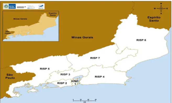
Figure 3: RISPs in the State of Rio de Janeiro

Fonte: Instituto de Seguranca Publica

Table 1: Summary statistics

Variable Mean Std. Dev.

homicides 4.10 5.16 vehicle theft 36.79 34.88 thefts 85.55 50.02 commercial burglary 5.86 4.30 violence lethality 5.48 6.39 drug seizures 10.69 14.78 gun seizures 8.46 9.77 police killings 1.15 2.10 arrests 17.84 18.14 culpable homicides 1.56 1.93 larceny 30.93 28.85 extortion 1.95 2.35

(30)

Figure 4: Evolution of violent mortality in the zones of the city of Rio de Janeiro

(31)

Figure 5: Evolution of violent mortality in police stations with UPP, without UPP and WITHIN AISP

(32)

Figure 6: Evolution of thefts in the zones of the city of Rio de Janeiro

(33)

Figure 7: Evolution of thefts in police stations with UPP, without UPP and WITHIN AISP

(34)

Figure 8: Evolution of vehicle thefts in the zones of the city of Rio de Janeiro

(35)

Figure 9: Evolution of vehicle thefts in police stations with UPP, without UPP and WITHIN AISP

(36)

Table 2: Effects of UPP in criminal outcomes:

Panel A: Without Time FE

(1) (2) (3) (4) (5)

VARIABLES vehicle theft violent mortality homicidies thefts patrimonial

UPP -0.227 -0.410*** -0.291*** -0.456*** 0.171* (0.154) (0.102) (0.090) (0.075) (0.094)

Observations 3,243 3,243 3,243 3,243 3,243

DP FE Yes Yes Yes Yes Yes

Linear Trend Yes Yes Yes Yes Yes

Time FE No No No No No

Panel B: With Time FE

(1) (2) (3) (4) (5)

VARIABLES vehicle theft violent mortality homicides thefts patrimonial

UPP -0.147 -0.200* -0.185* -0.009 -0.043 (0.099) (0.112) (0.099) (0.043) (0.062)

Observations 3,243 3,243 3,243 3,243 3,243

Time FE Yes Yes Yes Yes Yes

Note: _{We included police stations fixed effects, a linear trend to each police station and clustered}

(37)

Table 3: Effects of UPP in police activity:

Panel A: Without Time FE

(1) (2) (3) (4)

VARIABLES drug seizures gun seizures police killings arrests

UPP 0.809*** -0.110 -0.885*** 0.355** (0.131) (0.111) (0.233) (0.140)

Observations 3,243 3,243 3,243 3,243

DP FE Yes Yes Yes Yes

Linear Trend Yes Yes Yes Yes

Time FE No No No No

Panel B: With Time FE

(1) (2) (3) (4)

UPP 0.380*** -0.110 -0.239 0.188 (0.110) (0.111) (0.245) (0.164)

Observations 3,243 3,243 3,243 3,243

Time FE Yes Yes Yes Yes

(38)

Table 4: Geographical externalities to untreated police stations located in the same AISP

Panel A: Without time fixed effects

(1) (2) (3) (4) (5)

WITHIN AISP -0.373*** -0.169 -0.131* -0.353*** -0.102* (0.112) (0.111) (0.079) (0.103) (0.054)

Observations 1,974 1,974 1,974 1,974 1,974

Panel B: With time fixed effects:

(1) (2) (3) (4) (5)

WITHIN AISP -0.064 0.016 -0.048 -0.079 0.010 (0.120) (0.114) (0.118) (0.067) (0.066)

Observations 1,974 1,974 1,974 1,974 1,974

Note: _{We included police stations fixed effects, a linear trend to each police station and}

clus-tered standard errors at police station level. We utilize equation E[Yit] = exp{αi +λit+

(39)

Table 5: Geographical externalities to untreated police stations located in the same AISP

(1) (2) (3) (4)

WITHIN AISP -0.395*** -0.134 -0.243 -0.085 (0.074) (0.147) (0.237) (0.187)

Observations 1,974 1,974 1,974 1,974

Time FE No No No No

(1) (2) (3) (4)

WITHIN AISP 0.005 0.0736 0.0640 -0.181 (0.120) (0.116) (0.172) (0.135)

Observations 1,974 1,974 1,974 1,974

(40)

Table 6: Treatment Intensity for AISPs:

(1) (2) (3) (4) (5)

WITHIN AISP BAND1 -0.367*** -0.134 -0.102 -0.332*** -0.108* (0.106) (0.094) (0.068) (0.091) (0.057) WITHIN AISP BAND2 -0.418** -0.525 -0.469 -0.516* -0.052

(0.213) (0.411) (0.338) (0.293) (0.135)

Observations 1,974 1,974 1,974 1,974 1,974

(1) (2) (3) (4) (5)

WITHIN AISP BAND1 -0.019 0.085 0.017 -0.044 0.036 (0.098) (0.087) (0.106) (0.053) (0.063) WITHIN AISP BAND2 -0.255 -0.420 -0.483 -0.262 -0.120

(0.316) (0.419) (0.348) (0.205) (0.238)

Observations 1,974 1,974 1,974 1,974 1,974

clus-tered standard errors at police station level. We utilize equation _E[Yit] = exp{αi +λit+

γ1W IT HIN AISP BAN D1it +γ2W IT HIN AISP BAN D2it}. WITHIN AISP BAND1 is

(41)

Table 7: Treatment Intensity for AISPs:

(1) (2) (3) (4)

WITHIN AISP BAND1 -0.409*** -0.110 -0.205 -0.011 (0.079) (0.151) (0.219) (0.184) WITHIN AISP BAND2 -0.275 -0.326 -0.581 -0.926***

(0.187) (0.237) (0.637) (0.180)

Observations 1,974 1,974 1,974 1,974

Time FE No No No No

(1) (2) (3) (4)

WITHIN AISP BAND1 0.052 0.141 0.110 -0.084 (0.125) (0.0981) (0.150) (0.156) WITHIN AISP BAND2 -0.252 -0.299 -0.209 -1.023***

(0.221) (0.370) (0.708) (0.198)

Observations 1,974 1,974 1,974 1,974

γ1W IT HIN AISP BAN D1it +γ2W IT HIN AISP BAN D2it}. WITHIN AISP BAND1 is

(42)

41

(1) (2) (3) (4) (5) (6) culpable negligency larceny extortion culpable negligency larceny extortion

UPP -0.015 0.048 0.221** -0.081 0.006 0.204** (0.066) (0.069) (0.112) (0.082) (0.062) (0.088) WITHIN AISP 0.107* 0.075 0.045 0.014 -0.037 0.039

(0.064) (0.060) (0.122) (0.067) (0.057) (0.103)

Observations 4,743 5,139 5,139 4,743 5,139 5,139 DP FE Yes Yes Yes Yes Yes Yes Linear Trend No No No Yes Yes Yes Quadratic Trend Yes Yes Yes No No No

Note: _{We included police stations fixed effects, a linear trend to each police station and clustered standard errors at police station}

(43)

Table 9: UPP stations between January 2007 and December 2008

(1) (2) (3) (4) (5)

locais UPP -0.254 -0.082 -0.222 0.144 -0.499 (0.438) (0.332) (0.374) (0.157) (0.433)

Observations 936 936 936 936 936

DP FE No No No No No

Notes: _{The dummy locais UPP equals one for all police stations that have an UPP in December}

2014. We restrict our observations between January 2007 and December 2008 and control for police station fixed effects and for a linear trend for each police stations. We clustered standard errors at the police station level.

Table 10: Table: UPP stations between January 2007 and December 2008

(1) (2) (3) (4)

locais UPP 0.137 0.709* -0.111 0.113 (0.669) (0.416) (0.672) (0.446)

Observations 936 936 936 936

DP FE No No No No

Notes: _{The dummy locais UPP equals one for all police stations that have an UPP in December}

2014. We restrict our observations between January 2007 and December 2008 and control for police station fixed effects and for a linear trend for each police stations. We clustered standard errors at the police station level.

Table 11: Pseudo treatment in 2006 for police stations treated in december 2014:

(1) (2) (3) (4) (5)

UPP 0.026 0.051 0.059 0.075* -0.135 (0.058) (0.067) (0.056) (0.041) (0.085)

Observations 1,587 1,587 1,587 1,587 1,587

(44)

Table 12: Pseudo treatment in 2006 for police stations treated in december 2014:

(1) (2) (3) (4)

UPP 0.198* -0.0217 0.0195 0.008 (0.114) (0.0482) (0.144) (0.059)

Observations 1,587 1,587 1,587 1,587

Time FE No No No No

standard errors at police station level. We restrict our database to April 2003 until December 2014 and define a dummy UPP which turns one in January 2006 to all police stations treated in December 2014.

Table 13: Pseudo treatment in 2006 for police stations untreated located in treated AISP in december 2014:

(1) (2) (3) (4) (5)

WITHIN AISP 1.138 0.599 0.471 0.768 0.220 (0.791) (0.869) (0.721) (0.768) (0.274)

Observations 276 276 276 276 276

(45)

Table 14: Pseudo treatment in 2006 for police stations untreated located in treated AISP in december 2014:

(1) (2) (3) (4)

WITHIN AISP 0.773 0.464 1.003 0.345 (0.912) (0.837) (1.813) (0.639)

Observations 276 276 276 276

Time FE No No No No

standard errors at police station level. We restrict our database to April 2003 until December 2014 and define a dummy WITHIN AISP which turns one in January 2006 to all police stations untreated but in treated AISP in December 2014.

Table 15: Geographical externalities to police stations located in the same AISP and in the some Zone:

(1) (2) (3) (4) (5)

vehicle theft violent mortality homicidies thefts patrimonial

UPP -0.484*** -0.578*** -0.416*** -0.726*** 0.217* (0.149) (0.101) (0.094) (0.078) (0.111) WITHIN AISP -0.632*** -0.398*** -0.298*** -0.641*** -0.003

(0.141) (0.110) (0.082) (0.097) (0.070) WITHIN ZONE1 -0.255*** -0.287*** -0.197*** -0.336*** 0.159***

(0.071) (0.081) (0.067) (0.062) (0.056)

Observations 5,499 5,499 5,499 5,499 5,499

standard errors at police station level. We utilize equationE[Yit] =exp{αi+λit+β1U P Pit+

β2W IT HIN AISPit+β3W IT HIN ZON E1it}. WITHIN AISP is dummy that turn one if a

(46)

Table 16: Geographical externalities to police stations located in the same AISP and in the some Zone:

(1) (2) (3) (4)

drug seizures gun seizures police killings arrests

UPP 0.862*** -0.193 -1.218*** 0.444*** (0.157) (0.119) (0.221) (0.161) WITHIN AISP 0.014 -0.214 -0.728*** 0.108

(0.100) (0.149) (0.248) (0.197) WITHIN ZONE1 0.147 -0.0713 -0.642*** 0.237

(0.096) (0.0918) (0.149) (0.145)

Observations 5,499 5,499 5,499 5,499

standard errors at police station level. We utilize equationE[Yit] =exp{αi+λit+β1U P Pit+

β2W IT HIN AISPit+β3W IT HIN ZON E1it}. WITHIN AISP is dummy that turn one if a

Geographical externalities and the Pacifying Police Units Program in Rio de Janeiro

FUNDAC

¸ ˜

AO GET ´

ULIO VARGAS

ESCOLA de P ´

OS-GRADUAC

¸ ˜

AO em

ECONOMIA

Vinicius Rodrigues Pecanha

Geographical Externalities and The

Pacifying Police Unit Program in

Rio de Janeiro

Vinicius Rodrigues Pecanha

Geographical Externalities and The

Pacifying Police Unit Program in

Rio de Janeiro

Disserta¸c˜

ao para obten¸c˜

ao do grau de

mestre apresentada `

a Escola de P´

os-Gradua¸c˜

ao em Economia

´

Area de concentra¸c˜

ao:

Microecono-mia Aplicada

Orientador: Francisco J.M. Costa

Abstract

Contents

1

Introduction

2

Related Literature

3

Background and data

4

Empirical strategy

4.1

Results

4.2

Placebo results

4.3

Robustness checks

5

Model

6

Conclusion

7

References

8

Appendix A

9

Appendix B

10

Figures and Tables