MODELAGEM E AN ´
ALISE DE
CONECTIVIDADE EM REDES SEM FIOS
MARCELO GABRIEL ALMIRON
MODELAGEM E AN ´
ALISE DE
CONECTIVIDADE EM REDES SEM FIOS
OBSTRU´
IDAS
Tese apresentada ao Programa de P´os--Gradua¸c˜ao em Ciˆencia da Computa¸c˜ao do Instituto de Ciˆencias Exatas da Universi-dade Federal de Minas Gerais como req-uisito parcial para a obten¸c˜ao do grau de Doutor em Ciˆencia da Computa¸c˜ao.
Orientadora: Olga Nikolaevna Goussevskaia
Coorientadores: Antonio A.F. Loureiro &
Alejandro C. Frery
MARCELO GABRIEL ALMIRON
MODELING AND CONNECTIVITY ANALYSIS
IN OBSTRUCTED WIRELESS NETWORKS
Thesis presented to the Graduate Program in Computer Science of the Federal Univer-sity of Minas Gerais in partial fulfillment of the requirements for the degree of Doctor in Computer Science.
Advisor: Olga Nikolaevna Goussevskaia
Co-Advisors: Antonio A.F. Loureiro & Alejandro C. Frery
c
2014, Marcelo Gabriel Almiron. Todos os direitos reservados.
Ficha catalogr´afica elaborada pela Biblioteca do ICEx - UFMG
Almiron, Marcelo Gabriel
A449m Modelagem e An´alise de Conectividade em Redes Sem Fios Obstru´ıdas / Marcelo Gabriel Almiron. — Belo Horizonte, MG, 2014
xx, 73 f. : il. ; 29cm
Tese (Doutorado) — Universidade Federal de Minas Gerais - Departamento de Ciˆencia da Computa¸c˜ao
Orientadora: Olga Nikolaevna Goussevskaia Coorientadores: Antonio Alfredo Ferreira Loureiro
Alejandro C´esar Frery Orgambide 1. Computa¸c˜ao Teses. 2. Redes de computadores -Teses. 3. Sistemas de comunica¸c˜ao sem fios - -Teses. I. Orientador. II. Coorientador. III. T´ıtulo.
A mis padres, Stella Maris y Pedro Jos´e.
Acknowledgments
First, I thank my parents, Stella Maris and Pedro Jos´e, my sisters, Marit´e and Laura, and my brother, Jos´e. They gave me all means to achieve what I dreamed about in my life, and I will always be thankful.
Special thanks to my mentors, Profa. Olga N. Goussevskaia, Prof. Antonio A.F. Loureiro, Prof. Alejandro C. Frery and Prof. Jos´e Rolim. I was very fortunate for being surrounded by excellent people and researchers with plurality of thinking and areas of expertise.
I thank my friends from UFMG: Anderson, Anna, Alyson, Bruno (Lopes and Silva), Celso, C´esar, Christian, Clayson, Daniel (Galinkin and Guidoni), Eduardo, Evellyn, Felipe, Fernanda, Fernando, Fl´avio, Guilherme, Heitor, Ilo, Izabela, John, K´assio, Laura, Leandro, Let´ıcia, Lorena, Luciana, Max, Marcos, Pedro (Silva and Stancioli), Rafael (Colares, Santin and Siqueira), Rodolfo, Thiago, Tiago, Vin´ıcius and Zilton. It was and will continue being a wonderful group!
My thanks also to Aubin, Cristina, Eugenio, Hakob, Kasun, Konstantinos, Mar-ios, Orestis, Pierre and Tigran, for their friendship and shared moments during my stay in University of Geneva.
Finally, my very special thanks to Kl´arka for supporting me in the last and more critical moment making me feel her love at every second, on occasions, with the Atlantic Ocean between us.
Resumo
Propriedades de conectividade de redes sem fio em espa¸cos abertos normalmente s˜ao modeladas utilizando grafos aleat´orios geom´etricos, e j´a foram analisadas em profun-didade em diferentes estudos. Esses cen´arios, no entanto, n˜ao representam, no geral, situa¸c˜oes reais encontradas na pr´atica, tais como ambientes urbanos ou espa¸cos fecha-dos, que s˜ao profundamente afetados por obst´aculos. Como alternativa, propomos um modelo para redes sem fio ad hoc obstru´ıdas, formadas por um conjunto de n´os posicionados de maneira aleat´oria numa grade, onde todos os n´os compartilham um mesmo raio de transmiss˜ao. Para o posicionamento dos n´os no ambiente, todos os seg-mentos s˜ao considerados como sendo unidimensionais, mas para fins de comunica¸c˜ao, adicionamos um parˆametro ǫ para modelar a largura dos segmentos. N´os mostramos como o modelo resultante pode ser utilizado para estudar as propriedades destas redes de comunica¸c˜ao de maneira anal´ıtica e para simular uma variedade de topologias de rede com o intuito de avaliar o desempenho de protocolos de comunica¸c˜ao nos cen´arios acima mencionados.
Para calcular a probabilidade de conectividade em interse¸c˜oes de segmentos (Pr(Icon)), propomos trˆes modelos geom´etricos diferentes: os modelos Max-Norm,
Line-of-Sight (LoS) e Triangular. Mostramos a dificuldade de computo de Pr(Icon) sob
o modelo LoS, e calculamos limites inferiores para Pr(Icon) sob os modelos Max-Norm
e Triangular, com o respectivo limite superior no erro de aproxima¸c˜ao.
Adicionalmente, introduzimos uma abstra¸c˜ao na grade e aplicamos a teoria de percola¸c˜ao para calcular a raio m´ınimo de transmiss˜ao que gera conectividade, no gr´afo de comunica¸c˜oes, com alta probabilidade. Esta solu¸c˜ao exige um m´ınimo de visibilidade nos cruzamentos dentre segmentos, e esta visibilidade depende do parˆametro ǫ. Com isto, calculamos a visibilidade m´ınima exigida para ter conectividade quando utilizamos o raio de transmiss˜ao m´ınimo derivado. Este raio de transmiss˜ao especifico ´e con-hecido como o alcance de transmiss˜ao m´ınimo para conectividade (em inglˆes, Critical Transmission Range (CTR)), e provamos que o CTR para conectividade derivado n˜ao depende do modelo geom´etrico em cruzamentos. Fizemos um estudo da escalabilidade
de redes obstru´ıdas dentro do modelo proposto e desenvolvemos m´etodos anal´ıticos para determinar se h´a possibilidade de obter conectividade com alta probabilidade em topologias homogˆeneas de rede para determinadas combina¸c˜oes de caracter´ısticas, tais como largura dos segmentos, tamanho da grade e limite tecnol´ogico do raio m´aximo de transmiss˜ao.
Abstract
Connectivity properties of wireless networks in open space are typically modeled us-ing geometric random graphs and have been analyzed in depth in different studies. Such scenarios, however, do not often represent situations encountered in practice, like urban environments or indoor spaces, which are deeply affected by obstacles. As an alternative, we propose a model for obstructed wireless ad hoc networks consist-ing of a set of nodes deployed at random in a grid, all of them sharconsist-ing a common transmission range. For positioning the nodes in the field, all segments are consid-ered as being one-dimensional, but for communication purposes, we add a parameter
ǫ to model the segments’ width. We show how the resulting model can be used to study properties of such communication networks analytically and to simulate a va-riety of network topologies for performance evaluation of communication protocols in the aforementioned scenarios.
In order to compute the probability of connectivity at segments’ intersections (Pr(Icon)), we propose three different geometric models, namely, the Max-Norm, LoS
and Triangular models. We show the difficulty of computing Pr(Icon) under the LoS,
and we compute tight lower bounds for Pr(Icon) under the Max-Norm and Triangular
models, with the respective upper bound of the approximation error.
Additionally, we introduce an abstraction on the grid and apply percolation the-ory to compute the minimum transmission range that generates communication graphs that are connected with high probability (w.h.p.). The solution requires a minimal visibility at intersections, depending on the parameter ǫ. We compute the minimal visibility required to have connectivity using the derived minimum transmission range. This particular transmission range is known as the CTR for connectivity, and we prove that the derived CTR for connectivity does not depends on the geometrical model at intersections. We performed a study of the scalability of obstructed networks within the proposed model and developed analytical methods to determine the possibility of obtaining connectivity w.h.p. in homogeneous topologies for specific combinations of characteristics, e.g. segments’ width, grid size and the maximum transmission range.
List of Figures
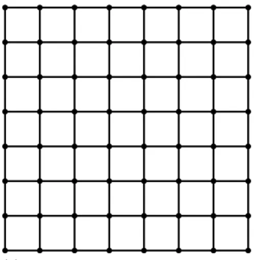
1.1 Line-of-sight network model of Frieze et al., with p= 0.45 and ω= 2, on a
grid of 8×8. . . 2
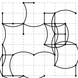
1.2 An instance of an obstructed wireless network with densityµ= 5 deployed in an 8×8 scenario and using transmission range r = 0.65. Gray areas represent the obstacles; regions in the space with infinite path loss. The communication criterion corresponds to our LoS model. . . 3
1.3 Modeling obstructed wireless networks so as to derive the CTR for Connec-tivity. . . 6
2.1 The geometrical layer: an urban obstructed environment with nodes de-ployed uniformly at random. The environment is defined by the granularity g = 4 and the segments’ width parameter ǫ. . . 11
2.2 Determining the communication links present at street intersections. The gray region represents the coverage of node u. . . 13
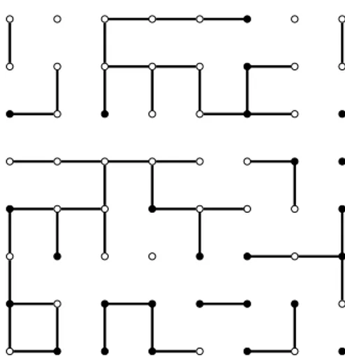
2.3 Intances of the random grid G8, with V = {1,2, . . . ,8}2, while using two different values for the probability of edges in a bond percolation model. . 15
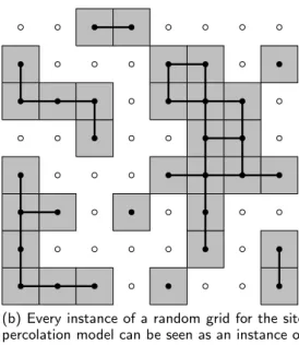
2.4 An instance of a random grid for the site percolation model withg = 8, and the relationship with an instance of a bond percolation model. . . 16
2.5 An extension of the bond percolation instance of Figure 2.3b with site prob-abilityps =pb = 0.45. . . 17
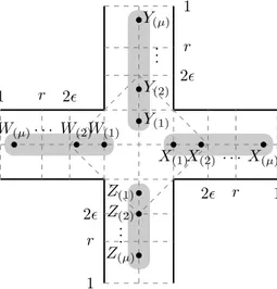
3.1 Reference scenario for connectivity at intersections . . . 20
3.2 Intersection Graph . . . 21
3.3 Integration regionD for computing pk(µ) . . . 23
3.4 Empirical and analytical results forpk(µ) under the Max-Norm model . . . 24
3.5 Integration regionD, and alternative partition for computing pMN ⊥ (µ) . . . 25
3.6 Probability of connectivity between nodes located at perpendicular seg-ments sharing an intersection . . . 26
3.7 Computing the probability of connectivity at intersections under the
Max-Norm model . . . 31
3.8 Ci,j ∩e1∩e3 . . . 32
3.9 Probability of connectivity at intersection under the Max-Norm model . . 34
3.10 Computing the probability of existence of at least one link between two nodes in perpendicular streets . . . 36
3.11 Probability of connectivity, under the Triangular model, between nodes located at perpendicular segments sharing an intersection . . . 39
3.12 Computing the probability of connectivity at intersections. . . 40
3.13 ˜Ci,j ∩e1∩e3 . . . 42
3.14 Ci,i∩e1 ∩e3 . . . 42
3.15 Pr(IT con) . . . 46
3.16 Upper bound for the error of probability of connectivity at crossroads under the Triangular model. The domain of these curves are √8ǫ≤r≤1. . . 49
4.1 For big enough values of ǫ, connectivity at intersections is easier than at segments . . . 57
4.2 Critical value ǫc, according to the density µ, for the Max-Norm and Trian-gular models . . . 63
4.3 Empirical Cumulative Distribution Functions (ECDFs) and analytical CTRs 64 4.4 Relation between density and the upper bound for the granularity for three values of α . . . 66
4.5 Proportion of connected components and proportional size of the Giant component. . . 67
Contents
Acknowledgments xi
Resumo xiii
Abstract xv
List of Figures xvii
1 Introduction 1
1.1 Modeling Obstructed Networks . . . 2
1.2 The Role of Topology Control . . . 4
1.3 Contribution and Organization . . . 5
2 Model 9 2.1 Geometric Layer . . . 10
2.2 Percolation Layer . . . 14
3 Local Connectivity Probabilities 19 3.1 Probability of Connectivity at Intersections . . . 19
3.1.1 Max-Norm Model . . . 21
3.1.2 Line-of-Sight Model . . . 35
3.1.3 Triangular Model . . . 37
3.2 Probability of Connectivity at Segments . . . 48
4 Overall Connectivity 53 4.1 CTR for Connectivity in Open Spaces . . . 54
4.2 CTR for Connectivity on Obstructed Networks . . . 56
4.2.1 Scalability . . . 64
5 Final Remarks 69
Bibliography 71
Chapter 1
Introduction
When modeling and analyzing different problems in wireless communication networks, regardless of their topology (random [Santi and Blough, 2003], regular [Gupta and Kumar, 2000], or arbitrary [Goussevskaia et al., 2009]), it has been typically assumed that communication nodes are deployed in an open space without obstacles. This assumption is quite natural, given that an open space represents the “purest” sce-nario of wireless communication, in which the communication channel is shared among all communication nodes, a distinguishing and challenging characteristic of wireless technology. Moreover, wireless signal propagation and interference in non-obstructed spaces can be represented by simpler, easier to analyze models [Haenggi and Ganti, 2009]. This generates possibilities for more generalized theories and results that can be applied to many network instances of large sizes.
In reality, however, wireless networks are rarely deployed in completely open spaces. Many wireless networks operate in highly obstructed environments, such as dense urban areas and indoor spaces, not to mention networks deployed in constrained spaces like tunnels and subways, or other specialized networks, like smart grid commu-nication networks. The behavior of both wireless signal and interference when obstacles are present is more complex and, therefore, more difficult to model and analyze.
Relatively few attempts have been made to analyze obstructed wireless networks, many of which are quite complex and not easily extended to generic scenarios [Nekoui and Pishro-Nik, 2009]. The next Section 1.1 presents the more remarkable efforts in this direction, considering the gaps and discussing the requirements of a new approach. That section finish with a brief description of the model we propose, together with im-plications from the application and analytical point of view. Afterwards, in Section 1.2, we argue about the importance of topological characterizations of ad hoc networks and present Topology Control (TC) as an essential mechanism in this context. We dedicate
2 Chapter 1. Introduction
Figure 1.1. Line-of-sight network model of Frieze et al., with p = 0.45 and
ω= 2, on a grid of 8×8.
the third section of this chapter to present our contribution and explain, in a nutshell, the structure of our work.
1.1
Modeling Obstructed Networks
One interesting model for obstructed wireless networks is the so-called “line-of-sight network”, proposed by Frieze et al. [2007] and further studied by Bollob´as et al. [2009]. In this model, the network is represented by a grid of size [g]×[g], and a random subset of [g]2 is obtained by selecting each point (x, y) with probabilityp, independently of the
rest. Then, each vertex of the grid is assumed to be a node in the network, and each node has a deterministic communication range ofωblocks. Figure 1.1 shows an instance of the line-of-sight network. Notice that, under this model, only vertical and horizontal links are allowed. Moreover, if ω = 1, i.e., a node can only see neighboring points, then the model reduces to the well-studied problem of (site) percolation1 on a lattice
square [Grimmett, 1999]. (We will see percolation models from close in Section 2.2, since we apply this theory to derive part of our results.) Among other characterizations, Frieze et al. [2009] derive asymptotic bounds fork-connectivity of such networks.
The line-of-sight network model manage to represent obstacles in a very simple way. The advantage is that the obtained random structure has place on a discrete domain and maintain similarity with a site percolation model. The drawback is that the requirement of deploying nodes only at intersections limits the application of this model.
1.1. Modeling Obstructed Networks 3
Figure 1.2. An instance of an obstructed wireless network with density µ= 5 deployed in an 8×8 scenario and using transmission range r = 0.65. Gray areas represent the obstacles; regions in the space with infinite path loss. The communication criterion corresponds to our LoS model.
Our judgment is that more general models for obstructed wireless networks are required; models able to represent, and offer tools to characterize, ad hoc networks deployed in urban environments. In this direction, we propose an obstructed network model that considers a grid of size [g]×[g], where nodes are deployed uniformly at random over segments and intersections (see Figure 1.2). Segments and intersections have a width controlled by the parameter ǫ. Nevertheless, we consider that nodes are deployed over one-dimensional lines, whilst the density of the network is controlled by the µ parameter. Figure 1.2 shows an instance of our obstructed network model for
g = 8. Links between nodes are allowed only for those nodes which mutual distance does not exceed rand at the same time have visual contact. Observe that the visibility restriction is reflected in the figure by the absence of links intersecting gray boxes.
4 Chapter 1. Introduction
As opposed to the model in Frieze et al. [2009], for instance, where nodes are placed only at segments’ intersections (and there are no nodes along the segments themselves), placing several nodes along a segment might better represent connectivity properties, especially if low-power/short-range radios are used. Therefore, this model can be po-tentially useful in simulating and analyzing different types of network scenarios, in particular, those that are comprised of segments of one-dimensional arrays of nodes and regularly distributed arrays of obstacles.
From the point of view of analysis, our model mixes two basic elements. On the one hand, it might be viewed as a percolation model on a lattice (see Section 2.2), where vertices and edges are random objects that occur with probabilities ps and pb, respectively. On the other hand, it is an intrinsically geometric model on individual segments and intersections of the grid: on the segments, we have a line topology, where connectivity is determined by node density. On the intersections, we have a two-dimensional scenario, where connectivity depends on node density and on the width parameter,ǫ, as well. This division into “percolation” and “geometry” allows us to simplify the model and analyze important properties of the network, such as local connectivity probabilities and the minimum transmission range that warrants, with high probability (w.h.p.), connectivity in the overall network.
1.2
The Role of Topology Control
The relevance of ad hoc networks in society is growing with the advances of commu-nication technology. As a consequence, big effort from researchers in academia and industry resulted in the design and standardization of basic mechanisms that enable wireless ad hoc communication, like IEEE 802.11 and Bluetooth, among others [Santi, 2005a]. Despite this fact, applications based on ad hoc networking paradigm are still scarce. This scarcity occurs, in part, because most of the challenges to be addressed in practical implementations and real scenarios are still waiting to be solved.
1.3. Contribution and Organization 5
context, TC techniques were developed to identify and remove energy-inefficient edges from the communication graph while maintaining some desired structural property. As a side effect, TC techniques increase the capacity of the network by eliminating high interfering long-distance links.
Under homogeneous ad hoc networks, that is, networks composed by nodes with equivalent communication hardware and configuration, the most important TC tech-nique consists in the determine the so-called Critical Transmission Range (CTR) for Connectivity. The “CTR for Connectivity” problem consists in determining the mini-mal common transmission range, rc, that warrants w.h.p. a unique connected compo-nent in the network. We will see later, in Chapter 4, what this exactly means and how we can compute rc. Nevertheless, we anticipate here that some abstraction is required to tackle this problem, and part of this abstraction consists on characterizing local connectivity properties, and only then face the problem of connectivity in the overall network.
1.3
Contribution and Organization
After identifying a gap in contributions of researchers toward the modeling of ob-structed ad hoc networks, we proposed the framework briefly described in the last part of Section 1.1. Additionally, three different modeling approaches for the commu-nication of any two nodes, deployed in such environment, are proposed, namely, the Max-Norm, LoS, and Triangular models.
The Max-Norm is the simplest of the three models and it provides a linearization of the concept of visualization. This abstraction do not consider links between nodes which scalar coordinates difference exceed the width ǫ. For some scenario this is not a big compromise, but for some scenarios it is. The LoS model is the most realistic among the three and it is the one we use for implementing our simulations. However, it is too complex to be useful analytically, as we will see in Section 3.1.2. Basically, this model state that two nodes are able to communicate if there is a line of sight between them and, additionally, if the Euclidean distance is smaller than, or equal to, the transmission range r. The Triangular model represents a compromise between the two previous models: it is simple enough to be treated analytically and, at the same time, offers an accurate approximation to what we expect to obtain from the LoS model, especially in high-density scenarios.
Our contributions can be summarized as follows:
6 Chapter 1. Introduction
Obstructed
Network
Modeling
Geometric Layer
Max-Norm
LoS
Triangular
Percolation Layer
bond
site
Pr(
S
con)
⇔
pb
Pr(
I
MNcon
)
⇔
p
sPr(
I
LScon
)
⇔
p
s
Pr(
I
Tcon
)
⇔
p
sFigure 1.3. Modeling obstructed wireless networks so as to derive the CTR for Connectivity.
a grid structure of one-dimensional segments and two-dimensional intersections;
• We combine elements from percolation theory and geometry to analyze connec-tivity properties in this model;
• We propose three different geometric models for communication between nodes in the network;
• We derive tight approximation bounds for probability of connectivity at intersec-tions;
• We derive the Critical Transmission Range for connectivity in the overall network;
• We discover the necessity of heterogeneous networks for large scale scenarios with low-power transmitters, and;
1.3. Contribution and Organization 7
The mind map of Figure 1.3 offers a visualization of how we derive the main result of this thesis, the CTR for connectivity under an obstructed environment. We model the network in two different layers, the geometric and percolation layers. In the geo-metric layer, we compute the probability of connectivity at segments and intersections, denoted by Pr(Scon) and Pr(Icon), respectively. Since differences between connectivity
models occur only for the visualization criterion, connectivity at segments does not change over the models, and neither Pr(Scon) does. On the other hand, to differentiate
each case while considering connectivity at intersections, denoted by Icon, we specify
the model under which the event is occurring by simply adding a superscript. In this sense Pr(IMN
con), Pr(IconLS) and Pr(IconT ) denote the probabilities of connectivity at
intersec-tions for the Max-Norm, LoS and Triangular models, respectively. We find expressions for all these in Chapter 3. Section 3.1.1 presents the probabilities for connectivity at intersections for the Max-Norm model, whilst some arguments about the difficulty of computing this probability under the LoS model are presented in Section 3.1.2. Im-mediately after, we derive an expression for Pr(IT
con) in Section 3.1.3. We conclude
Chapter 3 presenting the probability of connectivity at segments, a well known prob-lem in one-dimensional networks for which several papers of characterization have been published already.
The (mixed) discrete percolation model is presented in Section 2.2. This model is a mixture of the site and bond percolation models. Informally, the bond percolation model consists of a grid where edges are random events that occur with probability pb, whilst the site percolation model considers that nodes are random events that occurs with probability ps. As showed in Figure 1.3, we associate the probability Pr(Scon)
to the parameter pb. Similarly, we associate the probability Pr(Icon) to the parameter
Chapter 2
Model
Modeling wireless ad hoc networks involves the consideration of, at least, two aspects: (i) the deployment process in an environment, and (ii) the definition of the communica-tion rules, that is, the rules that determine whether two nodes are able to communicate directly through a link.
In one-dimensiontal networks, for instance, several works [among them, those of Desai and Manjunath, 2002; Ghasemi and Nader-Esfahani, 2006; Santi and Blough, 2003] consider an interval [0, z] where n nodes are deployed uniformly at random. Additionally, they assume a common transmission ranger, and consider that two nodes
u and v are able to communicate if the Euclidean distance between them is smaller that or equal tor, which represents a typical deterministic communication model. This modeling describes both items above, namely (i) and (ii), and it is a convenient starting point for defining specific problems that we would like to solve, eventually.
Once we define a problem to solve, we may want to use tools and/or results from other areas in order to tackle the aforementioned problem. As a consequence, this may requires to change the model or, in the best case, to see the problem from a different point of view. An interesting example is the work of Miorandi and Altman [2006]. The authors were working toward the characterization of connectivity in one-dimensional networks, but not limited to deterministic communication models. They discover that it is possible to answer several connectivity questions by using queueing theory. In this sense, they associated the communication range in the ad hoc network with the service time in an infinite server queue. Similarly, they related a connected component in the ad hoc network with a busy period in the server. This modeling allowed the authors to compute, under a deterministic channel model, the coverage probability, node isolation probability and mean cluster size, between other metrics of interest, in addition to other results for non-deterministic channel models.
10 Chapter 2. Model
In the same direction, we present in this chapter both aspects. Our goal is to define a model for obstructed wireless networks that, on the one hand, captures some essential characteristics of obstructed environments encountered in practice and, on the other hand, maintains simplicity enough to provide a analytical path for characterizing particular network properties related to connectivity.
Section 2.1 presents the so-called geometrical layer, which corresponds to the ac-tual modeling of the obstructed network. There, we define how and where nodes are deployed in an environment with obstacles, we define the shape and geometrical defini-tion of this environment together with the rules that allow two nodes to be connected through a link. Then, we present in Section 2.2 what we call percolation layer. This layer is a higher abstraction on the geometric layer, and is the modeling that allowed us to solve the connectivity problem known as the CTR for connectivity. The role of this layer in our work is similar to the queueing theory approach in the work of Miorandi and Altman [2006], in the sense that it is used to take advantage of a well known theory with results ready to be applied on diverse scenarios for solving a plenty of problems.
2.1
Geometric Layer
Let us start by the definition of the environment. We consider a Manhattan-style street map with g horizontal and g vertical streets, being each street a succession of
g−1 blocks. We refer to g as the granularity of the model, and each block is called a segment. Moreover, four adjacent segments form what we define as an intersection. Since we are interested in modeling an urban environment, we associate to segments a common width through the parameterǫ.
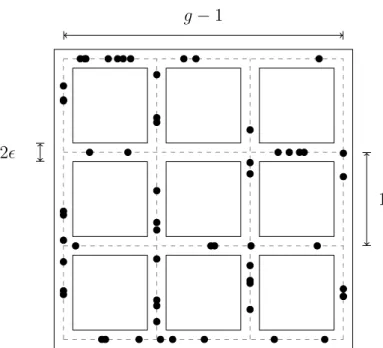
We already introduced the environment with two parameters, namely, the gran-ularityg and the segments’ width ǫ. Before proceeding to introduce the network that will operate on this environment, let us first to take a visual representation of the environment. Figure 2.1 presents a grid of granularityg = 4. Notice that segments are of unitary length whilst the respective common width is 2ǫ, for all of them.
We perceive, also in Figure 2.1, that all these segments have a central dashed line. In the model, nodes are deployed over these lines uniformly at random with intensity enough to generate an expected amount of nodes per segment equivalent to µ. In order to warrant the desired uniformity and density, we proceed to deploy the nodes as follows:
2.1. Geometric Layer 11
g−1
2ǫ
1
Figure 2.1. The geometrical layer: an urban obstructed environment with nodes deployed uniformly at random. The environment is defined by the granularity
g= 4 and the segments’ width parameter ǫ.
of nodes is determined by n = 2g(g−1)µ;
2. We create a vector, denoted byS, ofn elements coming from a uniform standard distribution. This vector represents an sample of the family{Si}1≤i≤nof indepen-dent and iindepen-dentically distributed (i.i.d.) random variables, such that Si ∼ U(0,1); 3. We proceed similar as the previous step, creating a vector, denoted by N, of n
elements coming from a random discrete uniform distribution defined on the set {1,2, . . . ,2g(g−1)};
4. We use any bijection fd(.) from {1,2, . . . , n} to the set of segments in the grid and, for all node i ∈ {1,2, . . . , n} we deploy i in the segment fd(N[i]), in the locally referenced position S[i] of that specific segment.
As we anticipated at the beginning of this chapter, a second aspect for modeling a wireless ad hoc network consists on defining the rules of communication, that is, the rules that determine the existence of links between nodes. In general, we say that two nodes uand v are able to communicate through a link if and only if (iff) we satisfy (i) a power restriction and (ii) there exist a path for the signal to arrive from one node the the other.
12 Chapter 2. Model
signal fades with the distance to the power of the path loss. Consequently, when a nodeutransmit a message to node v, we say thatv is able to receive it if the strength of the signal, perceived at the position of v, divided by the strength of interferences from other transmissions that occur simultaneously plus the ambient noise, exceeds some hardware dependent thresholdβ.
As Lotker and Peleg [2010] pointed out, a high amount of research exists on the SINR model and other variants of the so-called physical model, yet progress has been rather slow. This is a consequence of the non-triviality of this model for being incorporated in the analysis of communication protocols and network design. Added to these difficulties, we are in a more complex case with the presence of objects that reflect the signal in different manners.
Accordingly, we adopt a widely accepted abstraction for wireless communication, known as the Unit Disk Graph (UDG) model [Huson and Sen, 1995], and adapt it to our obstructed urban environment. The UDG model states that a message sent by node u is received by every other listening node v positioned within a disk, of radius
r, centered at the position of u. Additionally, since we are considering homogeneous networks, the radius r is restricted to be a common transmission range, depending of the power with which nodes in the network transmit.
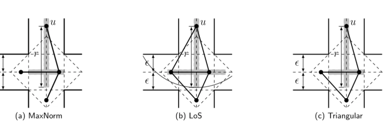
More specifically, we define three different geometric models to determine whether local communication links exist between two nodesuandv. Let us denote the positions ofuandv with (xu, yu) and (xv, yv), respectively. Note that the existence of such links depends on two criteria: distance and visibility. Also, the most challenging scenario in terms of visibility is when the two nodes are located in perpendicular segments sharing an intersection. This happens because if they are in the same segment, then only the distance criterion counts, and, if they are in parallel but non-successive segments, they are never visible to each other.
We synthesize the three models as follows:
MaxNorm model: uand v are able to communicate with each other if the following two conditions are satisfied: (i) the minimum norm min{kxu −xvk,kyu −yvk} does not exceed ǫ, and (ii) the maximum norm max{kxu −xvk,kyu −yvk} does not exceed the common transmission range r (see Figure 2.2a). Informally, this model states that to satisfy the visibility criterion between nodes in perpendicular segments, at least one node of{u, v} must be located inside the square of side 2ǫ
centered at the intersection of segments.
com-2.1. Geometric Layer 13
ǫ
ǫ
u
r
(a) MaxNorm
ǫ
ǫ
u
r
(b) LoS
ǫ
ǫ
u
r
(c) Triangular
Figure 2.2. Determining the communication links present at street intersections. The gray region represents the coverage of node u.
mon transmission range r, and (ii) there is a visibility line between u and v (see Figure 2.2b). Note that this model makes no simplifications when establishing visibility between two nodes in perpendicular segments, i.e., all possible place-ments of {u, v}in perpendicular (and adjacent) segments must be considered.
Triangular model: uand v are able to communicate with each other if the following two conditions are satisfied: (i)uandv are connected in the MaxNorm model, or (ii) both uand v are at most at a distance 2ǫ far from a shared intersection (see Figure 2.2c). This model greatly simplifies the definition of visibility between two nodes in perpendicular street segments. It extends the MaxNorm model by stating that if both u and v are located inside the rhombus of diagonal 4ǫ, they are visible to each other. Note that this model has a higher similarity with LoS than the MaxNorm model has, since a significantly larger area and, consequently, more links are considered.
For determining a link between two nodes located in the very same or in successive segments, there is no distinction between the variants of communication models. On the other hand, when two nodes are located at segments perpendicular to each other, then the three models above offer a different criterion to determine the existence of a link. Figure 2.2 shows an example where the communication graph, of a deployed network, changes under the different models. Observing this figure, we perceive that the LoS model tends to be the most permissive, that is, the one that “accepts” more link for a given deployment.
14 Chapter 2. Model
we can treat connectivity by cases dividing the segments in two sectors: [0, ǫ] and (ǫ,1]. Nevertheless, having the LoS model as a reference, the main weakness of the Max-Norm model takes place when are nearǫ but in the interval (ǫ,1], and the transmission range
ris bigger than the distance between them. In this case, nodes can see each other, and they are close to each other, but the Max-Norm does not consider that link.
In response to the main weakness of the Max-Norm model, the Triangular model came for considering those links. In order to maintain a simple model for analytical treatment, we assume r ≥ √8ǫ. Consequently, we can treat connectivity by cases as before, but in this model we should divide the segments in three sectors: [0, ǫ], (2ǫ, ǫ] and (2ǫ,1].
2.2
Percolation Layer
As previously mentioned, we abstract the obstructed network using adiscrete percola-tion theory [Grimmett, 1999]. This theory, originally introduced simply as percolation theory1, was proposed by Broadbent and Hammersley [1957] after the work they had
done for optimal design of filters in gas mask during the World War II. According to Franceschetti and Meester [2007], the gas mask of the time used granules of acti-vated charcoal, and Broadbent and Hammersley perceived that the optimal functioning of the gas mask occurred while using a high charcoal surface area and tortuous paths from one extreme to the other, allowing the air flow through the canister for sufficient time and contact to absorb the toxin.
Few years later, the work of Broadbent and Hammersley was generalized by Gilbert [1961] in the context of radio communication. He introduced a model of random planar networks in continuum space, considering a network of nodes randomly distributed in the plane and connecting, through a communication link, nodes for which mutual distance is no bigger than a certain threshold. He proved the existence of a critical transmission range that induces and infinite chain of connected nodes. Additionally, he proved that, below this critical transmission range, any connected component of the network is bounded, that is, it is finite.
As we presented above, the discrete percolation model was introduced to study the maximum impermeability (for minimizing the penetration of toxins inside of the mask) that allows the flow of air through a canister with granules of activated charcoal. On the other hand, the continuum percolation model was introduced to study the possibility 1This mathematical framework was baptized under the name of percolation theory, since
2.2. Percolation Layer 15
(a) An instance of the gridG8 for pb= 1.
This case contains all possible edges be-tween vertices.
(b) An instance of the gridG8forpb= 0.45.
Figure 2.3. Intances of the random gridG8, withV={1,2, . . . ,8}2, while using
two different values for the probability of edges in a bond percolation model.
of providing long-distance radio connections using a large number of low-power radio transmitters. The core motivation in both percolation models was the same: provide a critical value for a parameter, p=pc, beyond which connectivity is warranted w.h.p., and under which any setting p < pc generates, w.h.p., fragmentation in the system.
Technically, we abstract the obstructed network through a discrete mixed per-colation model, which is a combination between the bond and site percolation mod-els [Grimmett, 1999]. In the following, we start by defining the random grid for both versions (bond and site percolation). This is the regular grid structure over which percolation is defined.
Consider the graph Gg = (V,E). The bond percolation model is defined on Gg
as follows:
1. We define V = {1,2, . . . , g}2 as the vertices of the grid. The position of each
vertex (x, y)∈V is defined by means of its indices (line and column in the grid)
over the Euclidean plane;
2. For each pair of nodesuand v wherekxu−xvk+kyu−yvk ≤1, we add the edge (u, v) to the set ❊with probability pb, independently of the rest of edges.
Figure 2.3 presents instances of the random lattice square G8 using two different
values of pb. Notice that, in Figure 2.3a, each one of the possible edges of the lattice occurs with maximum probability pb = 1. In Figure 2.3b we show an instance of G8
16 Chapter 2. Model
(a) An instance of a random grid for the site per-colation model, constructed withps= 0.45.
(b) Every instance of a random grid for the site percolation model can be seen as an instance of a random grid for the bond percolation model.
Figure 2.4. An instance of a random grid for the site percolation model with
g= 8, and the relationship with an instance of a bond percolation model.
a “closed edge”. The general rule of association with the “open” and “closed” words is (i) “open” means“connected” and (ii) “closed” means “disconnected”.
Another kind of random grid can be obtained by considering each box of the lattice square to be occupied (or equivalently, open) with probabilityps, independently of the rest of boxes, and available (or equivalently, closed) with probability 1−ps. Connections in this model have place between these open boxes, also known as “sites”, and we say that two sites are connected if they share a side, that is, if they are neighbours.
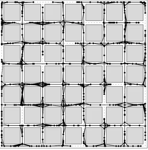
Figure 2.4a shows an instance of a random grid of size 8×8 corresponding to a site percolation process withps = 0.45. Each gray square box in this figure corresponds to an open site, and white spaces represent closed sites. We can think of sites as being vertices and then, adding edges between pairs of nodes that share a side, we obtain an instance of a bond percolation model, as Figure 2.4b shows. In this figure, open sites are plotted with filled bullets and closed sites with empty bullets. We ad an edge between two vertices whenever the vertices are open and have a common side.
Notice that instances of bond percolation processes cannot, in general, be viewed as coming from a site percolation process. For example, an instance of a bond per-colation process on G2 resulting with three edges does not represent any instance of
2.2. Percolation Layer 17
Figure 2.5. An extension of the bond percolation instance of Figure 2.3b with site probability ps=pb= 0.45.
percolation.
The discrete mixed percolation model is a bond percolation model, with param-eter pb, where the set of vertices can be open with probabilityps, independently of the rest of vertices, or closed with probability 1−ps. Taking the bond percolation instance of Figure 2.3b, we obtain the mixed percolation instance of Figure 2.5 by setting the open site probability ps= 0.45.
We already defined three percolation models and, in order to establish a rela-tionship with the geometrical layer of Section 2.1, we need then to define the concept of connectivity. Under the bond percolation model the random grid is connected, for a given instance, if there exists a sequence of vertices connected successively through open edges, staring at i and finishing at j, for any pair of vertices i and j. On the other hand, under the site percolation model the random grid is connected, for a given instance, if all open sites are connected through successive open sites sharing a side. Finally, the random grid is connected under the mixed percolation model, for a given instance, if for any pair of open vertices or (equivalently) sites i and j, there exists a sequence of open vertices and open edges starting at iand finishing at j.
18 Chapter 2. Model
segments is equal in all the segments and independent of the connectivity of other segments. The same applies to the probability of connectivity at intersections.
The aforementioned similarities allow us to construct the following abstraction: 1. We compute the probability of connectivity at intersections, denoted by Pr(Icon),
and the probability of connectivity at segments, denoted by Pr(Scon);
2. Under the mixed percolation model, we define the parameter ps to be Pr(Icon),
and we set the parameter pb to Pr(Scon);
3. We determine the critical values of pb and ps that warrant connectivity in the random grid w.h.p.;
4. For Pr(Icon) and Pr(Scon), we characterize the transmission range r, density µ
and segments’ width parameterǫ that generate the critical values for percolation w.h.p. in the random grid.
After step 4, the characterizations of r, µ and ǫ that generate a certain property, let us say connectivity for instance, match with the characterizations for the equivalent property under the communication network. The more relevant case, and the main for this thesis, corresponds to the characterization of critical value for connectivity, known as the critical value for percolation under the grid, and introduced as the CTR for connectivity in the communication network.
Next chapter is dedicated to the derivation of expressions for Pr(Scon) and for
Pr(Icon) under the three communication models presented in the geometrical layer.
Chapter 3
Local Connectivity Probabilities
Connectivity is one of the most important properties in ad hoc wireless networks since it allows basic communication between the nodes that constitute the network. There are two different instances of wireless communication: direct and multi-hop. Direct communication between two nodes occurs when they are able to exchange information without any intermediary. On the other hand, multi-hop communication has place when it is possible to find a path from one node to the other, passing through different intermediate nodes are able to exchange information, in pairs, using direct communi-cation.
The possibility of wireless direct communication relies on complex physical phe-nomena, and the literature tradition is to abstract this complexity using diverse connec-tivity models that allow us to work analytically on different problems. As anticipated in Chapter 2, we consider a distance-based model for communication in one-dimensional problems (for connectivity at segments), and three different geometric models for two-dimensional cases (for connectivity at intersections).
In the next two sections, we derive analytical expressions for the probability of connectivity at intersections and segments, respectively. These two events are the building blocks used to solve connectivity in the overall network.
3.1
Probability of Connectivity at Intersections
As we saw in Section 2.1, we treat the problem of connectivity at intersections under three different models. Probabilities related to connectivity at intersections under the Max-Norm model are presented in Section 3.1.1. Analytical formulation for the LoS model is included in Section 3.1.2. Then, we present a derivation of the probability of connectivity at intersections under the Triangular model in Section 3.1.3.
20 Chapter 3. Local Connectivity Probabilities
1 1
1
1
r
r r
r
2ǫ
2ǫ
2ǫ
2ǫ
X(1)X(2) · · · X(µ) Y(1)
Y(2)
.. .
Y(µ)
W(1)
W(2)
· · · W(µ)
Z(1)
Z(2)
.. .
Z(µ)
Figure 3.1. Reference scenario for connectivity at intersections
Before entering in details with any of the three models, let us first to introduce a reference scenario that defines with more precision the elements to be considered while computing connectivity at intersections.
We consider the reference scenario illustrated in Figure 3.1, where µ nodes are deployed uniformly at random, in each one of the four adjacent segments of an inter-section, over imaginary lines centered in each segment. All the 4µ nodes share the same transmission range r, and segments’ width is 2ǫ, where ǫ is the parameter that controls the visibility between nodes deployed in perpendicular segments.
In the aforementioned reference scenario, the communication net-work can be represented as a graph G = (V, E), where V = {X1, . . . , Xµ, Y1, . . . , Yµ, W1, . . . , Wµ, Z1, . . . , Zµ}, and the set of edges E is com-posed by pairs of nodes that are able to communicate with each other in the network, according to each one of the three connectivity models.
Let us define now a new graph I = (V,E) with V = {X, Y, W, Z}, where X =
{X1, . . . , Xµ},Y ={Y1, . . . , Yµ},W ={W1, . . . , Wµ}andZ ={Z1, . . . , Zµ}, and where
hA, Bi ∈E iff there exist i∈ A and j ∈B such that hi, ji ∈ E, that is, iff hi, ji is an
edge inG. We call this new graph theIntersection Graph.
Problem 1 (Connectivity at Intersections). The connectivity at intersections prob-lem consists in determining the probability of connectivity of the intersection graph I, namely Pr(Icon).
Nodes under the same gray area in Figure 3.1 represent the four set of nodes X,
3.1. Probability of Connectivity at Intersections 21
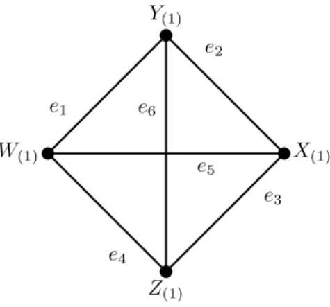
X(1)
Y(1)
W(1)
Z(1)
e1
e2
e3
e4
e5
e6
Figure 3.2. Intersection Graph
when the biggest connected component in G is smaller than four, i.e., we just need to connect the four nodes in I. Additionally, we observe that there is a link hA, Bi in the intersection graph iff there is a link between the closest nodes to the intersection in the original graph G. These nodes are know to be the first order statistics, and are denoted, in this case by A(1) and B(1), respectively.
Figure 3.2 shows the intersection graph. Here, we use the “(1)” subscript to
emphasize the fact that edges between nodes in the intersection graph are present iff there exist a link between the corresponding first order statistics in the network. We number random edges frome1 toe6 from now on according to Figure 3.2 to simplify the
treatment in the moment of computing the probability of connectivity at intersections. In the network, we distinguish between links connecting nodes positioned in paral-lel and perpendicular segments. We denote bypk the probability of existence of an link between two nodes located in parallel segments sharing an intersection. On the other hand, p⊥ denotes the probability of existence of a link between two nodes positioned in perpendicular segments sharing an intersection. We extend these two definitions to the probability of existence of at least one link between groups of µ nodes, and we denote this extension by pk(µ) and p⊥(µ).
3.1.1
Max-Norm Model
The Max-Norm is the simplest of the three proposed models, and we proceed to com-pute some connectivity probabilities having as a final goal to comcom-pute the probability of connectivity at intersections under the Max-Norm model, denoted by Pr(IMN
con).
We can think the event IMN
con as being the set instances of the intersection graph
that connect the four nodesX(1),Y(1),W(1) andZ(1) (see Figure 3.2). Individually, the
22 Chapter 3. Local Connectivity Probabilities
adjacent edges are spatially correlated,the probability of collective occurrence is not simple to compute (correlation results from the fact that adjacentexternal edges share a node). Differently, edges e5 and e6 are mutually independent, and the individual
probability of occurrence is denoted by pk(µ). Although edges e5 and e6 are mutually
independent, they are not collectively independent with any of the other edges, from
e1 toe4.
In the following we present an accurate approximation of the probability pk(µ) fore5. Since the probability ofe6 is the same as the one corresponding toe5, Lemma 1
we presents the general result. Here, and in the rest of the work, position of nodes are relative to the origin of intersection, this means the the support for random variables is on the interval [0,1].
Lemma 1. Let{Xi}1≤i≤µ and {Wj}1≤j≤µ be two families of independent random
vari-ables, such that Xi ∼ U(0,1)§ and Wj ∼ U(0,1), denoting the positions of µ nodes
in each one of two parallel segments sharing an intersection. Let also r denote the common transmission range of all nodes, where 0 ≤ r ≤ 1. The probability pk(µ) of existence of at least one link between two nodes in parallel adjacent segments is
pk(µ)≈ r 6
µ−µ(1−r)µ−4µ1− r 2
µ−1
1− r 2
µ
−1
.
Proof. Sorting the realizations ofX1, X2, . . . , Xµand W1, W2, . . . , Wµ in increasing or-der, we obtain the order statistics¶ X(1), X(2), . . . , X(µ) and W(1), W(2), . . . , W(µ),
re-spectively. W.l.o.g., we consider that positions of nodes reflect the Euclidean distances from each node to the intersection point between segments.
At least one crossing link between two nodes positioned in different parallel seg-ments exists if and only ifX(1)+W(1) ≤r. Then, we can compute pk(µ) by
pk(µ) =
Z Z
D
fX(1)W(1)(x, w) dwdx, (3.1)
where D = {(x, w) | 0 ≤ x ≤ r∧0 ≤ w ≤ r−x} and fX(1)W(1)(x, w) is the joint
distribution function of X(1) and W(1). Figure 3.3 draws integration region according
to the restrictionX(1)+W(1) ≤r.
It is well known that thek-th order statistic of a family ofµindependent standard uniform random variables is a Beta random variable U(k) ∼ B(k, µ+ 1−k).
Conse-quently, we have that fX(1)(x) =µ(1−x)
µ−1 and f
W(1)(w) =µ(1−w)
µ−1. Since both
§I.e., distributed uniformly and at random in the interval [0
,1].
¶The
3.1. Probability of Connectivity at Intersections 23
X(1)
W(1) r−x
r r
Figure 3.3. Integration region Dfor computing pk(µ)
families {Xi}1≤i≤µand {Wj}1≤j≤µare independent, we have that the joint distribution function of X(1) and W(1) isfX(1)W(1)(x, w) =µ
2(1−x)µ−1(1−y)µ−1. Then, replacing
fX(1)W(1)(x, w) in Equation (3.1), we have
pk(µ) =
Z r
0
Z r−x
0
µ2(1−x)µ−1(1−w)µ−1dwdx
=
Z r
0
µ −(1−x)µ−1
((−r+x+ 1)µ−1) dx. (3.2)
At this point, we are not able to solve the integration of Equation (3.2), so we apply an approximation method known as the Simpson’s rule. Applying this Simpson’s rule with two intervals, we have
pk(µ)≈ r 6
µ−µ(1−r)µ−4µ1− r 2
µ−1
1− r 2
µ
−1
.
Notice that in any moment during demonstration of Lemma 1 we assume a prop-erty that holds specifically under the Max-Norm model, which implies thatpk(µ) is the same for the three models addressed in this manuscript.
Figure 3.4 presents the probability of crossing links between parallel segments sharing an intersection in three scenarios, determined by the parameter µ. Here we perceive that the approximation we obtained, using Simpson’s rule with two intervals in (3.2), is an accurate expression for pk(µ).
24 Chapter 3. Local Connectivity Probabilities
r pk
(
µ
)
0.0 0.2 0.4 0.6 0.8 1.0
0.0 0.4 0.8
µ= 1
0.0 0.4 0.8
µ= 3
0.0 0.4 0.8
µ= 5
Figure 3.4. Empirical and analytical results for pk(µ) under the Max-Norm model
of at least one link between two groups of µ nodes positioned in its two respective segments sharing an intersection. In the derivation, we assume specific properties related to the Max-Norm model, and we denote the exact probability of existing at least one crossing link between perpendicular segments by pMN
⊥ (µ), emphasizing this fact.
Lemma 2. Let {Xi}1≤i≤µ, such that Xi ∼ U(0,1), and {Yj}1≤j≤µ, such that Yj ∼ U(0,1), be two families of independent random variables denoting the position of µ
nodes in each one of two perpendicular segments sharing an intersection. Let also 2ǫ
be the segments’ width, and r denote the common transmission range of all nodes, where ǫ ≤ r ≤ 1. The probability pMN
⊥ (µ) of existence of at least one link between two
nodes in different perpendicular segments, under the Max-Norm model, is
pMN
⊥ (µ) = 2 (1−(1−r)µ) (1−(1−ǫ)µ)−(1−(1−ǫ)µ)
2
.
Proof. Let X(1), X(2), . . . , X(µ) and Y(1), Y(2), . . . , Y(µ) be the order statistics of
3.1. Probability of Connectivity at Intersections 25
X(1)
Y(1)
y=x
ǫ ǫ
r r
(a) General integration regionD
X(1) Y(1) ǫ ǫ r r
(b) Integration regionR1
X(1) Y(1) ǫ ǫ r r
(c) Integration regionR2
Figure 3.5. Integration region D, and alternative partition for computing
pMN
⊥ (µ)
Considering ǫ≤r, we can compute pMN
⊥ (µ) by
pMN
⊥ (µ) =
Z Z
D
fX(1)Y(1)(x, y) dydx, (3.3)
where D is the region showed in Figure 3.5a andfX(1)Y(1)(x, y) is the joint distribution
function of X(1) and Y(1).
It is important to highlight that the join distribution function of two equally distributed random variables is symmetric respect to the y =x plane in the Euclidean space. Since region D is symmetric respect to line y=x and, additionally, fX(1)Y(1) is
symmetric respect to plane y = x, we can decompose integral of equation (3.3) into regions as follows:
pMN
⊥ (µ) = 2
Z Z
R1
fX(1)Y(1)(x, y) dydx−
Z Z
R2
fX(1)Y(1)(x, y) dydx, (3.4)
where R1 ={(x, y)|0≤x≤r∧0≤y≤ǫ} and R2 ={(x, y)|0≤x≤ǫ∧0≤y≤ǫ}
(see Figure 3.5).
Since X(1), Y(1) ∼ B(1, µ) are independent, the joint distribution function is
fX(1)Y(1) =µ
2(1−x)µ−1(1−y)µ−1. Then, from (3.4), we have
pMN
⊥ (µ) = 2
Z r
0
Z ǫ
0
µ2(1−x)µ−1(1−y)µ−1dydx−
Z ǫ
0
Z ǫ
0
µ2(1−x)µ−1(1−y)µ−1dydx
26 Chapter 3. Local Connectivity Probabilities
r
p
M
N
⊥
(
µ
)
0.6 0.7 0.8 0.9 1.0
0.4 0.6 0.8
µ= 5
ǫ= 0.25
µ= 7
ǫ = 0.25
0.4 0.6 0.8
µ= 9
ǫ= 0.25
µ= 5
ǫ= 0.35
0.4 0.6 0.8
µ= 7
ǫ = 0.35
0.6 0.7 0.8 0.9 1.0
µ= 9
ǫ= 0.35
Figure 3.6. Probability of connectivity between nodes located at perpendicular segments sharing an intersection
For the case of crossing links between perpendicular segments, we have selected six scenarios, varying the segment width parameter, ǫ, and the expected number of nodes per segment, µ. Figure 3.6 presents these results considering the assumption
r≥ǫfrom Lemma 2. It can be seen that the expression obtained forpMN
⊥ (µ) is correct. At this stage, we have already computed the probability of existence of at least one crossing link between parallel segments,pk(µ), and perpendicular segments,pMN
⊥ (µ). The next step is to compute the probability of connectivity at intersections, namely Pr(IMN
con). Somehow, this probability can be described by a (non-trivial) function of
pk(µ) and pMN
⊥ (µ), which takes into account the geometric correlation between the ex-istence of simultaneous links between both, parallel and perpendicular segments. Nev-ertheless, we perceive in Almiron et al. [2012] that the influence ofpk(µ) on Pr(IMN
con) is
seg-3.1. Probability of Connectivity at Intersections 27
ments sharing an intersection. An exception to this behavior is when µ or ǫ are very small values, which are scenarios not so relevant in practice. An example of this occurs in the CTR problem, where we want to use the minimum radio for communication as possible while maintaining connectivity in the overall network. Clearly, in this prob-lem, small densities and low visibility at intersections implies too large communication radios, which is not of practical interest for nowadays technological environments. For the reason above and for the sake of simplification, in Theorem 1, we compute a lower bound on Pr(IMN
con) using onlypMN⊥ (µ). After this, in Theorem 2, we present an accurate
expression for Pr(IMN
con) but, at this time, considering links between both, parallel and
perpendicular segments.
Theorem 1. Let{Xi}1≤i≤µ,{Yj}1≤j≤µ, {Wk}1≤k≤µ and{Zm}1≤m≤µ be four families of
independent random variables, such that Xi ∼ U(0,1), Yj ∼ U(0,1), Wk ∼ U(0,1) and Zm ∼ U(0,1), denoting the positions of µ nodes in four adjacent segments sharing an
intersection. Let also 2ǫ be the segments’ width andr denote the common transmission range of all nodes, with ǫ≤ r ≤1. A lower bound of the probability of connectivity at intersections, denoted by Pr(IMN
con), is given by
Pr(IMN
con)≥2ξ
2
− ξ
4
p2 +p
2, (3.5)
where ξ= ((1−ǫ)µ−1)((1−r)µ−(1−ǫ)µ) and p=pMN
⊥ (µ).
Proof. W.l.o.g., we consider that positions of nodes reflect the Euclidean distances from each node to the intersection point between segments. Consider the order statis-tics X(1), Y(1), W(1) and Z(1), from the families {Xi}1≤i≤µ, {Yj}1≤j≤µ, {Wk}1≤k≤µ and {Zm}1≤m≤µ, respectively. There exists a path between at least one node in a segment connecting at least one node in each one of the three other segments if and only if there exists a path between X(1), Y(1),W(1) and Z(1).
Considering only links between perpendicular segments, we can obtain a lower bound as follows. Lete1 be the event that indicates the presence of a link between the
realizations of Y(1) and W(1) (see Figure 3.2, in page 21). Additionally, lete2,e3 ande4
represent the existence of a link between X(1) and Y(1), X(1) and Z(1) and finally W(1)
and Z(1), respectively. Since X(1),Y(1), W(1) and Z(1) are independent, we have e1⊥⊥e3
and e2⊥⊥e4, where ⊥⊥ indicates the stochastic independence between events. Consider
now the experiment of observing the presence ofe1 ande3 simultaneously. The sample
space of this experiment can be partitioned by Ω = {e1∩e3, e1 ∩e3, e1 ∩e3, e1 ∩e3}.
28 Chapter 3. Local Connectivity Probabilities
bound by
Pr(IMN
con)≥Pr(IconMN |e1∩e3)p2+2 Pr(IconMN|e1∩e3)p(1−p)+Pr(IconMN|e1∩e3)(1−p)2, (3.6)
wherep= Pr(e1) = Pr(e3) =pMN⊥ (µ).
Notice that Equation 3.6 does effectively represent a lower bound, since links between nodes positioned in parallel segments are not considered in the expression. This restriction has an immediate consequence: the third term of Equation 3.6 does not contribute to connectivity, because there is no way to have connectivity at intersections without e1 nor e3. Then, we only need to find expressions for Pr(IconMN | e1∩e3) and
Pr(IMN
con |e1∩e3). Lets consider Pr(IconMN |e1∩e3) first.
We can solve Pr(IMN
con |e1∩e3) considering probabilities of three cases under which
we achieve connectivity at intersections: (i) both,e2 ande4 occur, (ii)e2 occurs ande4
does not and (iii)e2 does not occur ande4does. Since cases (ii) and (iii) are symmetric,
we have
Pr(IMN
con |e1 ∩e3) = Pr(e2 |e1∩e3)2+ 2 Pr(e2 |e1∩e3) (1−Pr(e2 |e1∩e3)). (3.7)
Additionally, we have
Pr(e2 |e1∩e3) = 1−Pr(e2 |e1∩e3)
= 1−Pr(ǫ≤X(1) ≤r∩ǫ≤Y(1) ≤r∩e1∩e3) Pr(e1∩e3)
. (3.8)
Sincee1⊥⊥e3, we can rewrite (3.8) and solve
Pr(e2 |e1∩e3) = 1−
Rr
ǫ
Rǫ
0fX(1)Z(1)(x, z) dzdx
2
p2
= 1− ((1−ǫ)
µ−1)2((1−r)µ−(1−ǫ)µ)2
p2 . (3.9)
In order to solve the lower bound for Pr(IMN
con) proposed in (3.6), we still need to
compute Pr(IMN
con | e1 ∩e3). Notice that even in the case where we do not have e3, we
still need X(1) ≤ r and Z(1) ≤ r, otherwise we are not able to achieve connectivity at
intersection. Being aware of this, we know then that ǫ < X(1) ≤ r and ǫ < Z(1) ≤ r.
This is because we do not want to give a chance to have e3 while we are actually
conditioning one1∩e3. We all these considerations, we can then compute
Pr(IMN
3.1. Probability of Connectivity at Intersections 29
whereA ={0≤Y(1) ≤ǫ∩0≤W(1) ≤ǫ∩ǫ ≤X(1) ≤r∩ǫ≤Z(1) ≤r}. SinceY(1)⊥⊥e3,
W(1)⊥⊥e3, X(1)⊥⊥e1 and Z(1)⊥⊥e1, from (3.10) we have
Pr(IMN
con |e1∩e3) =
Z ǫ
0
Z ǫ
0
fY(1)W(1)(y, w) dwdy
Z r
ǫ
Z r
ǫ
fX(1)Z(1)(x, z) dzdx
1
p(1−p). (3.11) Solving the definite integrals in (3.11), we obtain
Pr(IMN
con |e1∩e3) =
((1−ǫ)µ−1)2((1−r)µ−(1−ǫ)µ)2
p(1−p) . (3.12)
Finally, combining (3.7), (3.9) and (3.12) within Expression (3.6), and considering
ξ = ((1−ǫ)µ−1)((1−r)µ−(1−ǫ)µ) we finally have
Pr(IMN
con)≥2ξ2−
ξ4
p2 +p 2.
Although Theorem 1 considers only links between nodes located in perpendicular segments sharing an intersection, the obtained lower bound was not an expression as simple as we would like. This last fact, encouraged us to find a solution considering all links, that is, not just those between nodes in perpendicular segments, but those between nodes located in parallel segments as well.
Theorem 2 presents a tight lower bound for Pr(IMN
con) considering all links at a
given intersection.
Theorem 2. Let{Xi}1≤i≤µ,{Yj}1≤j≤µ, {Wk}1≤k≤µ and{Zm}1≤m≤µ be four families of
independent random variables, such that Xi ∼ U(0,1), Yj ∼ U(0,1), Wk ∼ U(0,1) and Zm ∼ U(0,1), denoting the positions of µ nodes in four adjacent segments sharing an
intersection. Let also 2ǫ be the segments’ width andr denote the common transmission range of all nodes, with 2ǫ≤r ≤1. A lower bound of the probability of connectivity at intersections, denoted by Pr(IMN
con), is given by
Pr(IMN
con)≥p
2+ 2Dǫ
0(µ)Drǫ(µ)Drǫ−ǫ(µ) [Dr0(µ) +Drǫ(µ)], (3.13)
where Dji(k) = (1−i)k−(1−j)k and p=pMN
⊥ (µ).
30 Chapter 3. Local Connectivity Probabilities
W(1) and Z(1), from the families {Xi}1≤i≤µ, {Yj}1≤j≤µ, {Wk}1≤k≤µ and {Zm}1≤m≤µ, respectively. The intersection graph I is connecterd iff there exists a path between
X(1), Y(1), W(1) and Z(1).
Consider events e1, e2, e3, e4, e5 and e6, from Figure 3.2 (page 21), as being the
events that indicates the presence of a link between the realizations of Y(1) and W(1),
X(1) and Y(1), X(1) and Z(1), W(1) and Z(1), X(1) and W(1), and finally Y(1) and Z(1),
respectively. Let us highlight thate1⊥⊥e3 and e2⊥⊥e4, and that pairs of edges sharing
a node are clearly not independent because of geometrical correlation. In particular, sincee1⊥⊥e3, we are able to construct the partitionPe={e1∩e3, e1∩e3, e1∩e3, e1∩e3}
on the sample space Ω (the set of all possible combinations of nodes positions). Consequently, applying the law of total probability and considering the symmetry betweene1 ∩e3 and e1∩e3 , we can compute
Pr(IMN
con) = Pr(I
MN
con |e1∩e3) Pr(e1 ∩e3) + 2 Pr(IconMN|e1∩e3) Pr(e1∩e3)
+ Pr(IMN
con |e1∩e3) Pr(e1∩e3) (3.14)
The three summands in (3.14) contain the eventIMN
con conditioned one1∩e3,e1∩e3
or e1 ∩e3. To solve these probabilities, we use a second partition with bounds on ǫ
and r,
Pǫ,r = {0 ≤ W(1) ≤ ǫ, ǫ < W(1) ≤ r} × {0 ≤ Z(1) ≤ ǫ, ǫ < Z(1) ≤ r}, (3.15)
and apply the law of total probability one1∩e3,e1 ∩e3 and e1∩e3, respectively. We
identify two intervals, in (3.15), where W(1) and Z(1) belong to [0, ǫ] and (ǫ, r]. We
call these two intervals asS1 andS2, respectively, and define Ci,j as being the element of partition Pǫ,r where W(1) ∈ Si and Z(1) ∈ Sj. With this partition, we proceed to compute each conditional term of (3.14).
Let us consider firstly the partition Pǫ,r on e1 ∩e3 for solving Pr(IconMN | e1∩e3).
Figure 3.7a shows a schematic view of partition Pǫ,r on e1∩e3, where the black balls
represent instances of W(1) and gray balls represent instances of Z(1). Each pair of
balls of different color represent a classCi,j of Pǫ,r. Edges, in this figure, represent the conditioning on e1 ∩e3, and the position of stars represent the worst case (farthest
region from the origin) for this conditioning. Numbering in both, balls and stars, is used for identifying the intervals of instances of W(1) and Z(1), and more important,