Lat. Am. j. solids struct. vol.11 número7

(1)

Abs tract

In this paper a new hybrid glowworm swarm algorithm (SAGSO) for solving structural optimization problems is presented. The structure proposed to be optimized here is a simply-supported concrete I-beam defined by 20 variables. Eight different concrete mixtures are studied, varying the compressive strength grade and compacting system. The solutions are evaluated following the Spanish Code for structural concrete. The algorithm is applied to two objective functions, namely the embedded CO2 emissions and the economic cost of the structure. The ability of glowworm swarm optimization (GSO) to search in the entire solution space is combined with the local search by Simulated Annealing (SA) to obtain better results than using the GSO and SA independently. Finally, the hybrid algorithm can solve structural optimization problems applied to discrete variables. The study showed that large sections with a highly exposed surface area and the use of conventional vibrated concrete (CVC) with the lower strength grade minimize the CO2 emissions.

Key words

Hybrid glowworm swarm algorithm, discrete variables, concrete I-beam, CO2 emissions, self-compacting concrete.

Optimization of concrete I-beams using a new hybrid

glowworm swarm algorithm

1 INTRODUCTION

The traditional goals of engineers are the design of safe and economic structures. However, there is a growing concern for sustainability about the need to protect the environment. Now, more than ever, engineers should choose environmentally-friendly materials and cross-section dimension to minimize the impact of their projects as well as the consumption of natural resources. In this con-text, the so-called metaheuristics methods have shown to be highly suited to design structures (Hare et al., 2013). While the design of economic structures has always been conditioned by the

Ta ti an a G arcía -Se g ura a V í cto r Y e pe s b, * Jos é V . Martí c Ju li án A l cal á d

a_{Graduate Research Assistant, ICITECH,}

Dept. of Construction Engineering, Universi-tat Politècnica de València, 46022 Valencia,

Spain.

b_{Associate Professor, ICITECH, Dept. of}

Construction Engineering Universitat Politèc-nica de València, 46022 Valencia, Spain.

Corresponding author. Phone +34963879563; Fax +34963877569.

c_{Associate Professor, ICITECH, Dept. of}

d_{Assistant Professor, ICITECH, Dept. of}

(2)

Latin American Journal of Solids and Structures 11 (2014) 1190-1205 experience of structural engineers, metaheuristic methods have recently provided efficient structures with a reasonable computing time.

Optimization of reinforced concrete (RC) structures has been investigated by many researchers in the past. A thorough review of nonheuristic structural concrete optimization studies can be found in Sarma and Adeli (1998). Many later studies have been undertaken to implement evolutionary algorithms to solve structural concrete optimization problems (Kicinger et al., 2005), while the pre-sent authors’ research group reported on non-evolutionary algorithms to optimize real-life RC struc-tures (Payá-Zaforteza et al., 2010; Yepes et al., 2012; Carbonell et al., 2012; Martí et al., 2013; Mar-tínez-Martín et al., 2013; Torres-Machí et al., 2013).

Swarm intelligence is a type of biologically-artificial intelligence based on neighbour interactions. It imitates the collective behaviour of some agents which follow a global pattern. They interact with one another and learn from it. In fact, these algorithms differ in philosophy from genetic algorithms because they use cooperation rather than competition (Dutta et al., 2011). Particle swarm optimiza-tion (PSO) simulates a simplified social system (Kennedy and Eberhart, 1995). Ant colony optimi-zation (ACO) was proposed by Colorni et al. (1991) simulating the behaviour of ants leaving pher-omone to guide others. Artificial bee colony (Basturk and Karaboga, 2006; Karaboga and Basturk, 2008) mimics the food forage behaviour of honeybees. The glowworm swarm optimization (GSO) algorithm was proposed by Krishnanand and Ghose (2009) to obtain multiple optima of multimodal functions. This algorithm imitates a glowworm carrying luciferin and moving towards a mate whose luciferin level is higher than its own (Liao et al., 2011; Gong et al., 2011; Luo and Zhang, 2011; Khan and Sahai, 2012). However, Qu et al. (2011) pointed out its low convergence rate; what is more, this algorithm can be effective for searching a local optimum, but some shortcomings exist for searching the global optimum solution (Zhang et al., 2010).

The main purpose of this paper is to demonstrate how the standard GSO can be improved by incorporating a hybridization strategy. A hybrid GSO algorithm (SAGSO) is proposed, combining the broad search ability of GSO and SA effectiveness to find a global optimum to speed up the local search. Hybrid GSO has already been proposed combining a simplex search method (Qu et al., 2011), chaos optimization mechanism (Zhang et al., 2010), Hooke-Jeeves pattern search (Yang et al., 2010) and differential evolution (Luo and Zhang, 2011). In fact, the results showed that the hybrid algorithm had faster convergence, higher accuracy and was more effective for solving con-strained engineering optimization problems (Luo and Zhang, 2011). Hybrid PSO optimization has also been widely applied (Shieh et al., 2011; Valdez et al., 2011; Fan and Zahara, 2007; Ahandania et al., 2012; Li et al., 2009; Wang et al., 2013) demonstrating faster convergence rates. Likewise, ACO was improved by incorporating a hybridization strategy (Chen et al., 2012; Koide et al., 2013).

This paper describes a new hybrid algorithm applied to two objective functions, namely the em-bedded CO2 emissions and the economic cost. For the design of a simply supported concrete

(3)

Latin American Journal of Solids and Structures 11 (2014) 1190-1205

2 THE OPTIMUM DESIGN PROBLEM

The structural design problem established for this study aims to minimize the objective function F

of equation (1), subject to the constraints represented by equation (2).

F

(

x

1

,

x

2

,...,

x

n

)

(1)

g

_j

(x

₁

,

x

₂

,...x

_n

)

_≤

0

₍₂₎

x

_i

_∈

d

_i₁

,d

_i₂

,...,d

_iq

i

(

)

(3)

Note that x1, x2,..., xn are the variables to be optimized (design variables). Each design variable

may assume the discrete values listed in equation (3). The objective function F defined in equation (1) is either the cost or the CO2 emission. The constraints gj in equation (2) are all the service limit

states (SLSs) and ultimate limit states (ULSs) with which the structure must comply, as well as the geometrical and constructability constraints of the problem. The following sections describe the problem in detail.

2.1 Design variables and parameters

The case considered here is a simply supported concrete I-beam (see Figure 1). The problem is for-mulated with 20 variables. Seven variables define the geometry: the depth (h), the width of superior flange (bfs), the width of inferior flange (bfi), the thickness of the superior flange (tfs), the thickness

of the inferior flange (tfi), the web thickness (tw) and the concrete cover (r). Another variable

estab-lishes the concrete mix: four mixes of SCC and four mixes of CVC represent four strength classes. The mixtures are described by Sideris and Anagnostopoulos (2013). All mixtures use crushed lime-stone.

Finally, passive reinforcement is defined by the number and diameter of the bars. The longitudi-nal reinforcement is arranged in longitudilongitudi-nal upper reinforcement (n1, Ø1), covering the whole beam

length. Lower reinforcement is divided in two systems, one covering the whole beam length (n2, Ø2)

and another covering the central part of the beam (n3, Ø3). Transversal and longitudinal shear

rein-forcement changes between two zones, support zone as length of L/5 near the supports and central zone. Shear reinforcement is defined by the number of bars per meter and their diameter in the support zone (n4, Ø4) and in the central zone (n5, Ø5). The number of bars per meter of transversal

and longitudinal shear reinforcement is equal, while the diameter can change. Therefore, four varia-bles define the longitudinal shear reinforcement: the support zone (n4, Ø6) and the central zone (n5,

(4)

Latin American Journal of Solids and Structures 11 (2014) 1190-1205 Figure 1 Design variables of the simply supported concrete I-beam.

The parameters of the I-beam are all fixed quantities that do not change during the optimiza-tion, including the beam span (15 m), the permanent distributed load (20 kN/m), and the variable distributed load (10 kN/m).

2.2 Structural constraints

Considering all the data necessary to define a given structure, the structural evaluation module calculates the stress envelopes and checks all the limit states and the geometric constraints repre-sented by equation (2). Serviceability and ultimate limit states (SLS and ULS) must be guaranteed following the Spanish Standard EHE-08 (Fomento, 2008). As for the instantaneous and time-dependent deflection of the central section, a limitation of 1/250 of the beam span for quasi-permanent loading conditions is imposed. Besides, if the section does not comply with the geomet-rical and constructability constraints, it is rejected.

One hundred years are required for the service life. The study was developed by evaluating du-rability according to the EHE code (Fomento, 2008). The code presents dudu-rability of a concrete structure as its capacity to withstand, for the duration of its designed service life, the physical and chemical conditions to which it is exposed. Carbonation is the main factor leading to RC decay. Service life of RC structures is assessed as the sum of two phases, according to equation (4). This mode is based on the Tuutti (1982) model. The first phase is initiation of corrosion, in which car-bonation penetration in the concrete cover means the loss of reinforcement passivity. The second phase involves the propagation of corrosion that begins when the steel is depassivated and ends when a limiting state is reached beyond which the consequences of corrosion can no longer be toler-ated.

t

₌

d

k

⎛

⎝⎜

⎞

⎠⎟

2

+

80 ⋅

d

ϕ ⋅

v

_c (4)

where, t are the years of service life; d is concrete cover (mm); k is the carbonation rate coefficient;

ϕ

is the bar diameter (mm), and vc is the corrosion rate (μm/year). The carbonation rate

(5)

values of the compressive strength and carbonation rate coefficient are presented in Table 1. In a general exposure, like IIb, the corrosion rate is about 2 μm/year (Fomento, 2008).

Table 1 Mix design properties and cement content.

Description Compressive strength (MPa) k (mm/year0.5) Cement (kg/m3)

Concrete SCC1 35.80 7.42 302

Concrete SCC2 45.30 5.14 336

Concrete SCC3 54.20 3.40 374

Concrete SCC4 57.10 1.45 436

Concrete CVC1 31.10 9.99 300

Concrete CVC2 41.00 6.23 330

Concrete CVC3 52.70 3.65 370

Concrete CVC4 56.70 1.49 450

2.3 Objective functions

The economic cost and the embedded CO2 emissions are the objective functions to be minimized.

The objective functions measure the cost and the CO2 emissions of the RC production and

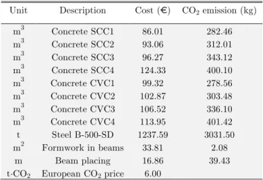
place-ment. The basic prices and emissions considered, given in Table 2, were obtained from the 2013 BEDEC ITEC database of the Institute of Construction Technology of Catalonia (BEDEC, 2013). Concrete unit price and CO2 emissions were determined from each mix design, including transport

and placing (García-Segura et al., 2014). Concerning the plasticizer used, CO2 emissions were those

given by the European Federation of Concrete Admixtures Associations, since it distinguishes be-tween plasticizer (EFCA, 2006a) and superplasticizer (EFCA, 2006b). It is considered that the silica fume does not produce emissions, since it is a waste product (García-Segura et al., 2014). Finally, the cost of CO2 emissions was that given in SENDECO2 (2013).

Table 2 Unit prices and emissions considered in the RC I-beam.

Unit Description Cost (€) CO2 emission (kg)

m3 Concrete SCC1 86.01 282.46

m3 Concrete CVC1 99.32 278.56

t Steel B-500-SD 1237.59 3031.50

m2 Formwork in beams 33.81 2.08

m Beam placing 16.86 39.43

(6)

Latin American Journal of Solids and Structures 11 (2014) 1190-1205 Carbonation captures CO2 and therefore, this capture should be subtracted from the embedded

CO2 emissions. This CO2 capture was estimated based on the predictive models of Fick’s First Law

of Diffusion (Collins, 2010; Lagerblad, 2005). Equation (5) estimates CO2 capture as the product of

the carbonation rate coefficient k, the structure service life t, the quantity of Portland cement per cubic meter of concrete c, the amount of CaO content in Portland cement (assumed to be 0.65), the proportion of calcium oxide that can be carbonated r (assumed to be 0.75 (Lagerblad, 2005)), the exposed surface area of concrete A, and the chemical molar fraction M (CO2/CaO is 0.79). The

quantity of Portland cement per cubic meter of concrete of every mixture is provided in Table 1.

M

A

r

CaO

c

t

k

CO

₌

_⋅

2 (5)

3 RESULTS

GSO was originally proposed by Krishnanand and Ghose (2009) to find solutions to the optimiza-tion of multiple optima continuous funcoptimiza-tions. GSO is a swarm intelligence algorithm based on the release of luciferin by glowworms. This luciferin attracts glowworms creating a movement toward another glowworm that is in its neighbourhood and glows brighter. The choice is encoded by a probabilistic function and the neighbourhood by a dynamic radial rate. The luciferin level depends on the fitness of its location, which is evaluated using the objective function.

GSO based algorithms present three main drawbacks: the glowworms may get stuck in local optima, they easily fall into an unfeasible solution and they have slow convergence rate. To over-come these problems, a hybridized method combining simulating annealing and glowworm swarm optimization (SAGSO) algorithms is proposed. Simulated annealing (SA) can escape from the local optima thanks to its probabilistic jumping property. Besides, SA accelerates convergence to the optimum.

Simulated annealing was originally proposed by Kirkpatrick et al. (1983) to design electronic circuits. This algorithm is based on the analogy of crystal formation from masses melted at high temperature and cooled slowly to allow atoms to align themselves reaching a minimum energy state. The probability of accepting new solutions is governed by the expression exp (-ΔE/T), where

ΔE is the increment in energy of the new configuration and T is the temperature. The initial tem-perature T0 is usually adjusted following methods like that proposed by Medina (2001). The initial

temperature is halved when the percentage of acceptances is greater than 40%, and the initial tem-perature is doubled if it is less than 20%. An exponential annealing schedule is adopted using a cooling rate k to control the temperature decrement once a Markov chain Mc ends. Hence, the

probability of accepting a worse solution drops with each Mc. The temperature decrement is given

by

T

_i

+1

=

kT

i (6)

where Ti and Ti+1 are the system temperatures at i and i+1 iteration. The minimum and maximum

(7)

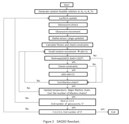
After a glowworm movement, SA updates the glowworm position with a local search strategy. Figure 2 shows a flowchart of the simulated process. The algorithm ends when the number of itera-tions t reaches the maximum tmax. The SAGSO algorithm is presented below.

1.A swarm of n feasible glowworms is randomly generated within the search space. To each glowworm, several parameters are assigned: initial luciferin value l0, initial radial sensor

range rs, and initial temperature T0. After assessing each glowworm objective function, the

worst objective value A is chosen.

2.The luciferin value is updated as the sum of the two terms, according to equation (7). The first term simulates the reduction in luciferin level with time, and the second term repre-sents the enhancement of the value of the objective function. As the algorithm must mini-mize both objective functions, the second term is modified. The difference between the worst objective value A and the value of the objective function at time t+1 is evaluated.

l

_i

(

t

₊

₁

)

₌

(

₁

₋

_ρ

)

_⋅

l

_i

( )

t

₊

_γ

(

A

₋

J x

(

_i

(

t

₊

₁

)

₍₇₎

where: li is the previous luciferin level; J(xi) is the objective function; ρ is the luciferin value

decay constant (0 < ρ < 1), and γ is the luciferin enhancement constant (0 < γ< 1).

3.The probability of moving toward a neighbour j is given by the equation (8), where

j

∈

N

_i

( )

t

,

N

i

( )

t

=

j

:

d

ij

<

r

d i

t

( )

;

l

i

( )

t

<

l

j

( )

t

{

}

. Ni(t) is the set of neighbours of the

glow-worm i at the iteration t. The neighbours must have higher luciferin value, they must be lo-cated within the radial sensor range

r

i

( )

t

d and they must be feasible solutions. Distance dij

represents the Euclidean distance between glowworms i and j.

p

_ij

( )

t

=

l

j

( )

t

−

l

i

( )

t

l

k

( )

t

−

l

i

( )

t

k∈N_i( )t

∑

(8)

4.Equation (9) defines the glowworm i movement toward the chosen glowworm j. Here, s (>0) is the step size. Although GSO was based on continuous variables, this algorithm adapts the new position to the closest discrete position thanks to the discrete nature of the struc-tural variables. This proposal was already assumed for the PSO algorithm (Parsopoulos and Vrahatis, 2002; He et al., 2004).

x

_i

(

t

+

1 )

₌

int

_x

i

( )

t

+

s

x

j

( )

t

−

x

i

( )

t

d

_ij

⎛

⎝⎜

⎞

⎠⎟

⎡

⎣

⎢

⎤

⎦

⎥

(9)

5.The radial sensor range is updated (6) according to equation (10), where: β is a constant pa-rameter, and nt is a parameter to control the number of neighbours. The new solution is

(8)

r

_di

(

t

₊

1 )

=

min

{

r

_s

,

max

⎡⎣

r

_di

( )

t

₊

β

(

n

_t

−

N

_i

( )

t

)

⎤⎦

}

₍10₎

6.A total nM Markov chains are run. The solution is modified by a small random movement; nv

variables are modified by a small random variation higher or lower to the values of these nv

variables.

7.The solution is evaluated. Only feasible solutions whose probability is greater than a random number between 0 to 1 are accepted.

random

<

e

J x( i( )t)−J x( i(t+1))

T (11)

8.When the Markov chain ends, the temperature decreases according to equation (6).

3 RESULTS USING SAGSO METHOD

In this section, we examine the results from computational experiments involving SAGSO optimiza-tion applied to a simply supported concrete I-Beam with a 15 m span, considering the parameters defined in section 2.1. The algorithm was coded in Intel® Visual Fortran Compiler Integration for Microsoft Visual Studio 2010 with a INTEL® CoreTM i7-3820 CPU processor with 3.6 GHz.

(9)

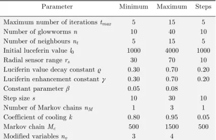
To define the SAGSO parameters (tmax, n, nt, l0, rs, ρ, γ, β, s, nM, k, Mc, nv), the algorithm was

run 3600 times. Each of the 400 combinations of parameters was performed nine times to obtain statistical data of the results. The parameters were randomly generated between their minimum and maximum values given in Table 3. Figure 3 shows the average cost and the computing time of each run. Tables 4 and 5, respectively, give the statistical results and the parameters of the best values when both cost and computing time are considered.

Table 3 Values of glowworm swarm parameters.

Parameter Minimum Maximum Steps

Maximum number of iterations tmax 5 15 5

Number of glowworms n 10 40 10

Number of neighbours nt 5 15 5

Initial luceferin value l0 1000 4000 1000

Radial sensor range rs 30 70 10

Luciferin value decay constant ρ 0.30 0.70 0.20 Luciferin enhancement constant γ 0.30 0.70 0.20

Constant parameter β 0.05 0.08

Step size s 10 30 10

Number of Markov chains nM 1 3 1

Coefficient of cooling k 0.80 0.95 0.05

Markov chain Mc 500 1500 500

Modified variables nv 3 4

(10)

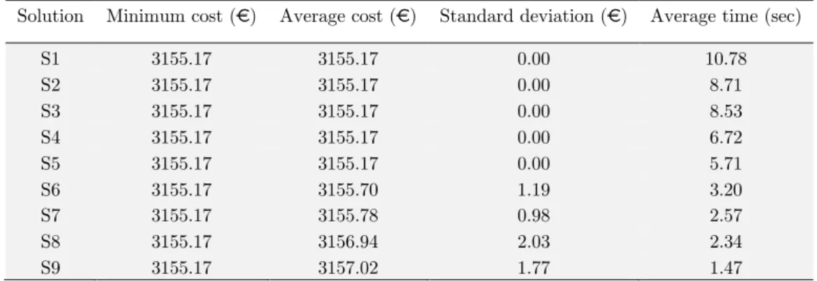
Latin American Journal of Solids and Structures 11 (2014) 1190-1205 Table 4 Statistical results of the best values for the minimum cost of SAGSO.

Solution Minimum cost (€) Average cost (€) Standard deviation (€) Average time (sec)

S1 3155.17 3155.17 0.00 10.78

S2 3155.17 3155.17 0.00 8.71

S3 3155.17 3155.17 0.00 8.53

S4 3155.17 3155.17 0.00 6.72

S5 3155.17 3155.17 0.00 5.71

S6 3155.17 3155.70 1.19 3.20

S7 3155.17 3155.78 0.98 2.57

S8 3155.17 3156.94 2.03 2.34

S9 3155.17 3157.02 1.77 1.47

Table 5 Parameters of the best values for the minimum cost of SAGSO.

Solution n nt l0 rs ρ γ β s nv Mc k tmax nM

S1 40 15 3000 40 0.50 0.30 0.05 10 3 1500 0.90 15 2 S2 40 5 2000 40 0.50 0.70 0.05 10 4 1500 0.90 10 3 S3 40 10 2000 40 0.70 0.70 0.05 20 3 1500 0.85 10 3 S4 20 5 1000 40 0.70 0.50 0.05 20 3 1500 0.90 15 3 S5 40 15 2000 60 0.50 0.50 0.05 20 3 1500 0.85 15 2 S6 20 10 1000 70 0.50 0.70 0.05 10 3 1500 0.80 10 2 S7 20 5 3000 60 0.70 0.50 0.05 10 3 1500 0.85 10 2 S8 10 15 2000 50 0.70 0.70 0.05 20 3 1500 0.85 10 3 S9 40 15 4000 60 0.70 0.70 0.05 10 3 500 0.80 15 1

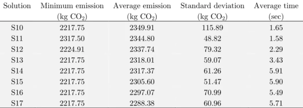
The same procedure was repeated again minimizing CO2 emissions. Figure 4 shows the average

CO2 emissions and the computing time. Concerning the best values for the average CO2 emissions

and minimum CO2 emissions, Table 6 summarizes the statistical results. The corresponding

param-eters are given in Table 7. Finding the global optimum was more difficult in this case. Besides, the standard deviation was higher.

(11)

Table 6 Statistical results of the best values for the minimum CO2 of SAGSO.

Solution Minimum emission (kg CO2)

Average emission (kg CO2)

Standard deviation (kg CO2)

Average time (sec)

S10 2217.75 2349.91 115.89 1.65

S11 2317.50 2344.80 48.82 1.58

S12 2224.91 2337.74 79.32 2.29

S13 2217.75 2318.01 59.07 3.43

S14 2217.75 2317.37 61.26 5.91

S15 2217.75 2305.60 51.47 5.90

S16 2217.75 2297.07 70.99 5.49

S17 2217.75 2288.38 60.96 5.71

Table 5 Parameters of the best values for the minimum CO2 of SAGSO.

Solution n nt l0 rs ρ γ β s nv Mc k tmax nM

S10 10 5 1000 40 0.70 0.30 0.05 30 3 1000 0.90 15 2 S11 10 5 2000 30 0.30 0.30 0.05 30 4 1000 0.85 15 2 S12 20 10 1000 30 0.70 0.30 0.05 20 4 1500 0.80 15 1 S13 20 15 4000 60 0.70 0.70 0.05 20 4 1500 0.80 10 2 S14 20 10 3000 30 0.70 0.50 0.05 20 3 1500 0.90 10 3 S15 40 10 2000 70 0.70 0.50 0.05 30 3 1000 0.90 15 2 S16 40 10 4000 60 0.70 0.70 0.05 30 4 500 0.90 15 2 S17 30 5 2000 30 0.70 0.70 0.05 30 4 1000 0.90 15 2

Comparing the cost-optimized beam with the emission-optimized beam (Table 8), it is worth noting that emission-optimized beam has a larger section, with a greater amount of concrete and less steel. The exposed surface area of the emission-optimized beam was nearly double, since the algorithm searched maximizing the CO2 capture. Concrete cover was 35mm, the maximum allowed.

Concerning the concrete mix, the cost-optimized beam acquired 54.2 MPa SCC and emission-optimized beam acquired 31.10 MPa CVC. The emission-emission-optimized beam achieved 26% fewer CO2

emissions, but this solution is 65% more expensive.

Table 8 Values of variables and constraints coefficients of the optimal design.

Variable Cost-optimized Emission-optimized

h (mm) 1570 2470

bfs (mm) 450 600

bfi (mm) 300 1000

tfs(mm) 150 150

tfi (mm) 170 150

tw (mm) 150 150

r (mm) 30 35

n1 10 17

n₂ 4 32

(12)

Latin American Journal of Solids and Structures 11 (2014) 1190-1205 Table 8 (continued) Values of variables and constraints coefficients of the optimal design.

n4 4 5

n5 9 6

Φ1 (mm) 6 6

Φ2 (mm) 25 8

Φ3 (mm) 25 8

Φ4 (mm) 8 6

Φ5 (mm) 6 6

Φ6 (mm) 6 6

Φ7 (mm) 6 6

Concrete SCC3 CVC1

Deflection coef.1 1.00 9.07

Cracking coef.1 1.52 infinite Cracking coef.2 3.03 infinite

Bending coef.1 1.08 1.00

Bending coef.2 1.36 1.52

Transversal shear coef.3 1.00 1.08 Transversal shear coef.2 1.55 1.37 Longitudinal superior shear coef. 1.64 1.59 Longitudinal inferior shear coef. 4.21 1.56 Amount of steel (kg) 383.14 353.57 Volume of concrete (m3) 4.54 8.44

Cost (€) 3155.17 5213.55

Emissions (kg CO2) 3017.14 2217.75 Service life (years) 169.71 221.84 1. Verification on central section

2. Verification on the boundary of two different sections

3. Verification on a section located an effective depth distance away from the edge of the sup-port

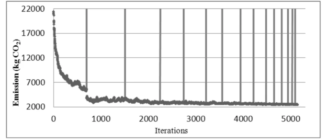
Figure 5 shows a typical curve for CO2 emissions following SAGSO. The optimization process

encompasses a SA search and a GSO movement (represented by a vertical line). While SA only makes small movements, GSO can jump to a quite different solution.

(13)

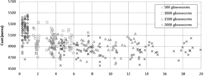
5 COMPARISON BETWEEN HEURISTICS

The proposed SAGSO algorithm is compared with the SA and GSO methods. Figure 6 shows the cost optimization results with GSO. The best solution obtained with GSO was 4557.84 euros with a computing time of 8.86 sec. Therefore, SAGSO found high quality solutions with the same compu-ting time. Concerning SA, the algorithm found the best cost-optimized and emission-optimized beam but the computer time increased 30 times.

SAGSO achieved the goal sought, which was to improve the exploitation of the algorithm. GSO provided the global searching capability and SA speeded up the local search. Its efficiency was well proven. A good calibration is needed to guarantee high quality solutions with a short computing time.

Figure 6 Average cost results of GSO.

6 CONCLUSIONS

In this paper, a hybrid method combining simulated annealing with glowworm swarm optimization (SAGSO) algorithms is presented and employed to optimize a concrete I-beam. The algorithm min-imizes the economic cost and CO2 emissions of a simply-supported concrete I-beam. The algorithm

is adapted to the discrete nature of the structural variables. The findings provide evidence to sug-gest that large sections with a highly exposed surface area and the use of CVC with the lower strength grade can minimize the CO2 emissions.

(14)

Acknowledgments This work was supported by the Spanish Ministry of Science and Innovation (Research Project BIA2011-23602) and by the Universitat Politècnica de València (Research Project PAID-06-12). The authors are also grateful to Dr. Debra Westall for her thorough revision of the manuscript.

References

Ahandania, M.A., Vakil-Baghmishehb, M.T., Zadehc, M.A.B., Ghaemic, S. (2012). Hybrid particle swarm opti-mization transplanted into a hyper-heuristic structure for solving examination timetabling problem. Swarm Evo-lutionary Computation 7:21-34.

Basturk, B., Karaboga, D. (2006). An Artificial Bee Colony (ABC) algorithm for numerical function optimiza-tion. IEEE Swarm Intelligence Symposium, Indianapolis, Indiana, USA.

BEDEC. (2013). Institute of Construction Technology of Catalonia. Barcelona, Spain.

Carbonell, A., Yepes, V., González-Vidosa, F. (2012). Automatic design of concrete vaults using iterated local search and extreme value estimation. Latin American Journal of Solids and Structures 9(6):675-689.

Chen, S., Sarosh, A., Dong, Y. (2012). Simulated annealing based artificial bee colony algorithm for global nu-merical optimization. Applied Mathematics and Computation 219(8):3575–3589.

Collins, F. (2010). Inclusion of carbonation during the life-cycle of built and recycled concrete: influence on their carbon footprint. The International Journal of Life Cycle Assessment 15(6):549-556.

Colorni, A., Dorigo, M., Maniezzo, V. (1991). Distributed optimization by ant colonies. Proceeding of ECAL-European Conference on Artificial Life, Elsevier, Paris, pp. 134-142.

Dutta, R., Ganguli, R., Mani, V. (2011). Swarm intelligence algorithms for integrated optimization of piezoelec-tric actuator and sensor placement and feedback gains. Smart Materials and Structures 20(10) 105018.

EFCA. (2006a). Environmental Product Declaration (EPD) for Normal Plasticising admixtures. Environmental Consultant, Sittard. http://www.efca.info/downloads/324%20ETG%20Plasticiser%20EPD.pdf, (acessed January 2013).

EFCA. (2006b). Environmental Product Declaration (EPD) for Superplasticising admixtures. Environmental Consultant, Sittard. http://www.efca.info/downloads/325%20ETG%20Superplasticiser%20EPD.pdf, (accessed January 2013).

Fan, S.K.S., Zahara, E. (2007). A hybrid simplex search and particle swarm optimization for unconstrained op-timization. European Journal of Operational Research 181(2):527–548.

Fomento, M. (2008). EHE: Code of structural concrete. Ministerio de Fomento, Madrid [in Spanish].

García-Segura, T., Yepes, V., Alcalá, J. (2014). Life-cycle greenhouse gas emissions of blended cement concrete including carbonation and durability. The International Journal of Life Cycle Assessment 19(1):3-12.

Gong, Q.Q., Zhou, Y.Q., Yang, Y. (2011). Artificial Glowworm Swarm Optimization Algorithm for Solving 0-1 Knapsack Problem. Advanced Materials Research 143-144:166-171.

Hare, W., Nutini, J., Tesfamariam, S. (2013). A survey of non-gradient optimization methods in structural engi-neering. Advances in Engineering Software 59:19-28.

He, S., Prempain, E., Wu, Q. (2004). An improved particle swarm optimizer for mechanical design optimization problems. Engineering Optimization 36(5):585–605.

Karaboga, D., Basturk, B. (2008). On the performance of Artificial Bee Colony (ABC). Applied Soft Computing 8(1):687-697.

(15)

Khan, K., Sahai, A. (2012). A Glowworm Optimization Method for the Design of Web Services. International Journal of Intelligent Systems and Applications 4(10):89-102.

Kicinger, R., Arciszewski, T., De Jong, K. (2005). Evolutionary computation and structural design: a survey of the state-of-the-art. Computers & Structures 83(23-24):1943-1978.

Kirkpatrick, S., Gelatt, C.D., Vecchi, M.P. (1983). Optimization by simulated annealing. Science 220(4598):671– 680.

Koide, R. M., de França, G.Z., Luersen, M.A. (2013). An ant colony algorithm applied to lay-up optimization of laminated composite plates. Latin American Journal of Solids and Structures 10(3):491-504.

Krishnanand, K.N., Ghose, D. (2009). Glowworm swarm optimization: a new method for optimizing multi-modal functions. International Journal of Computational Intelligence Studies 1(1):93-119.

Lagerblad, B. (2005). Carbon dioxide uptake during concrete life-cycle: State of the art. Swedish Cement and Concrete Research Institute, Stockholm, Sweden.

Li, L.J., Huang, Z.B., Liu, F. (2009). A heuristic particle swarm optimization method for truss structures with discrete variables. Computers & Structures 87(7-8):435-443.

Liao, W., Kao, Y., Li, Y. (2011). A sensor deployment approach using glowworm swarm optimization algorithm in wireless sensor networks. Expert Systems with Applications 38(10):12180-12188.

Luo, Q.F., Zhang, J.L. (2011). Hybrid Artificial Glowworm Swarm Optimization Algorithm for Solving Con-strained Engineering Problem. Advanced Materials Research 204-210:823-827.

Martí, J.V., González-Vidosa, F., Yepes, V., Alcalá, J. (2013). Design of prestressed concrete precast road bridges with hybrid simulated annealing. Engineering Structures 48:342-352.

Martínez-Martín, F., González-Vidosa, F., Hospitaler, A., Yepes, V. (2013). A parametric study of optimum tall piers for railway bridge viaducts. Structural Engineering and Mechanics 45(6):723-740.

Medina, J. (2001). Estimation of incident and reflected waves using simulated annealing. ASCE Journal of Wa-terway, Port, Coastal, and Ocean Engineering 127(4):213–221.

Parsopoulos, K., Vrahatis, M. (2002). Recent approaches to global optimization problems through particle swarm optimization. Natural Computing 1(2-3):235–306.

Payá-Zaforteza, I., Yepes, V., González-Vidosa, F., Hospitaler, A. (2010). On the Weibull cost estimation of building frames designed by simulated annealing. Meccanica 45(5):693-704.

Qu, L., He, D., Wu, J. (2011). Hybrid Coevolutionary Glowworm Swarm Optimization Algorithm with Simplex Search Method for System of Nonlinear Equations. Journal of Information & Computational Science 8(13):2693– 2701.

Sarma, K.C., Adeli, H. (1998). Cost optimization of concrete structures. ASCE Journal of Structural Engineering 124(5):570-578.

SENDECO2. (2013). http://www.sendeco2.com/es/precio_co2.asp?ssidi=1, (accessed January 2013).

Shieh, H.L., Kuo, C.C., Chiang, C.M. (2011). Modified particle swarm optimization algorithm with simulated annealing behavior and its numerical verification. Applied Mathematics and Computation 218(8):4365-4383. Sideris, K.K., Anagnostopoulos, N.S. (2013). Durability of normal strength self-compacting concretes and their impact on service life of reinforced concrete structures. Construction and Building Materials 41:491–497.

Torres-Machí, C., Yepes, V., Alcalá, J., Pellicer, E. (2013). Optimization of high-performance concrete structures by variable neighborhood search. International Journal of Civil Engineering 11(2):90-99.

Tuutti, K. (1982). Corrosion of steel in Concrete. CBI Forskning Research Report. Cement and Concrete Re-search Institute, Stockholm, Sweden.

(16)

Wang, H., Sun, H., Li, C., Rahnamayan, S., Pan, J. (2013). Diversity enhanced particle swarm optimization with neighborhood search. Information Sciences 223(20):119–135.

Yang, Y., Zhou, Y., Gong, Q. (2010). Hybrid Artificial Glowworm Swarm Optimization Algorithm for Solving System of Nonlinear Equations. Journal of Computational Information Systems 6(10):3431-3438.

Yepes, V., González-Vidosa, F., Alcalá, J., Villalba, P. (2012). CO2-Optimization design of reinforced concrete re-taining walls based on a VNS-threshold acceptance strategy. ASCE Journal of Computing in Civil Engineering 26(3):378-386.