www.atmos-chem-phys.net/16/15165/2016/ doi:10.5194/acp-16-15165-2016
© Author(s) 2016. CC Attribution 3.0 License.
Fluorescent bioaerosol particle, molecular tracer, and fungal spore
concentrations during dry and rainy periods in a semi-arid forest
Marie Ila Gosselin1,2, Chathurika M. Rathnayake3, Ian Crawford4, Christopher Pöhlker2,
Janine Fröhlich-Nowoisky2, Beatrice Schmer2, Viviane R. Després5, Guenter Engling6, Martin Gallagher4, Elizabeth Stone3, Ulrich Pöschl2, and J. Alex Huffman1
1Department of Chemistry and Biochemistry, University of Denver, Denver, CO, USA
2Max Planck Institute for Chemistry, Multiphase Chemistry and Biogeochemistry Departments, Mainz, Germany 3Department of Chemistry, University of Iowa, Iowa City, IA, USA
4Centre for Atmospheric Science, SEAES, University of Manchester, Manchester, UK 5Institute of General Botany, Johannes Gutenberg University, Mainz, Germany 6Division of Atmospheric Sciences, Desert Research Institute, Reno, NV, USA
Correspondence to:J. Alex Huffman (alex.huffman@du.edu)
Received: 16 August 2016 – Published in Atmos. Chem. Phys. Discuss.: 7 September 2016 Revised: 4 November 2016 – Accepted: 7 November 2016 – Published: 8 December 2016
Abstract.Bioaerosols pose risks to human health and agri-culture and may influence the evolution of mixed-phase clouds and the hydrological cycle on local and regional scales. The availability and reliability of methods and data on the abundance and properties of atmospheric bioaerosols, however, are rather limited. Here we analyze and com-pare data from different real-time ultraviolet laser/light-induced fluorescence (UV-LIF) instruments with results from a culture-based spore sampler and offline molecular trac-ers for airborne fungal spores in a semi-arid forest in the southern Rocky Mountains of Colorado. Commercial UV-APS (ultraviolet aerodynamic particle sizer) and WIBS-3 (wideband integrated bioaerosol sensor, version 3) instru-ments with different excitation and emission wavelengths were utilized to measure fluorescent aerosol particles (FAPs) during both dry weather conditions and periods heavily in-fluenced by rain. Seven molecular tracers of bioaerosols were quantified by analysis of total suspended particle (TSP) high-volume filter samples using a high-performance anion-exchange chromatography system with pulsed amperometric detection (HPAEC-PAD). From the same measurement cam-paign, Huffman et al. (2013) previously reported dramatic in-creases in total and fluorescent particle concentrations during and immediately after rainfall and also showed a strong rela-tionship between the concentrations of FAPs and ice nuclei (Huffman et al., 2013; Prenni et al., 2013). Here we
investi-gate molecular tracers and show that during rainy periods the atmospheric concentrations of arabitol (35.2±10.5 ng m−3)
and mannitol (44.9±13.8 ng m−3) were 3–4 times higher than during dry periods. During and after rain, the corre-lations between FAP and tracer mass concentrations were also significantly improved. Fungal spore number concen-trations on the order of 104m−3, accounting for 2–5 % of
1 Introduction
Primary biological aerosols particles (PBAPs) are of keen interest within the scientific community, partially because methods for their quantification and characterization are advancing rapidly (Huffman and Santarpia, 2017; Sodeau and O’Connor, 2016). The term PBAPs, or equivalently bioaerosols, generally comprises several classes of airborne biological particles including viruses, bacteria, fungal spores, pollen, and their fragments (Després et al., 2012; Fröhlich-Nowoisky et al., 2016). Fungal spores are of particular atmo-spheric interest because they can cause a variety of deleteri-ous health effects in humans, animals, and agriculture, and it has been shown that they can represent a significant frac-tion of total organic aerosol emissions (Deguillaume et al., 2008; Gilardoni et al., 2011; Madelin, 1994), especially in tropical regions (Elbert et al., 2007; Huffman et al., 2012; Pöschl et al., 2010; Zhang et al., 2010). Current estimates of the atmospheric concentration of fungal spores range from 100 to more than 104m−3 (Frankland and Gregory, 1973; Gregory and Sreeramulu, 1958; Heald and Spracklen, 2009; Hummel et al., 2015; Sesartic and Dallafior, 2011). Fungal spores may also impact the hydrological cycle as giant cloud condensation nuclei or as ice nuclei (Haga et al., 2013; Mor-ris et al., 2013; Sesartic et al., 2013). Additionally, several classes of bioaerosols and their constituent components, such as (1→3)-β-D-glucan and endotoxins, have been implicated in respiratory distress and allergies (Burger, 1990; Douwes et al., 2003; Laumbach and Kipen, 2005; Linneberg, 2011; Pöschl and Shiraiwa, 2015). For example, asthma and al-lergies have shown notable increases during thunderstorms due to elevated bioaerosol concentrations (Taylor and Jons-son, 2004) especially when attributed to fungal spores (Allitt, 2000; Dales et al., 2003).
Molecular tracers have long been utilized as a means of aerosol source tracking (Schauer et al., 1996; Simoneit and Mazurek, 1989; Simoneit et al., 2004). In recent years, anal-ysis of molecular tracers has been utilized for the quantifi-cation of PBAPs in atmospheric samples and has been com-pared, for example, with results from microscopy (Bauer et al., 2008a) and culture samples (Chow et al., 2015b; Wom-iloju et al., 2003). Three organic molecules have been pre-dominately utilized as unique tracers of fungal spores: er-gosterol, mannitol, and arabitol. The majority of atmospher-ically relevant fungal spores are released by active wet-discharge processes common in Ascomycota and Basidiomy-cota, meaning that the fungal organism actively ejects spores at a time most advantageous for the spore dispersal and ger-mination processes, often when relative humidity (RH) is high (Ingold, 1971). While there are several mechanisms of active spore emission (e.g., Buller’s drop (Buller, 1909) and osmotic pressure canons (Ingold, 1971)), they each involve the secretion of fluid containing hygroscopic compounds, such as arabitol, mannitol, potassium and chloride ions, as well as other solutes (Elbert et al., 2007), released near the
site of spore growth. When the spores are ejected, some of the fluid adheres to the spores and becomes aerosolized. Several of these secreted compounds are thought to enter the atmo-sphere linked uniquely with spore emission processes, and so these tracers have been used to estimate atmospheric con-centrations of fungal spores. Arabitol and mannitol are both sugar alcohols (polyols) that serve as energy stores for the spore (Feofilova, 2001). Arabitol is unique to fungal spores and lichen, while mannitol is present in fungal spores, lichen, algae, and higher plants (Lewis and Smith, 1967). Ergosterol is found within the cell membranes of fungal spores (Weete, 1973) and has been used as an ambient fungal spore tracer (Di Filippo et al., 2013; Miller and Young, 1997). Compar-ing the seasonal trends of arabitol and mannitol with ergos-terol, Burshtein et al. (2011) showed positive correlations be-tween arabitol or mannitol and ergosterol only in the spring and autumn, suggesting that the source of these polyols is unlikely to be solely fungal in origin or that the amount of each compound emitted varies considerably between species type and season. While ergosterol has been directly linked to fungal spores in the air, ergosterol is prone to photochem-ical degradation and is difficult to analyze and quantify di-rectly. Quantification of ergosterol typically requires chemi-cal derivatization by silylation before analysis via gas chro-matography (Axelsson et al., 1995; Burshtein et al., 2011; Lau et al., 2006). In contrast, analysis of sugar alcohols by ion chromatography involves fewer steps and has been suc-cessfully applied to monitor seasonal variations of atmo-spheric aerosol concentration at a number of sites (Bauer et al., 2008a; Caseiro et al., 2007; Yang et al., 2012; Yttri et al., 2011a; Zhang et al., 2010, 2015) including pg m−3
(picograms per cubic meter) levels in the Antarctic (Barbaro et al., 2015). By measuring spore count and tracer concen-tration in parallel at one urban and two suburban sites in Vienna, Austria, Bauer et al. (2008a) estimated the amount of each tracer per fungal spore emitted. Potassium ions have also been linked to emission of biogenic aerosol (Pöhlker et al., 2012b) and are co-emitted with fungal spores; however, application of potassium as a fungal tracer is uncommon because it is predominantly associated with biomass burn-ing (Andreae and Crutzen, 1997). Additionally, (1→3)-β -D-glucan (fungal spores and pollen) and endotoxins (gram-negative bacteria) have also been widely used to measure other bioaerosols (Andreae and Crutzen, 1997; Cheng et al., 2012; Rathnayake et al., 2016b; Stone and Clarke, 1992).
have been developed and are being utilized by the atmo-spheric community for bioaerosol detection. Thus far, the most widely applied LIF instruments for ambient PBAP de-tection have been the ultraviolet aerodynamic particle sizer (UV-APS; TSI Inc. Model 3314, St. Paul, MN, USA) and the wideband integrated bioaerosol sensor (WIBS; University of Hertfordshire, Hertfordshire, UK, now licensed to Droplet Measurement Technologies, Boulder, CO, USA). Both of these commercially available instruments can provide infor-mation in real-time about particle size and fluorescence prop-erties of supermicron atmospheric aerosols. Characterization and co-deployment of these instruments over the past 10 years has expanded the knowledge base regarding how to analyze and utilize the information provided from these in-struments (Crawford et al., 2015; Healy et al., 2014; Hernan-dez et al., 2016; Huffman et al., 2013; Perring et al., 2015; Pöhlker et al., 2012a, 2013; Ruske et al., 2016), though the interpretation of UV-LIF results from individual particles is complicated by interfering material that is not biological in nature (Gabey et al., 2010; Huffman et al., 2012; Lee et al., 2010; Saari et al., 2013; Toprak and Schnaiter, 2013).
Here we present analysis of atmospheric concentrations of arabitol and mannitol in relation to results from real-time, ambient particle measurements reported by UV-APS and WIBS. We interrogate these relationships as they pertain to rain conditions (rainfall and RH) that have previously been shown to increase the concentrations of fluorescent aerosols and ice nuclei (Crawford et al., 2014; Huffman et al., 2013; Prenni et al., 2013; Schumacher et al., 2013; Yue et al., 2016). Active wet discharge of ascospores and basidiospores has frequently been reported to correspond with increased RH (Elbert et al., 2007), and fungal spore concentration has also been shown to increase after rain events (e.g., Jones and Har-rison, 2004). Here we estimate airborne fungal concentra-tions in a semi-arid forest environment utilizing a combi-nation of real-time fluorescence methods, molecular fungal tracer methods, and direct-to-agar sampling and culturing as parallel surrogates for spore analysis. This study of ambient aerosol represents the first quantitative comparison of real-time aerosol UV-LIF instruments with molecular tracers or culturing.
2 Methods 2.1 Sampling site
Atmospheric sampling was conducted as a part of the BEACHON-RoMBAS (Bio–hydro–atmosphere interactions of Energy, Aerosols, Carbon, H2O, Organics, and
Nitro-gen – Rocky Mountain BioNitro-genic Aerosol Study) field cam-paign conducted at the Manitou Experimental Forest Ob-servatory (MEFO) located 48 km northwest of Colorado Springs, Colorado (39◦06′0′′N, 105◦5′03′′W; 2370 m ele-vation) (Ortega et al., 2014). The site is located in the
cen-tral Rocky Mountains and is representative of the semi-arid montane pine-forested regions of North America. Dur-ing BEACHON-RoMBAS, a large, international team of re-searchers conducted an intensive set of measurements from 20 July to 23 August 2011. A summary of results from the campaign are published in the BEACHON campaign spe-cial issue of Atmospheric Chemistry and Physics (http:// www.atmos-chem-phys.net/special_issue247.html). All the data reported here were gathered from instruments and sen-sors located within a < 100 m radius (Fig. 1).
2.2 Online fluorescent instruments
UV-APS and WIBS-3 (model 3; University of Hertford-shire) instruments were operated continuously as a part of the study, and particle data were integrated to 5 min aver-ages before further analysis. The UV-APS was operated un-der procedures defined in previous studies (Huffman et al., 2013; Schumacher et al., 2013). A total suspended particle (TSP) inlet head∼5.5 m above the ground, mounted above the roof of a climate-controlled, metal trailer, was used to sample aerosol directed towards the UV-APS. Bends and hor-izontal stretches in the 0.75 inch tubing were minimized to reduce losses of large particles (Huffman et al., 2013). The UV-APS detects particles between 0.5 and 20 µm and records aerodynamic particle diameter and integrated total fluores-cence (420–575 nm) after pulsed excitation by a 355 nm laser (Hairston et al., 1997). Both UV-APS and WIBS instru-ments report information about particle number concentra-tion, but it is instructive here to show results in particle mass for comparison between all techniques. Total particle num-ber size distributions (irrespective of fluorescence properties) obtained from the UV-APS and WIBS were converted to mass distributions assuming spherical particles of unit par-ticle mass density, unless otherwise stated, as a first approxi-mation. Total particle concentration values (in µg m−3)were obtained for each 5 min period by integrating over the size range 0.5–15 µm, and these mass concentration values were averaged over the length of the filter sampling periods. Un-certainty in mass concentration values reported here is influ-enced by assuming a single value for particle mass density and because of slight dissimilarities between size bins of the UV-APS and WIBS instruments at particle sizes above 10 µm that dominate particle mass.
10 m 50 m (1)
(2)
(5)
Site Layout
(1) UV-APS (2) High-volume sampler (3) LWS (leaf wetness) (4) Rain gauges (5) WIBS-3 Approx.
Scale
(4) (3)
l
Figure 1. Aerial overview of BEACHON-RoMBAS field site at the Manitou Experimental Forest Observatory located northwest of Colorado Springs, CO. Locations of all instruments and sensors dis-cussed here are marked and were located within a 50 m radius. Fig-ure adapted from Fig. 1a of Huffman et al. (2013).
320–400 nm and the other in a band at 410–650 nm. These excitation and emission wavelengths result in a total of three channels of detection:λex280 nm,λem320–400 nm (FL1 or
channel A);λex280 nm,λem 410–650 nm (FL2 or channel
B); and λex 370 nm, λem 410–650 nm (FL3 or channel C)
(Crawford et al., 2014). Individual particles are considered fluorescent here if they exceed fluorescent thresholds for any channel, as defined as the average of a “forced trigger” base-line plus 3 standard deviations (SD) of the basebase-line measure-ment (Gabey et al., 2010).
WIBS particle-type analysis is utilized to define types of particles that have specific spectral patterns. As defined by Perring et al. (2015), the three different fluorescent chan-nels (FL1, FL2, and FL3) can be combined to produce seven unique fluorescent categories. Observed fluorescence in channel FL1 alone, but without any detectable fluores-cence in channel FL2 or FL3, categorizes a particle as type A. Similarly, observed fluorescence in channels FL2 or FL3, but in no other channels, places a particle in the B or C cat-egories, respectively. Combinations of fluorescence in these channels, such as a particle that exhibits fluorescence in both FL1 and FL2, categorizes a particle as type AB and so on for a possible seven particle types as summarized in Fig. S1 in the Supplement.
As a separate tool for particle categorization, the Uni-versity of Manchester has recently developed and applied a hierarchical agglomerative cluster analysis tool for WIBS data, which they have previously applied to the BEACHON-RoMBAS campaign (Crawford et al., 2014, 2015; Robin-son et al., 2013). Here we utilize clusters derived from WIBS-3 data as described by Crawford et al. (2015). Clus-ter data presented here were analyzed with the open-source
Python package FastCluster (Müllner, 2013). Briefly, hierar-chical agglomerative cluster analysis was applied to the en-tire data set and each fluorescent particle was uniquely clus-tered into one of four groups. Cluster 1, assigned by Craw-ford et al. (2015) as fungal spores, displayed a 1.5–2 µm mode and a daily peak in the early morning that paralleled relative humidity (Schumacher et al., 2013). Clusters 2, 3, and 4 have strong, positive correlations with rainfall and ex-hibit size modes that peak at < 1.2 µm and were initially de-scribed by Crawford et al. (2014) as bacterial particles. Here we have summed clusters 2–4 to a single group referred to as ClBact, for simplicity when comparing with molecular
trac-ers. It should be noted that assignment of name and origin (e.g., fungal spores or bacteria) to clusters is approximate and does not imply naming accuracy or particle homogeneity. Each cluster likely contains an unknown fraction of contam-inating particles, but the clusters are beneficial to group par-ticles more selectively than using fluorescent intensity alone. For more details see Robinson et al. (2013) and Crawford et al. (2015).
The WIBS-3 utilized here has since been superseded by the WIBS-4 (Univ. Hertfordshire, UK) and WIBS-4A (Droplet Measurement Technologies, Boulder, CO, USA). One important difference between the models is that the op-tical chamber design and filters of the WIBS-4 models were updated to enhance the overall sensitivity of the instrument (Crawford et al., 2014). Additionally, slight differences in de-tector gain between models and individual units can impact the relative sensitivity of the fluorescence channels. This may result in differences in fluorescent channel intensity between instrument models, as will be discussed later.
2.3 High-volume sampler
Total suspended particle samples were collected for molec-ular tracer and molecmolec-ular genetic analyses using a high-volume sampler (Digitel DHA-80) drawing 1000 L min−1 through 15 cm glass fiber filters (Macherey-Nagel GmbH, Type MN 85/90, 406015, Düren, Germany) over a variety of sampling times ranging from 4 to 48 h (Supplement Ta-ble S1). The sampler was located < 50 m from each of the UV-LIF instruments described here, approximately between the WIBS-3 and UV-APS. Prior to sampling, all filters were baked at 500◦C for 12 h to remove DNA and organic con-taminants. Samples were stored in pre-baked aluminum bags after sampling at−20◦C for 1–30 days and then at−80◦C
2.4 Slit sampler
A direct-to-agar slit sampler (Microbiological Air Sampler STA-203, New Brunswick Scientific Co, Inc., Edison, NJ) was used to collect culturable airborne fungal spores. The sampler was placed ∼2 m above the ground on a wooden support surface with 5 cm×5 cm holes to allow airflow both up and down through the support structure. Sampled air was drawn over the 15 cm diameter sampling plate filled with growth media at a flow rate of 28 L min−1for sampling pe-riods of 20 to 40 min. Growth media (malt extract medium) was mixed with antibacterial agents (40 units streptomycin, Sigma Aldrich; 20 units ampicillin, Fisher Scientific) to sup-press bacterial colony growth. Plates were prepared several weeks in advance and stored in a refrigerator at ca. 4◦C until
used for sampling. Before each sampling period, all surfaces of the samplers were sterilized by wiping with isopropyl al-cohol. Handling and operational blanks were collected to ver-ify that no fungal colonies were being introduced by handling procedures. A total of 14 air samples were collected over 20 days and immediately moved to an incubator (Amerex In-struments, Incumax IC150R) set at 25◦C for 3 days prior to counting fungal colonies formed. Each colony, present as a growing dot on the agar surface, was assumed to have origi-nated as 1 colony-forming unit (CFU; i.e., fungal spore) de-posited onto the agar by impaction during sampling. The at-mospheric concentration of CFU per air volume was calcu-lated using the sampler airflow. Further discussion of meth-ods and initial results from the slit sampler were published by Huffman et al. (2013).
2.5 Offline filter analyses 2.5.1 Carbohydrate analysis
Approximately one-eighth of each frozen filter was cut for carbohydrate analysis using a sterile technique, meaning that scissors were cleaned and sterilized, and cutting was per-formed in a positive-pressure laminar flow hood. In order to precisely determine the fractional area of the filter to be ana-lyzed, filters were imaged from a fixed distance above using a camera and compared to a whole, intact filter. Using Im-ageJ software (Rasband, 1997), the area of each filter slice showing particulate matter (PM) deposit was referenced to a whole filter, and thereby the amount of each filter utilized could be determined. The total PM mass was not measured and so this technique allowed for an estimation of the frac-tion of each sample used for the analysis, which corresponds to the fraction of PM mass deposited. The uncertainty on the filter area fraction is estimated at 2 %, determined as the per-cent of variation in the area of the filter edge (no PM deposit) as compared to the total filter area.
Water-soluble carbohydrates were extracted from glass fiber filter samples and analyzed following the procedure de-scribed by Rathnayake et al. (2016a). A total of 36 samples
were analyzed along with field and lab blanks. All lab and field blanks fell below method detection limits. Extraction was performed by placing the filter slice into a centrifuge tube that had been pre-rinsed with Nanopure™ water (re-sistance > 18.2 Mcm−1; Barnstead EasyPure II, 7401). A volume of 8.0 mL of Nanopure™ water was added to the filter in the centrifuge tube to extract water-soluble carbo-hydrates. Samples were then exposed to rotary shaking for 10 min at 125 rpm, sonication for 30 min at 60 Hz (Branson 5510, Danbury, CT, USA), and rotary shaking for another 10 min. After shaking, the extracted solutions were filtered through a 0.45 µm polypropylene syringe filter (GE Health-care, UK) to remove insoluble particles, including disinte-grated filter pieces. One 1.5 mL aliquot of each extracted so-lution was analyzed for carbohydrates within 24 h of extrac-tion. A duplicate 1.5 mL aliquot was stored in a freezer and analyzed if necessary, due to lack of instrument response or invalid calibration check, within 7 days of extraction. Anal-ysis of carbohydrates was done using a high-performance anion-exchange chromatography system with pulsed amper-ometric detection (HPAEC-PAD; Dionex ICS 5000, Thermo Fisher, Sunnyvale, CA, USA). Details of the instrument spec-ifications and quality standards for carbohydrate determina-tion are available in Rathnayake et al. (2016a). Calibradetermina-tion curves for mannitol, levoglucosan, glucose (Sigma-Aldrich), arabitol, and erythritol (Alfa Aesar) were generated with 7 points each, ranging in aqueous concentration from 0.005 to 5 ppm. The method detection limits for mannitol, levoglu-cosan, glucose, arabitol, and erythritol were determined to be 2.3, 2.8, 1.6, 1.0, and 0.6 ppb, respectively, by measuring the instrument response to filter extracts (Rathnayake et al., 2016a). One filter each was spiked with 10 ppb of the five compounds, followed by one extraction per filter from which seven aliquots were each analyzed by the instrument. The variability (3 SD) of the measured response was taken as the method detection limit. All calibration curves were checked daily using a standard solution to ensure all concentration values were within 10 % of the known value. Failure to main-tain a valid curve resulted in recalibration of the instrument.
2.5.2 DNA analysis
re-moved. When sequences displayed > 97 % similarity, they were grouped into operational taxonomic units (OTUs). 2.5.3 Endotoxin and glucan analysis
Sample preparation for quantification of endotoxin and (1→3)-β-D-glucan included extraction of five punches (0.5 cm2 each) of the glass filters with 5.0 mL of pyrogen-free water (Associates of Cape Cod Inc., East Falmouth, MA, USA), utilizing an orbital shaker (300 rpm) at room temperature for 60 min, followed by centrifuging for 15 min (1000 rpm). A 0.5 mL aliquot of supernatant was submit-ted to a kinetic chromogenic limulus amebocyte lysate (Chromo-LAL) endotoxin assay (Associates of Cape Cod Inc., East Falmouth, MA, USA), using a ELx808IU (BioTek Instrument Inc., Winooski, VT, USA) incubating absorbance microplate reader. For (1→3)-β-D-glucan measurement, 0.5 mL of 3 N NaOH was added to the remaining 4.5 mL of extract and the mixture was agitated for 60 min. Subse-quently, the solution was neutralized to pH 6–8 by the ad-dition of 0.75 mL of 2 N HCl. After centrifuging for 15 min (1→3)-β-D-glucan concentration was determined in the su-pernatant using the Glucatell® LAL kinetic assay (Asso-ciates of Cape Cod, Inc., East Falmouth, MA, USA). The minimum detection limits (MDLs) and reproducibility were 0.046 endotoxin units (EU) m−3±6.4 % for endotoxin and 0.029 ng m−3±4.2 % for (1→3)-β-D-glucan, respectively. Laboratory and field blank samples were analyzed as well, with lab blank values being below detection limits, while field blank values were used to subtract background levels from sample data. More details about the bioassays can be found elsewhere (Chow et al., 2015a).
2.6 Meteorology and wetness sensors
Meteorological data were recorded by a variety of sensors lo-cated at the site. Precipitation was recorded by a laser optical disdrometer (PARticle SIze and VELocity sensor – “PAR-SIVEL”; OTT Hydromet GmbH, Kempton, Germany) and separately by a tipping-bucket rain gauge. The disdrome-ter provides precipitation occurrence, rate, and physical state (rain or hail) by measuring the magnitude and duration of dis-ruption to a continuous 780 nm laser that was located in a tree clearing (Fig. 1), while the tipping-bucket rain gauge mea-sures a set amount of precipitation before tipping and trigger-ing an electrical pulse. A leaf wetness sensor (LWS; Decagon Devices, Inc., Pullman, WA, USA) provided a measurement of condensed moisture by measuring the voltage drop across a leaf surface to determine a proportional amount of water on or near the sensor. Additional details of these measure-ments can be found in Huffman et al. (2013) and Ortega et al. (2014).
3 Results and discussion
3.1 Categorization and characteristic differences of Dry and Rainy periods
Increases in PBAP concentration have been frequently as-sociated with rainfall (e.g., Bigg et al., 2015; Faulwetter, 1917; Hirst and Stedman, 1963; Jones and Harrison, 2004; Madden, 1997). Fungal polyols have also been reported to increase after rain and have been used as indicators of in-creased fungal spore release (Liang et al., 2013; Lin and Li, 2000; Zhu et al., 2015). Recently, it was shown that the con-centration of fluorescent aerosol particles (FAPs) measured during BEACHON-RoMBAS increased dramatically during and after periods of rain (Crawford et al., 2014; Huffman et al., 2013; Schumacher et al., 2013) and that these parti-cles were associated with high concentrations of ice nucle-ating particles that could influence the formation and evolu-tion of mixed-phase clouds (Huffman et al., 2013; Prenni et al., 2013; Tobo et al., 2013). It was observed that a mode of smaller fluorescent particles (2–3 µm) appeared during rain episodes, and several hours after rain ceased a second mode of slightly larger fluorescent particles (4–6 µm) emerged, per-sisting for up to 12 h (Huffman et al., 2013). The first mode was hypothesized to result from mechanical ejection of parti-cles due to rain splash on soil and vegetated surfaces, and the second mode was suggested as actively emitted fungal spores (Huffman et al., 2013). While the UV-APS and WIBS each provide data at a high enough time resolution to see subtle changes in aerosol concentration, the temporal resolution of the chemical tracer analysis was limited to 4–48 h periods de-fined by the collection time of the high-volume sampler. To compare the measurement results across the sampling plat-forms, UV-LIF measurements were averaged to the lower time resolution of the filter sampler periods, and the periods were grouped into three broad categories: Rainy, Dry, and Other, as will be defined below.
rain-1.0
0.8
0.6
0.4
0.2
0.0
Particle-type fraction
1.0 0.0
Rain (mm)
100
0
RH (%)
500 250
Wetness (mV)
40 30 20 10 0
10
3
spores (m
-3
)
1
2 4
10
2
Diameter (um)
7/25 7/25
8/1 8/1
8/8 8/8
8/15 8/15
8/22 8/22
Date (2011)
ABC BC AC AB C B A
Dry Rainy Other
RH Rainfall Leaf wetness
Arabitol Mannitol Cluster 1 (a)
(b)
(c)
(d)
(e)
0.15 0.10 0.05 0.00
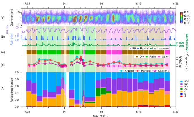
Figure 2.Time series of key species concentrations and meteorological data over entire campaign.(a)Fluorescent particle number size distribution measured with UV-APS instrument. Color scale indicates fluorescent particle number concentration (L−1).(b)Meteorological data: relative humidity (RH), disdrometer rainfall (millimeters per 15 min), leaf wetness (mV).(c)Wetness category indicated as colored bars: green, Rainy; brown, Dry; pink, Other. Bar width corresponds to filter sampling periods. Lightened colored bars extend vertically to highlight categorization.(d)Colored traces show fungal spore concentrations estimated from molecular tracers (circles) and WIBS Cl1 data (squares).(e)Stacked bars show relative fraction of fluorescent particle type corresponding to each WIBS category.
fall rate because it was observed that often only one of the two systems would record a given light rain event. If a point was described by total rainfall accumulation greater than 0.201 it was flagged as rain. A point was flagged as post-rain if it immediately followed a rain period and also exhibited a fluorescent particle fraction greater than 0.08. The purpose of this category was to reflect the observation that sustained el-evated concentrations of FAPs persisted for many hours even after the rain rate, RH, and leaf wetness returned to pre-rain values. The only measurement that adequately reflected this scenario was of the fluorescent particles measured by UV-APS and WIBS instruments. The post-rain flag was contin-ued until the fluorescent particle fraction fell below 0.08 or if it started to rain again (with calculated rain values greater than 0.201). Points were flagged as dry periods if they ex-hibited rainfall accumulation and fluorescent particle fraction below the thresholds stated above. Several periods were not easily categorized by this system and were considered in a fourth category as other. This occurred when fluorescent par-ticle fraction above the threshold value was observed with no discernable rainfall.
Once wetness categories were assigned by the algorithm at 15 min resolution, each high-volume filter sample was egorized by a similar nomenclature, but using only three
Rainy, presented a FAP fraction marginally above the 0.08 threshold, but visually displayed a trend dissimilar to other post-rain periods and so was re-categorized as Dry. Sample 28 showed no obvious rainfall, but the measurement team observed persistent fog in three consecutive mornings (sam-ples 25, 27, 28), and the concentration of fluorescent particles (2–6 µm) suggested a source of particles not influenced by rain, and so this Rainy sample was re-categorized as Other. Sample 38 displayed a fluorescent number ratio just below the threshold value, and was first categorized as Dry; how-ever, the measurement team observed post-rain periods at the beginning and end of the sample, and the sample was re-categorized as Other. For all samples other than these five, the categorization was determined using the majority (> 0.50) of the 15 min periods. In no cases other than the five that were re-categorized was the highest category fraction less than 0.50 of the sample time. Note that we have chosen to capitalize Rainy, Dry, and Other to highlight that we have rig-orously defined the period using the characterization scheme described above and to separate the nomenclature from the general, colloquial usage of the terms. Wetness category as-signment for each high-volume filter sample period is shown in Fig. 2 as a background color (brown for Dry samples, green for Rainy samples, and pink for Other samples) and Table S1.
To validate the qualitative differences between wetness categories described in the last section, we present observa-tions about each of these groupings. First, we organized the WIBS data according to the particle categories introduced by Perring et al. (2015). By this method, every fluorescent par-ticle detected by the WIBS can be defined uniquely into one of seven categories (i.e., A, AB, ABC). By plotting the rela-tive fraction of fluorescent particles described by each parti-cle type, temporal differences between measurement periods can be observed, as shown in Fig. 2e. To a first approxima-tion, this analysis style allows for coarse discrimination of particle types. For example, a given population of particles would ideally exhibit a consistent fraction of particles present in the different particle categories as a function of time. By this reasoning, sample periods categorized as Dry (most of the latter half of the study; brown bars in Fig. 2) would be ex-pected to have a self-consistent particle-type trend, whereas sample periods categorized as Rainy (most of the first half of the study; green bars in Fig. 2) would have a self-consistent particle-type trend, but different from the Dry samples. This is broadly true. During Rainy periods, as seen in Fig. 3a, there is a relatively high fraction (> 65 %) of ABC type par-ticles (light blue) and a relatively low fraction (< 15 %) in BC (purple) and C (yellow) type particles, suggesting heavy influence from the FL1 channel. In contrast, during Dry pe-riods the fraction of ABC particles (light blue) is reduced (< 25 %), whereas BC (purple) and C (yellow) type particles increase in relative fraction (> 30 and > 40 %, respectively), which suggested a diminished influence of FL1 channel.
Dry Rainy Other
Dry 1.2
0.8
0.4
0.0
Particle-type
fraction
1.0
0.8
0.6
0.4
0.2
0.0
OTU-relative
fraction
(a)
(b)
ABC BC AC AB C B A
Cystobasidiomycetes Lecanoromycetes Microbotryomycetes Pezizomycetes Ustilaginomycetes Eurotiomycetes Chytridiomycota Other fungi Leotiomycetes Tremellomycetes Sordariomycetes Other basidiomycota Other ascomycota Pucciniomycetes Dothideomycetes
148
49
106
39 10
17
37 Rainy
211 OTUs
Dry 246 OTUs
Other 103 OTUs (c)
Figure 3.Characteristic differences between wetness periods (Dry, Rainy, Other).(a)Relative fraction of fluorescent particle number corresponding to each WIBS category. Bars show relative standard deviation of category fraction in each wetness group (Dry, 19 sam-ples; Rainy, 11 samsam-ples; Other, 6 samples).(b, c)Distribution of fungal OTU (operational taxonomic unit) values.(b)Fungal com-munity composition at phylum and class level with Agaricomycetes (dominant class with consistently∼60 % of diversity) removed. Relative proportion of OTUs assigned to different fungal classes and phyla for each sample category shown.(c)Venn diagram show-ing the number of unique (wetness category-specific) and shared OTUs (represented by numbers in overlapping areas) among the sample categories (Dry, 11 samples; Rainy, 7 samples; Other, 3 sam-ples). OTUs classified as cluster of sequences with≥97 % similar-ity. Taxonomic assignments were performed using BLAST against NCBI database. In total, 3902 sequences, representing 406 fungal OTUs from 3 phyla and 12 classes were detected. Despite differ-ences in community structure across the sample categories, phylo-genetic representation appears largely similar.
frac-103 2 4
104
2 4
105
2 4
106
FAPs (m
-3 )
FL1 FL2 FL3 UV-APS
150
100
50
0
WIBS FL1 (10
3 m -3 )
500 400 300 200 100 0
UV-APS (103m-3)
500
400
300
200
100
0
WIBS FL2 (10
3 m -3 )
500 400 300 200 100 0
UV-APS (103m-3)
800
600
400
200
0
WIBS FL3 (10
3 m -3 )
500 400 300 200 100 0
UV-APS (103m-3)
(a) (b)
(c) (d)
Dry R2 = 0.80
Rainy R2 = 0.62
Other R2 = 0.86 Dry R2 = 0.82
Rainy R2 = 0.70
Other R2 = 0.92
Dry R2 = 0.20
Rainy R2 = 0.11
Other R2 = 0.17
Figure 4.Number concentration of fluorescent particles as a function of instrument channel, averaged over entire measurement period.(a) Box-and-whisker plot of fluorescent particle number concentration for WIBS FL1, FL2, FL3, and UVAPS. Circle markers shows mean values, internal gray horizontal line shows median, top and bottom of box show inner quartile, and whiskers show 5th and 95th percentiles. (b)WIBS FL1 vs. UV-APS,(c)WIBS FL2 vs. UV-APS, and(d)WIBS FL3 vs. UV-APS. Crosses represent 5 min average points. Linear fits assigned for data in each wetness category.
tion of particle categories for samples aerosolized in the lab. They reported fungal spores to be predominately A, AB, and ABC type particles, whereas Rainy sample periods, sug-gested to have a heavy fungal spore influence by Huffman et al. (2013), show predominantly C, BC, and ABC type parti-cle fractions. These discrepancies may be due to the compar-ison of ambient particles to laboratory-grown cultures. The highly controlled environment of a laboratory may not al-ways accurately represent the humidity conditions in which fungal spore release occurs in this forest setting (Saari et al., 2015). This could impact the fluorescence properties of fun-gal spore particles that have different amounts of adsorbed or associated water (Hill et al., 2009, 2013, 2015). More likely, however, is that the WIBS-3 used here exhibits differences in fluorescence sensitivity from the WIBS-4A used by Her-nandez et al. (2016). Even a slight increase in sensitivity in the FL3 channel with respect to the FL1 or FL2 channels could explain the shift here towards particles with C-type fluorescence. One piece of evidence for this is the quanti-tative comparison of particle measurements presented by the UV-APS and WIBS-3 instruments co-deployed here (Fig. 4). The number concentration of particles exhibiting fluores-cence above the FL2 baseline of the WIBS-3 is approxi-mately consistent with the number of fluorescent particles measured by the UV-APS, and significantly below the con-centration of FL3 particles. The UV-APS number concen-tration shows the highest correlation with the WIBS-3 FL2 channel: during Rainy periods,R2=0.70; Dry,R2=0.82;
and Other,R2=0.92. These observations are in stark con-trast to the trends reported by Healy et al. (2014) that the UV-APS fluorescent particle concentration correlated most strongly with the WIBS-4 FL3 and that the number concen-tration of FL3 was the lowest out of all three channels. Given that the FL3 channel of the WIBS and the UV-APS cover similar excitation and emission wavelengths, it is expected that these two channels should correlate well. Based on these data, we suggest that the WIBS-3 utilized here may present a very different particle-type breakdown than if a WIBS-4 had been used. So, while caution is recommended when com-paring the relative breakdown of WIBS particle categories shown here (Fig. 3) with other studies, the data are inter-nally self-consistent, and comparing qualitative differences between, e.g., Rainy and Dry periods, is expected to be ro-bust. The main point to be highlighted here is that there is in-deed a qualitative difference in particles present in the three wetness categories, as averaged and shown in Fig. 3a, which generally supports the effort to segregate these samples.
50
40
30
20
10
0
Arabitol
(ng m
)
–3
50
40
30
20
10
0
80
60
40
20
0
3.0 2.0 1.0 0.0
UV-APS FAP (µg m )–3
80
60
40
20
0
1.5 1.0 0.5 0.0
WIBS Cl1 FAP ( g m )µ –3 50
40
30
20
10
0
80
60
40
20
0
Mannitol
(ng m
)
–3
Dry y = 2.0x + 8.1
R2 = 0.13
Rainy y = 38.0x - 21.8 R2 = 0.73
Dry y=18.8x+6.9
R2=0.76
Rainy y=41.6x+14.6 R2=0.8 Dry
y=2.9x+8.3
R2=0.16
Rainy y=54.9x-37.5 R2=0.88
Dry y=9.9x+9.2
R2=0.11
Rainy y=32.0x+11.9 R2=0.82
(a) (c) (e)
(b) (d) (f)
Dry Rainy Other
Figure 5.Mass concentrations of molecular tracers and fluorescent particles (calculated assuming unit density particle mass and spherical particles): arabitol – top row and mannitol – bottom row. Average mass concentration of arabitol(a)and mannitol(b)in each wetness category. Central marker shows mean value of individual filter concentration values, bars represent standard deviation (SD) range of filter values, and individual points show outliers beyond mean±SD. Correlation of arabitol(c)and mannitol(d)with fluorescent particle mass from UV-APS. Correlation of arabitol(e)and mannitol(f)with fluorescent particle mass from WIBS cluster 1.R2values shown for each fit in(c–f). Linear fit parameters are shown in Table S2.
number of OTUs observed uniquely in either the Rainy or Dry periods is greater than the number of OTUs present in both wetness types, suggesting that the fungal communi-ties in each grouping are relatively distinct. Further, Fig. 3b shows a breakdown of fungal taxonomic groupings for each wetness group. This analysis shows that there is a qualita-tive difference in taxonomic breakdown between periods of Rainy and Dry. Specifically, during Dry periods there is an increased fraction of Pucciniomycetes (green bar, Fig. 3c), Chytridiomycota (yellow), Sordariomycetes (orange), and Eurotiomycetes (pink) when compared to the Rainy periods.
3.2 Atmospheric mass concentration of arabitol, mannitol, and fungal spores
To estimate fungal spore emission to the atmosphere, the concentration of arabitol and mannitol (Fig. 5a, b, Ta-ble 1) in each aerosol sample was averaged for all sam-ples in each of the three wetness categories. The average concentration of arabitol collected on Rainy TSP samples (35.2±10.5 ng m−3) increased by a factor of 3.3 with re-spect to Dry samples, and the average mannitol concen-tration on Rainy samples was higher by a factor of 3.7 (44.9±13.8 ng m−3). Figure 5a, b show the concentration
variability for each wetness category, observed as the stan-dard deviation from the distribution of individual samples. For each polyol, there is no overlap in the ranges shown, including the outliers of the Rainy and Dry category, sug-gesting a definitive and conceptually distinct separation be-tween dry periods and those influenced by rain. The concen-trations observed during Other periods is between those of the Dry and Rainy averages, as expected, given the difficulty
in confidently assigning these uniquely to one of these cat-egories. The observations here are roughly consistent with previous reports of polyol concentration, despite differences in local fungal communities and concentrations. For exam-ple, Rathnayake et al. (2016a) observed 30.2 ng m−3 ara-bitol and 41.3 ng m−3 mannitol in PM10 samples collected
in rural Iowa, USA. In addition, Zhang et al. (2015) re-ported arabitol and mannitol concentrations in PM10
sam-ples of 44.0 and 71.0 ng m−3, respectively, from a study in the mountains on Hainan Island off the coast of southern China. More recently, Yue et al. (2016) studied a rain event in Beijing and observed increased polyol concentrations at the onset of the rain. The observed mannitol concentration (45 ng m−3)was approximately consistent with observations reported here and with previous reports, while the arabitol concentration values observed were approximately an order of magnitude lower (0.3 ng m−3).
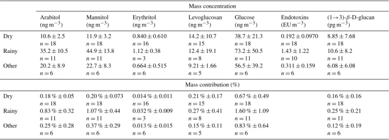
endo-Table 1. Campaign-average concentrations of molecular tracers (top) and their respective mass contributions (bottom). Values are mean±standard deviation;nshows number of samples used for averaging. Total particulate matter mass calculated from UV-APS num-ber concentration (m−3), converted to mass over aerodynamic particle diameter range 0.5–15 µm using 1.5 g cm−3density.
Mass concentration Arabitol
(ng m−3)
Mannitol (ng m−3)
Erythritol (ng m−3)
Levoglucosan (ng m−3)
Glucose (ng m−3)
Endotoxins (EU m−3)
(1→3)-β-D-glucan (pg m−3)
Dry 10.6±2.5
n=18
11.9±3.2
n=18
0.840±0.610
n=16
14.2±10.7
n=15
38.7±21.3
n=18
0.192±0.0970
n=18
8.85±7.68
n=18 Rainy 35.2±10.5
n=11
44.9±13.8
n=11
1.12±0.38
n=3
12.4±19.1
n=8
73.2±50.5
n=11
1.43±1.22
n=10
10.6±8.2
n=11 Other 20.2±8.9
n=6
22.7±8.3
n=6
0.664±0.515
n=6
9.21±1.66
n=5
56.5±39.2
n=6
0.311±0.159
n=6
6.08±6.08
n=6 Mass contribution (%)
Dry 0.18 %±0.05
n=18
0.20 %±0.073
n=18
0.014 %±0.011
n=16
0.21 %±0.17
n=15
0.67 %±0.49
n=18
0.16 %±0.16
n=18 Rainy 0.83 %±0.32
n=11
1.07 %±0.44
n=11
0.032 %±0.009
n=3
0.27 %±0.41
n=8
1.60 %±1.09
n=11
0.25 %±0.21
n=11 Other 0.25 %±0.28
n=6
0.37 %±0.29
n=6
0.013 %±0.015
n=6
0.15 %±0.11
n=5
0.83 %±0.64
n=6
0.12 %±0.19
n=6
Table 2.Square of correlation coefficients (R2)comparing total mass concentration of molecular tracers to each other. EU: endotoxin units. Boxes colored by coefficient value (bold> 0.7; 0.7 >italic> 0.4).
Arabitol Mannitol (1→3)-β-D-glucan
Rainy Dry Rainy Dry Rainy Dry
Mannitol Rainy 0.839
Dry 0.312
(1→3)-β-D-glucan Rainy 0.000 0.003
Dry 0.000 0.327
Endotoxins Rainy 0.116 0.126 0.427
Dry 0.012 0.113 0.103
toxins and glucans analyzed were not emitted uniquely from the same sources as arabitol and mannitol.
Results from the two UV-LIF instruments were averaged over high-volume sample periods, and a correlation analy-sis was performed between tracer mass and fluorescent parti-cle mass showing positive correlations in all cases. The FAP mass from the UV-APS shows high correlation with the fun-gal polyols during Rainy periods, withR2of 0.732 and 0.877 for arabitol and mannitol, respectively (Table 3; Fig. 5c, d). The same tracers correlate poorly with the UV-APS during Dry conditions. This is expected, because Ascomycota and Basidiomycota spores emitted by wet-discharge methods are the only fungal spores reported to be associated with arabitol and mannitol (Elbert et al., 2007; Feofilova, 2001; Lewis and Smith, 1967). This high correlation suggests that the UV-APS does a good job of detecting these wet-discharge spores, and corroborates previous statements that particles detected in ambient air by the UV-APS are often predominately fun-gal spores (Healy et al., 2014; Huffman et al., 2012, 2013).
In contrast, the low slope value and the poor correlation dur-ing Dry periods suggest that the UV-APS is also sensitive to other kinds of particles, as designed. The small positivex
offset (FAP mass; Table S2, Fig. 5c, d) during Rainy periods is likely due to particles that are too weakly fluorescent to be detected and counted by the UV-APS, which is consistent with observations made in Brazil (Huffman et al., 2012).
Table 3.Square of correlation coefficients (R2)comparing fluorescent particle measurements from UV-LIF instruments to measurements from molecular tracers and direct-to-agar sampler. Columns marking tracer mass indicate correlations between time-averaged UV-LIF and tracer mass concentrations (left side). Columns marking fungal spore count indicate correlations between fungal spore number concentrations estimated from time-averaged UV-LIF and tracer or culture measurements (right side). FL1, FL2, FL3 represent individual channels from the WIBS. FL represents particles exhibiting fluorescence in any channel. Cl1, Cl2, Cl3, Cl4 are clusters that estimate particle concentrations as a mixture of various channels (Crawford et al., 2015). ClBactis a sum of the “bacteria” clusters Cl2-4. Boxes colored by coefficient value (bold> 0.7; 0.7 >italic> 0.4).
Correlation based on tracer mass Correlation based on spore counts Arabitol Mannitol (1→3)-β-D-glucan Endotoxins Arabitol Mannitol CFU
Rainy Dry Rainy Dry Rainy Dry Rainy Dry Rainy Dry Rainy Dry Rainy Dry
UV
-LIF
mass
or
number
concentration
UVAPS 0.732 0.127 0.877 0.160 0.006 0.012 0.153 0.067 0.483 0.278 0.504 0.571 0.469 0.491
WIBS
FL 0.554 0.250 0.810 0.255 0.128 0.010 0.068 0.066 0.159 0.200 0.088 0.314 0.330 0.737
FL1 0.602 0.445 0.819 0.412 0.042 0.001 0.090 0.012 0.667 0.339 0.863 0.621 0.470 0.546
FL2 0.617 0.248 0.843 0.342 0.092 0.001 0.039 0.094 0.485 0.302 0.442 0.340 0.560 0.543
FL3 0.561 0.222 0.818 0.251 0.124 0.008 0.071 0.065 0.178 0.181 0.104 0.306 0.367 0.736
Cl1 0.824 0.764 0.799 0.109 0.000 0.134 0.229 0.011 0.679 0.543 0.775 0.423 0.128 0.690
Cl2 0.005 0.002 0.004 0.006 0.002 0.047 0.006 0.017 0.052 0.056 0.001 0.075 0.081 0.930
Cl3 0.267 0.164 0.261 0.198 0.003 0.011 0.016 0.066 0.052 0.116 0.087 0.439 0.262 0.383 Cl4 0.048 0.046 0.172 0.118 0.115 0.011 0.179 0.145 0.062 0.089 0.001 0.065 0.120 0.000
ClBact 0.041 0.081
of selecting fungal spore particles. The poor correlation be-tween mannitol and Cl1 during dry periods illustrates that the background mannitol concentration is likely not due to fungal spores alone, but has contributions from other higher plants that contain mannitol. Particle concentrations detected by individual WIBS channels and in the other clusters were also compared with polyol concentrations, but each correla-tion is relatively poor compared to that with respect to Cl1. As seen in Table 3 and Figs. S2–S3, correlations in FL1, 2, and 3 with arabitol are poor (< 0.4) in the Dry category and good (0.4 <R2 < 0.7) in the Rainy category. For mannitol, all the UV-LIF instruments show high correlation (> 0.7) in all cases. This is likely due to mannitol being a non-specific tracer and suggests that the majority of UV-LIF particles ob-served during all periods was dominated by PBAPs.
3.3 Estimated number concentration of fungal spore aerosol
Bauer et al. (2008a) reported measurements of fungal spore number concentration in Vienna, Austria, using epifluores-cence microscopy, and also measured fungal tracer mass col-lected onto filters in order to estimate the mass of arabitol (1.2 to 2.4 pg spore−1)and mannitol (0.8 to 1.8 pg spore−1)
associated with each emitted spore. Bauer et al. (2008a) and Yttri et al. (2011b) reported ratios of mannitol to arabitol of ca. 1.5 (±standard deviation of 26 %) and 1.4±0.3, respec-tively. Our measurements show slightly lower ratios of man-nitol to arabitol, but that the ratio is dependent on wetness category: Rainy, 1.29±0.17; Dry, 1.12±0.23; and Other, 1.24±0.54. The mannitol to arabitol ratio would be expected to vary as a function of fungal population present in the
aerosol, whether between different wetness periods at a given location or between different physical localities.
Using the approximate mid-point of the Bauer et al. (2008a) reported ranges, 1.7 pg mannitol per spore and 1.2 pg arabitol per spore, atmospheric number concentrations of spores collected onto the high-volume filters were calcu-lated from the polyol mass concentrations measured here. Based on these values, and assuming all polyol mass orig-inated with spore release, the mass concentration averages (Fig. 5) were converted to fungal spore number concentra-tions (Fig. 6). The trends of spore concentration averages are the same as with the polyol mass, because the numbers were each multiplied by the same scalar value. After doing so, the analysis reveals an estimated spore concentration dur-ing Dry periods of 0.89×10⁴(±0.21) spores m−3using the
arabitol concentration and 0.70×10⁴(±0.19) spores m−3
us-ing the mannitol concentration (Table 4). The estimated con-centration of spores increased approximately 3-fold during Rainy periods to 2.9×10⁴(±0.8) spores m−3(arabitol esti-mate) and 2.6×10⁴(±0.8) spores m−3(mannitol estimate) (Fig. 6a, b). These estimates match reasonably well with esti-mates reported by Spracklen and Heald (2014), who modeled the concentration of airborne fungal spores across the globe as an average of 2.5×10⁴ spores m−3, with ca. 0.5×10⁴ spores m−3over Colorado.
4
3
2
1
0
4
-3
4
3
2
1
0
4
3
2
1
0
4
3
2
1
0 4
3
2
1
0
4
3
2
1
0
Fungal
spores
(10
m
)
Fungal
spores
(10
m
)
4
-3
Rainy R2=0.48
Dry R2=0.28
Rainy R2=0.78
Dry R2=0.42
Rainy R2 = 0.5
Dry R2=0.57
Rainy R2=0.68
Dry R2=0.54
Dry Rainy Other
(a) (d) (g)
(b) (e) (h)
1.0
0.8
0.6
0.4
0.2
0.0
4 3 2 1 0
WIBS Cl1 FAPs (104m-3)
1.0
0.8
0.6
0.4
0.2
0.0
Colony-forming
units
(10
m
)
3
-3
12 10 8 6 4 2 0
UV-APS FAPs (104m-3)
1.0
0.8
0.6
0.4
0.2
0.0
Rainy R2=0.13
Dry R2=0.69
Rainy R2=0.47
Dry R2=0.49
(i) (f)
(c)
Rainy Dry
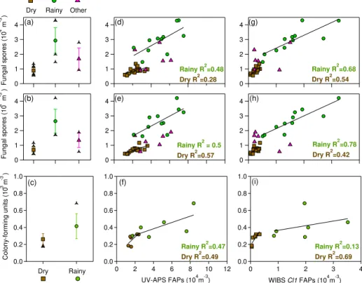
Figure 6.Estimated fungal spore number concentration, calculated using mass of arabitol and mannitol per spore reported by Bauer et al. (2008a). Estimates from arabitol (top row) and mannitol (bottom row). Average fungal spore concentration, calculated using arabitol mass(a), mannitol mass(b), and colony-forming units(c)in each wetness category. Central marker shows mean value of individual filter concentration values, bars represent standard deviation (SD) range of filter values, and individual points show outliers beyond mean±SD. Correlation of fungal spore number calculated from arabitol(d), mannitol(e), and colony-forming units(f)concentrations with estimated fluorescent particle mass from UV-APS. Correlation of fungal spore number calculated from arabitol(g), mannitol(h), and colony-forming unit(i)concentrations with fluorescent particle concentrations from WIBS cluster 1.R2value shown for each fit (right two columns). Linear fit parameters are shown in Table S3.
The first, and most important observation is that the esti-mated fungal spore concentration from each technique is on the same order of magnitude, 104m−3. Looking at individual
correlations reveals a finer layer of detail. These results show that the number concentration of fungal spores estimated by the UV-APS is greater than the number of fungal spores es-timated by the tracers, as evidenced by slope values of ca. 0.2 and 0.35 for Rainy and Dry conditions, respectively (Ta-ble S3, Fig. 6d, e). Again, this suggests that the UV-APS de-tects fungal spores as well as other types of fluorescent par-ticles. The R2values (∼0.5) during Rainy periods indicate that the additional source of particles detected by the UV-APS is likely to have a similar source, such as PBAPs me-chanically ejected from soil and vegetative surfaces with rain splash (Huffman et al., 2013). The magnitude of the over-estimation is higher during Dry periods, which would be ex-pected because Rainy periods exhibited much higher particle number fractions associated with polyol-containing spores.
The Cl1 cluster from WIBS data shows correlations with estimated fungal spores from arabitol and mannitol that have slopes much closer to 1.0 than correlations with UV-APS number (Fig. 6g, h, Table S3). For example, the slope of
the Cl1 correlations with each polyol during Rainy periods is ca. 0.87. This suggests only a 13 % difference between the spore concentration estimates from the two techniques dur-ing Rainy periods. The average number concentration of Cl1 during Rainy periods is 1.6×10⁴(±0.8) spores m−3. In both
cases the slopes with respect to Cl1 are greater than 1.0 dur-ing Dry periods, suggestdur-ing that the cluster method may be missing some fraction of weakly fluorescent particles. Huff-man et al. (2012) similarly suggests that particles that are weakly fluorescent may be below the detection limit of the instrument and Healy et al. (2014) suggested that both UV-APS and WIBS-4 instruments significantly under-count the ubiquitousCladosporiumspores that are most common dur-ing dry weather and often peak in the afternoon when RH is low (De Groot, 1968; Oliveira et al., 2009). Fundamentally, however, the results from the UV-APS, and even more so the numbers reported by the clustering analysis by Crawford et al. (2015), reveal broadly similar trends with the numbers estimated from polyol-to-spore values reported by Bauer et al. (2008a).
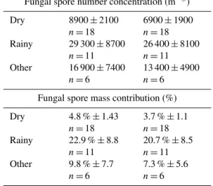
concentra-Table 4.Campaign-average fungal spore concentration and mass contribution estimated from arabitol and mannitol mass measure-ments. Values are mean±standard deviation; n shows number of samples used for averaging. Fungal spore mass assumption of 33 pg spore−1(Bauer et al., 2008b). Total particulate matter mass calculated from UV-APS number concentration (m−3), converted to mass over aerodynamic particle diameter range 0.5–15 µm using 1.5 g cm−3density.
Fungal spore number concentration (m−3)
Dry 8900±2100
n=18
6900±1900 n=18
Rainy 29 300±8700
n=11
26 400±8100 n=11
Other 16 900±7400
n=6
13 400±4900 n=6
Fungal spore mass contribution (%)
Dry 4.8 %±1.43
n=18
3.7 %±1.1 n=18
Rainy 22.9 %±8.8
n=11
20.7 %±8.5 n=11
Other 9.8 %±7.7
n=6
7.3 %±5.6 n=6
tions (Fig. 6c), with an increase of ca. 1.6×during Rainy periods. The trend of a positive slope with respect to the UV-LIF measurements is also similar between the tracer and cul-turing methods. In general, however, theR2value correlat-ing CFU to fungal spore number calculated from the UV-LIF number is lower than between tracers and UV-LIF numbers (Table 3, Fig. S4). This is not unexpected for several rea-sons. First, the short sampling time of the culture samples (20 min) leads to poor-counting statistics and high number concentration variability, whereas each data point from the high-volume air samples represents a period of 4–48 h. Sec-ond, culture samplers, by their nature, only account for cul-turable fungal spores. It has been estimated that as low as 17 % of aerosolized fungal species are culturable, and so it is expected that the CFU concentration observed is signif-icantly less than the total airborne concentration of spores (Bridge and Spooner, 2001; Després et al., 2012). Nonethe-less, the culturing analysis here supports the tracer and UV-LIF analyses and the most important trends are consistent between all analysis methods. The concentration of fungal spores is higher during the Rainy periods, and there is a pos-itive correlation between both tracer and CFU concentration and UV-LIF number.
In a pristine environment, such as the Amazon, supermi-cron particle mass has been found to consist of up to 85 % biological material (Pöschl et al., 2010). Total particulate matter mass was calculated here from the UV-APS number concentrations (m−3)and converted to mass for particles of aerodynamic diameter 0.5–10 µm. In only this case a
den-40
30
20
10
0
Fungal spore mass contribution (%)
40
30
20
10
0
Dry Rainy Other
Arabtiol
Mannitol
(a)
(b)
Figure 7.Estimated fraction of total aerosol mass contributed by fungal spores. Fungal spore mass concentration (µg m−3) calcu-lated separately from mannitol and arabitol concentration and using average mass per spore reported by Bauer et al. (2008b). Total par-ticulate matter mass calculated from UV-APS number concentration (m−3)and converted to mass over aerodynamic particle diameter range 0.5–15 µm using density of 1.5 g cm−3. Central marker shows mean value of individual filter concentration values, bars represent standard deviation (SD) range of filter values, and individual points show outliers beyond mean±SD.
sity of 1.5 g cm−3 was utilized to calculate a first
approxi-mation of total particle mass to which all other mass mea-surements were compared. An average TSP mass density of 1.5 g cm−3was utilized, because organic aerosol is typically
5
4
3
2
1
0
Endotoxins (EU m
-3 )
5
4
3
2
1
0
3 2 1 0
UV-APS FAP (µg m-3
)
5
4
3
2
1
0
12 10 8 6 4 2 0
WIBS ClBact FAP (µg m
-3 ) Dry Rainy Other
(a) (b) (c)
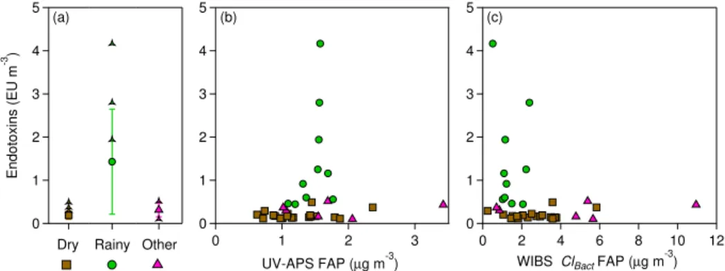
Figure 8.Endotoxin mass concentration as an approximate indicator of gram-negative bacteria concentration.(a)Averaged concentration in each wetness category. Central marker shows mean value of individual filter concentration values, bars represent standard deviation (SD) range of filter values, and individual points show outliers beyond mean±SD.(b)Correlation of endotoxin mass concentration with estimated fluorescent particle mass from UV-APS.(c)Correlation of endotoxin mass concentration with estimated fluorescent particle mass summed from clusters 2, 3, and 4 from Crawford et al. (2015).
3.4 Variations in endotoxin and glucan concentrations Endotoxins measured in the atmosphere are uniquely asso-ciated with gram-negative bacteria (Andreae and Crutzen, 1997). Here, we show correlations between total endotoxin mass and WIBS ClBact, which was assigned by Crawford et
al. (2015) to be bacteria due to the small particle size (< 1 µm) and high correlation with rain. This assignment of particle type to this set of clusters is quite uncertain, however, and should be treated loosely. The correlation between endotoxin mass and UV-APS and the WIBS clusters was very poor, in most casesR2< 0.1 (Table 3, Fig. 8), suggesting no appar-ent relationship. Analysis of bacteria by both UV-LIF tech-niques is hampered by the fact that bacteria can be < 1 µm in size and because both instruments detect particles with decreased efficiency at sizes below 0.8 µm. So weak corre-lations may not have been apparent due to reduced overlap in particle size. Despite the lack of apparent correlation be-tween the techniques, the relatively variable endotoxin con-centrations were elevated during Rainy periods, consistent with Jones and Harrison (2004), who showed that bacteria concentrations were elevated after rainy periods.
Glucans, such as (1→3)-β-D-glucan, are components of the cell walls of pollen, fungal spores, plant detritus, and bac-teria (Chow et al., 2015b; Lee et al., 2006; Stone and Clarke, 1992). In contrast to the observed difference in endotoxin concentration during the different wetness periods, (1→
3)-β-D-glucan showed no correlations with UV-LIF concen-trations (Table 3) and no differentiation during the different wetness periods.
4 Conclusions
Increased concentrations of fluorescent aerosol particles and ice nuclei attributed to having a biological origin were ob-served during and immediately after rain events throughout
the BEACHON-RoMBAS study in 2011 (Huffman et al., 2013; Prenni et al., 2013; Schumacher et al., 2013). Here we expand upon the previous reports by utilizing measure-ments from two commercially available UV-LIF instrumeasure-ments, of several molecular tracers extracted from high-volume fil-ter samples, and from a culture-based sampler in order to compare three very different methods of atmospheric fun-gal spore analysis. This study represents the first reported correlation of UV-LIF and molecular tracer measurements and provides an opportunity to understand how an important class of PBAPs might be influenced by periods of rainy and dry weather. We found clear patterns in the fungal molecular tracers, arabitol and mannitol, associated with Rainy condi-tions that are consistent with previous findings (Bauer et al., 2008a; Elbert et al., 2007; Feofilova, 2001). Fungal polyols increased 3-fold over Dry conditions during Rainy weather samples, with arabitol concentration of 35.2±10.5 ng m−3 and mannitol concentration of 44.9±13.8 ng m−3.
the tracer and UV-LIF approaches to estimating atmospheric fungal spore concentration are fundamentally different, they provide remarkably similar estimates and temporal trends. With further improvements in instrumentation and analysis methods (e.g., advanced clustering algorithms applied to UV-LIF data), the ability to reliably discriminate between PBAP types is improving. As we have shown here, this technol-ogy represents a potential for monitoring approximate fun-gal spore mass and for contributing improved information on fungal spore concentration to global and regional models that to this point has been lacking (Spracklen and Heald, 2014).
5 Data availability
Please contact the author for data used in all plots presented here.
The Supplement related to this article is available online at doi:10.5194/acp-16-15165-2016-supplement.
Acknowledgements. The BEACHON-RoMBAS campaign was
partially supported by an ETBC (Emerging Topics in Biogeochem-ical Cycles) grant to the National Center for Atmospheric Research (NCAR), the University of Colorado, Colorado State University, and Penn State University (NSF ATM-0919189). The authors wish to thank Jose Jimenez, Douglas Day (Univ. Colorado-Boulder); An-thony Prenni, Paul DeMott, Sonia Kreidenweis, and Jessica Prenni (Colorado St. Univ.); Alex Guenther and Jim Smith (NCAR) for BEACHON-RoMBAS project organization and logistical support and the USFS, NCAR, and Richard Oakes for access to the Manitou Experimental Forest Observatory field site. Measurements of temperature, relative humidity, wind speed, and wind direction were provided by Andrew Turnipseed (NCAR) and leaf wetness and disdrometer data were provided by Dave Gochis (NCAR). Marie I. Gosselin thanks the Max Planck Society for financial support. J. Alex Huffman thanks the University of Denver for intra-mural funding for faculty support. The Mainz team acknowledges the Mainz Bioaerosol Laboratory (MBAL) and financial support from the Max Planck Society (MPG), the Max Planck Graduate Center with the Johannes Gutenberg University Mainz (MPGC), the Geocycles Cluster Mainz (LEC Rheinland-Pfalz), and the German Research Foundation (DFG PO1013/5-1 and FR3641/1-2, FOR 1525 INUIT). The Manchester team acknowledges funding from the UK NERC (UK-BEACHON, grant no. NE/H019049/1) for participating in the BEACHON experiment, and development support of the WIBS instruments. Manchester would also like to thank Paul Kaye, the developer of the WIBS instruments and his team at the University of Hertfordshire, for their technical support. The authors thank Cristina Ruzene, Isabell Müller-Germann, Petya Yordanova, Tobias Könemann (Max Planck Inst. For Chem.), and Nicole Savage (Univ. Denver) for technical assistance.
The article processing charges for this open-access publication were covered by the Max Planck Society.
Edited by: J. Surratt
Reviewed by: four anonymous referees
References
Allitt, U.: Airborne fungal spores and the thunderstorm of 24 June 1994, Aerobiologia, 16, 397–406, 2000.
Andreae, M. O. and Crutzen, P. J.: Atmospheric Aerosols: Biogeo-chemical Sources and Role in Atmospheric Chemistry, Science, 276, 1052–1058, doi:10.1126/science.276.5315.1052, 1997. Axelsson, B.-O., Saraf, A., and Larsson, L.: Determination of
ergosterol in organic dust by gas chromatography-mass spec-trometry, J. Chromatogr. B, 666, 77–84, doi:10.1016/0378-4347(94)00553-H, 1995.
Barbaro, E., Kirchgeorg, T., Zangrando, R., Vecchiato, M., Piazza, R., Barbante, C., and Gambaro, A.: Sug-ars in Antarctic aerosol, Atmos. Environ., 118, 135–144, doi:10.1016/j.atmosenv.2015.07.047, 2015.
Bauer, H., Claeys, M., Vermeylen, R., Schueller, E., Weinke, G., Berger, A., and Puxbaum, H.: Arabitol and mannitol as tracers for the quantification of airborne fungal spores, Atmos. Environ., 42, 588–593, doi:10.1016/j.atmosenv.2007.10.013, 2008a. Bauer, H., Schueller, E., Weinke, G., Berger, A., Hitzenberger, R.,
Marr, I. L., and Puxbaum, H.: Significant contributions of fungal spores to the organic carbon and to the aerosol mass balance of the urban atmospheric aerosol, Atmos. Environ., 42, 5542–5549, doi:10.1016/j.atmosenv.2008.03.019, 2008b.
Bigg, E. K., Soubeyrand, S., and Morris, C. E.: Persistent after-effects of heavy rain on concentrations of ice nuclei and rainfall suggest a biological cause, Atmos. Chem. Phys., 15, 2313–2326, doi:10.5194/acp-15-2313-2015, 2015.
Bridge, P. and Spooner, B.: Soil fungi: diversity and detection, Plant Soil, 232, 147–154, 2001.
Buller, A.: Spore deposits – the number of spores, Researches on Fungi, 1, 79–88, 1909.
Burger, H.: Official Publication of American Academy of Allergy and ImmunologyBioaerosols: Prevalence and health effects in the indoor environment, J. Allergy Clin. Immun., 86, 687–701, doi:10.1016/S0091-6749(05)80170-8, 1990.
Burshtein, N., Lang-Yona, N., and Rudich, Y.: Ergosterol, ara-bitol and mannitol as tracers for biogenic aerosols in the eastern Mediterranean, Atmos. Chem. Phys., 11, 829–839, doi:10.5194/acp-11-829-2011, 2011.
Caseiro, A., Marr, I. L., Claeys, M., Kasper-Giebl, A., Puxbaum, H., and Pio, C. A.: Determination of saccharides in atmospheric aerosol using anion-exchange high-performance liquid chro-matography and pulsed-amperometric detection, J. Chromatogr. A, 1171, 37–45, doi:10.1016/j.chroma.2007.09.038, 2007. Cheng, J. Y. W., Hui, E. L. C., and Lau, A. P. S.:
Bioac-tive and total endotoxins in atmospheric aerosols in the Pearl River Delta region, China, Atmos. Environ., 47, 3–11, doi:10.1016/j.atmosenv.2011.11.055, 2012.
Chow, J. C., Lowenthal, D. H., Chen, L.-W. A., Wang, X., and Wat-son, J. G.: Mass reconstruction methods for PM2. 5: a review, Air Quality, Atmosphere & Health, 8, 243–263, 2015a. Chow, J. C., Yang, X., Wang, X., Kohl, S. D., Hurbain, P. R., Chen,