www.geosci-model-dev.net/10/359/2017/ doi:10.5194/gmd-10-359-2017
© Author(s) 2017. CC Attribution 3.0 License.
The Cloud Feedback Model Intercomparison Project (CFMIP)
contribution to CMIP6
Mark J. Webb1, Timothy Andrews1, Alejandro Bodas-Salcedo1, Sandrine Bony2, Christopher S. Bretherton3, Robin Chadwick1, Hélène Chepfer2, Hervé Douville4, Peter Good1, Jennifer E. Kay5, Stephen A. Klein6, Roger Marchand3, Brian Medeiros7, A. Pier Siebesma8, Christopher B. Skinner9, Bjorn Stevens10, George Tselioudis11, Yoko Tsushima1, and Masahiro Watanabe12
1Met Office Hadley Centre, Exeter, UK
2LMD/IPSL, CNRS, Université Pierre and Marie Curie, Paris, France 3University of Washington, Seattle, USA
4Centre National de Recherches Météorologiques, Toulouse, France 5University of Colorado at Boulder, Boulder, USA
6Lawrence Livermore National Laboratory, Livermore, USA 7National Center for Atmospheric Research, Boulder, USA
8Royal Netherlands Meteorological Institute, De Bilt, The Netherlands 9University of Michigan, Ann Arbor, USA
10Max Planck Institute for Meteorology, Hamburg, Germany 11NASA Goddard Institute for Space Studies, New York, USA 12Atmosphere and Ocean Research Institute, Tokyo, Japan Correspondence to:Mark J. Webb ([email protected])
Received: 30 March 2016 – Published in Geosci. Model Dev. Discuss.: 12 May 2016 Revised: 28 October 2016 – Accepted: 31 October 2016 – Published: 25 January 2017
Abstract.The primary objective of CFMIP is to inform fu-ture assessments of cloud feedbacks through improved un-derstanding of cloud–climate feedback mechanisms and bet-ter evaluation of cloud processes and cloud feedbacks in climate models. However, the CFMIP approach is also in-creasingly being used to understand other aspects of climate change, and so a second objective has now been introduced, to improve understanding of circulation, regional-scale pre-cipitation, and nlinear changes. CFMIP is supporting on-going model inter-comparison activities by coordinating a hi-erarchy of targeted experiments for CMIP6, along with a set of cloud-related output diagnostics. CFMIP contributes pri-marily to addressing the CMIP6 questions “How does the Earth system respond to forcing?” and “What are the origins and consequences of systematic model biases?” and supports the activities of the WCRP Grand Challenge on Clouds, Cir-culation and Climate Sensitivity.
A compact set of Tier 1 experiments is proposed for CMIP6 to address this question: (1) what are the physical
mechanisms underlying the range of cloud feedbacks and cloud adjustments predicted by climate models, and which models have the most credible cloud feedbacks? Additional Tier 2 experiments are proposed to address the following questions. (2) Are cloud feedbacks consistent for climate cooling and warming, and if not, why? (3) How do cloud-radiative effects impact the structure, the strength and the variability of the general atmospheric circulation in present and future climates? (4) How do responses in the climate sys-tem due to changes in solar forcing differ from changes due to CO2, and is the response sensitive to the sign of the
forc-ing? (5) To what extent is regional climate change per CO2
doubling state-dependent (non-linear), and why? (6) Are cli-mate feedbacks during the 20th century different to those acting on long-term climate change and climate sensitivity? (7) How do regional climate responses (e.g. in precipitation) and their uncertainties in coupled models arise from the com-bination of different aspects of CO2forcing and sea surface
CFMIP also proposes a number of additional model out-puts in the CMIP DECK, CMIP6 Historical and CMIP6 CFMIP experiments, including COSP simulator outputs and process diagnostics to address the following questions.
1. How well do clouds and other relevant variables simu-lated by models agree with observations?
2. What physical processes and mechanisms are important for a credible simulation of clouds, cloud feedbacks and cloud adjustments in climate models?
3. Which models have the most credible representations of processes relevant to the simulation of clouds?
4. How do clouds and their changes interact with other el-ements of the climate system?
1 Introduction
Inter-model differences in cloud feedbacks continue to be the largest source of uncertainty in predictions of equilibrium cli-mate sensitivity (Boucher et al., 2013). Although the ranges of cloud feedbacks and climate sensitivity from comprehen-sive climate models have not reduced in recent years, con-siderable progress has been made in understanding (a) which types of clouds contribute most to this spread (e.g. Bony and Dufresne, 2005; Webb et al., 2006; Zelinka et al., 2013), (b) the role of cloud adjustments in climate sensitivity (e.g. Gregory and Webb, 2008; Andrews and Forster, 2008; Ka-mae and Watanabe, 2012; Zelinka et al., 2013), (c) the pro-cesses and mechanisms which are (and are not) implicated in cloud feedbacks, both in fine-resolution models (e.g. Rieck et al., 2012; Bretherton et al., 2015) and in comprehensive climate models (e.g. Brient and Bony, 2012; Sherwood et al., 2014; Zhao, 2014; Webb et al., 2015b), (d) the inconstancy of cloud feedbacks and effective climate sensitivity (e.g. Se-nior and Mitchell, 2000; Williams et al., 2008; Andrews et al., 2012; Geoffroy et al., 2013; Armour et al., 2013; Gre-gory and Andrews, 2016) and (e) the extent to which models with stronger or weaker cloud feedbacks or climate sensi-tivities agree with observations (e.g. Fasullo and Trenberth, 2012; Su et al., 2014; Qu et al., 2014; Sherwood et al., 2014; Myers and Norris, 2016). Additionally, our ability to evaluate model clouds using satellite data has benefited from the in-creasing use of satellite simulators. This approach, first intro-duced by Yu et al. (1996) for use with data from the Interna-tional Satellite Cloud Climatology Project (ISCCP), attempts to reproduce what a satellite would observe given the model state. Such approaches enable more quantitative comparisons to the satellite record (e.g. Yu et al., 1996; Klein and Jakob, 1999; Webb et al., 2001; Bodas-Salcedo et al., 2008; Ce-sana and Chepfer, 2013). Much of our improved understand-ing in these areas would have been impossible without the
continuing investment of the scientific community in succes-sive phases of the Coupled Model Intercomparison Project (CMIP) and its co-evolution in more recent years with the Cloud Feedback Model Intercomparison Project (CFMIP).
CFMIP started in 2003 and its first phase (CFMIP-1) or-ganized an intercomparison based on perpetual July SST forced Cess style +2 K experiments and 2×CO2
equilib-rium mixed-layer model experiments containing an ISCCP simulator in parallel with CMIP3 (McAvaney and Le Treut, 2003). CFMIP-1 had a substantial impact on the evaluation of clouds in models and on the identification of low-level cloud feedbacks as the primary cause of inter-model spread in cloud feedback, which featured prominently in the fourth and fifth IPCC assessments (Randall et al., 2007; Boucher et al., 2013).
The subsequent objective of CFMIP-2 was to inform im-proved assessments of climate change cloud feedbacks by providing better tools to support evaluation of clouds simu-lated by climate models and understanding of cloud–climate feedback processes. CFMIP-2 organized further experiments as part of CMIP5 (Bony et al., 2011; Taylor et al., 2012), in-troducing seasonally varying SST perturbation experiments for the first time, as well as fixed SST CO2 forcing
ex-periments to examine cloud adjustments. CFMIP-2 also in-troduced idealized “aquaplanet” experiments into the CMIP family of experiments. These experiments were motivated by extensive research in the framework of the aquaplanet ex-periment (Neale and Hoskins, 2000; Blackburn and Hoskins, 2013) and the particular finding, based on a small subset of models, that the global mean cloud feedback of more realistic model configurations could be reproduced, and more easily investigated, using the much simpler aquaplanet configura-tion (Medeiros et al., 2008). CFMIP-2 proposed the inclusion of the abrupt CO2quadrupling AOGCM (atmosphere–ocean
devel-oped the CFMIP-OBS data portal and the CFMIP Diagnos-tic Codes Catalogue. For more details, and for a full list of CFMIP-related publications, please refer to the CFMIP web-site (http://www.earthsystemcog.org/projects/cfmip).
Studies arising from CFMIP-2 include numerous single-and multi-model evaluation studies which use COSP to make quantitative and fair comparisons with a range of satellite products (e.g. Kay et al., 2012; Franklin et al., 2013; Klein et al., 2013; Lin et al., 2014; Chepfer et al., 2014). COSP has also enabled studies attributing cloud feedbacks and cloud adjustments to different cloud types (e.g. Zelinka et al., 2013, 2014; Tsushima et al., 2016). CFMIP-2 additionally enabled the finding that idealized “aquaplanet” experiments without land, seasonal cycles or Walker circulations are able to repro-duce the essential differences between models’ global cloud feedbacks and cloud adjustments in a substantial ensemble of models (Ringer et al., 2014; Medeiros et al., 2015). Pro-cess outputs from CFMIP have also been used to develop and test physical mechanisms proposed to explain and constrain inter-model spread in cloud feedbacks in the CMIP5 mod-els (e.g. Sherwood et al., 2014; Brient et al., 2015; Webb et al., 2015a; Nuijens et al., 2015a, b; Dal Gesso at al., 2015). CGILS has demonstrated a consensus in the responses of LES models to climate forcings and identified shortcomings in the physical representations of cloud feedbacks in cli-mate models (e.g. Blossey et al., 2013; Zhang et al., 2013; Dal Gesso at al., 2015). The CFMIP experiments have ad-ditionally formed the basis for coordinated experiments to explore the impact of cloud-radiative effects on the circula-tion (Stevens et al., 2012; Fermepin and Bony, 2014; Crueger and Stevens, 2015; Li et al., 2015; Harrop and Hartmann, 2016), the impact of parametrized convection on cloud feed-back (Webb et al., 2015b) and the mechanisms of negative shortwave cloud feedback in mid to high latitudes (Ceppi et al., 2015). Additionally, the CFMIP experiments have, due to their idealized nature, proven useful in a number of studies not directly related to clouds, instead analysing the responses of regional precipitation and circulation patterns to CO2
forc-ing and climate change (e.g. Bony et al., 2013; Chadwick et al., 2014; He and Soden, 2015; Oueslati et al., 2016). Stud-ies using CFMIP-2 outputs from CMIP5 remain ongoing and further results are expected to feed into future assessments of the representation of clouds and cloud feedbacks in climate models.
The primary objective of CFMIP is to inform future as-sessments of cloud feedbacks through improved understand-ing of cloud–climate feedback mechanisms and better evalu-ation of cloud processes and cloud feedbacks in climate mod-els. However, the CFMIP approach is also increasingly be-ing used to understand other aspects of climate change, and so a second objective has been introduced, to improve under-standing of circulation, regional-scale precipitation, and non-linear changes. This involves bringing climate modelling, observational and process modelling communities closer to-gether and providing better tools and community support for
evaluation of clouds and cloud feedbacks simulated by cli-mate models and for understanding of the mechanisms un-derlying them. This is achieved by
– coordinating model inter-comparison activities which include experimental design as well as specification of model output diagnostics to support quantitative evaluation of modelled clouds with observations (e.g. COSP) and in situ measurements (e.g. cfSites) as well as process-based investigation of cloud maintenance and feedback mechanisms (e.g. cfSites, temperature and hu-midity tendency terms);
– developing and improving support infrastructure, in-cluding COSP, CFMIP-OBS and the CFMIP Diagnostic Codes Catalogue; and
– fostering collaboration with the observational and cloud process modelling communities via annual CFMIP meetings and internationally funded projects.
CFMIP is now entering its third phase, CFMIP-3, which will run in parallel with the current phase of the Coupled Model Intercomparison Project (CMIP6, Eyring et al., 2016). This paper documents the CFMIP-3/CMIP6 experiments and di-agnostic outputs which constitute the CFMIP-3 contribution to CMIP6. It is anticipated that CFMIP-3 will be broader than what is described here, for instance including studies with process models and informal CFMIP-3 experiments which are organized independently of CMIP6. Please refer to the CFMIP website for announcements of these other initiatives and CFMIP annual meetings.
CFMIP-3 touches, to differing degrees, on each of the three questions around which CMIP6 is organized. With its focus on cloud feedback, CFMIP-3 is central to CMIP6’s at-tempt to answer the question “How does the Earth system respond to forcing?”, but as illustrated in the remainder of this document, CFMIP-3 also offers the opportunity to con-tribute to the other two guiding questions of CMIP6. Through its strong model evaluation component, it stands to help to answer the question “What are the origins and consequences of systematic model biases?”. CFMIP-3 will also help an-swer the question “How can we assess future climate changes given climate variability, climate predictability, and uncer-tainties in scenarios?”. For example, theamip-piForcing ex-periment proposed below will support studies relating cloud variability and feedbacks on observable timescales to long-term cloud feedbacks (Andrews, 2014; Gregory and An-drews, 2016).
piControl 1pctCO2 Pre-industrial
clouds and precipitation
Historical / present day clouds and precipitation
CO2forcing, cloud
and precipitation adjustments
Climate feedbacks and precipitation responses
abrupt-4xCO2 CMIP6 historical
amip-4xCO2
amip amip-p4K
aqua-control aqua-4xCO2
amip-future4K
abrupt-0p5xCO2 amip-piForcing
abrupt-solp4p aqua-p4K
amip-lwoff amip-p4K-lwoff
aqua-control-lwoff
piSST-4xCO2-rad
piSST a4SST piSST-pxK
amip-m4K
a4SSTice-4xCO2 a4SSTice
amip-a4SST-4xCO2 piSST-4xCO2
abrupt-solm4p
DECK/CMIP6
aqua-p4K-lwoff
CFMIP Tier 1
CFMIP Tier 2
abrupt-2xCO2
C
lo
u
d
s Circ
u
la
tio
n
a
n
d
pr
e
c
ip
ita
tio
n
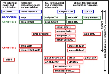
Figure 1.Summary of CFMIP-3/CMIP6 experiments and DECK+ CMIP6 Historical experiments.
2 CFMIP-3 experiments
The CFMIP-3/CMIP6 experiments are summarized in Fig. 1 and Tables 1 and 2, and are described in detail below. Most of the CFMIP-3/CMIP6 experiments are based on CO2
concentration forced amip, piControl and abrupt-4xCO2 CMIP DECK (Diagnostic, Evaluation and Characterization of Klima) experiments (Eyring et al., 2016). Unless oth-erwise specified below, the CFMIP-3/CMIP6 experiments should be configured consistently with the DECK experi-ments on which they are based, using consistent model for-mulation, and forcings and boundary conditions as speci-fied by Eyring et al. (2016). Following the CMIP6 design protocol, groups of experiments are motivated by science questions and are separated into Tiers 1 and 2 (Eyring et al., 2016). It is a requirement for participation by modelling groups in the CFMIP-3/CMIP6 model intercomparison that all Tier 1 experiments be performed and published through the ESGF, so as to support CFMIP’s Tier 1 science question. Tier 2 experiments are optional, and are associated with ad-ditional science questions. Any subset of Tier 2 experiments may be performed. All model output archived by CFMIP-3/CMIP6 is expected to be made available under the same terms as CMIP output. Most modelling groups currently re-lease their CMIP data for unrestricted use. Our analysis plans for the CFMIP-3/CMIP6 experiments are summarized in Ap-pendix A.
2.1 CFMIP-3/CMIP6 Tier 1 experiments Lead coordinator: Mark Webb
Science question: what are the physical mechanisms underlying the range of cloud feedbacks and cloud adjust-ments predicted by climate models, and which of the cloud
responses are the most credible?
Equilibrium climate sensitivity (ECS) can be estimated us-ing an idealized AOGCM experiment such as the abrupt-4xCO2experiment in the CMIP6 DECK, at the same time statistically separating the global mean contributions from climate feedbacks and adjusted radiative forcing due to CO2
(Gregory et al., 2004; Andrews et al., 2012). However, un-derstanding the physical processes underlying cloud feed-backs and adjustments requires diagnosis in SST forced ex-periments with atmosphere-only general circulation models (AGCMs), which can resolve cloud feedbacks and adjust-ments independently of each other and with minimal sta-tistical noise at regional scales, while faithfully reproducing the inter-model differences in global values from the fully coupled models (Ringer et al., 2014). (The ability of these AGCM experiments to reproduce the inter-model differences in global cloud feedbacks and adjustments from coupled models indicates that they do not strongly depend on differ-ent ocean model formulations or SST biases.) The CFMIP-2/CMIP5amip4xCO2experiments, which quadrupled CO2
while leaving SSTs at present-day values (Bony et al., 2011), allowed the land–tropospheric adjustment process and the cloud adjustment to CO2to be examined in this way for the
first time in the multi-model context (Kamae and Watanabe, 2012; Ringer at al., 2014; Kamae et al., 2015) in conjunction with the CMIP5sstClim/sstClim4xCO2experiments which were based on climatological pre-industrial SSTs (Andrews et al., 2012; Zelinka et al., 2013; Vial et al., 2013). These experiments have additionally formed the basis for more in-depth studies with individual models (e.g. Wyant et al., 2012; Kamae and Watanabe, 2013; Bretherton et al., 2014; Ogura et al., 2014). The CFMIP-2/CMIP5amip4KandamipFuture SST perturbed atmosphere-only experiments (Bony et al., 2011) have been used to examine cloud feedbacks in greater detail (e.g. Brient and Bony, 2012; Bretherton et al., 2014; Lacagnina et al., 2014; Bellomo and Clement, 2015; Webb et al., 2015b), often in conjunction with simulator outputs (e.g. Gordon and Klein, 2014; Chepfer et al., 2014; Tsushima et al., 2016; Ceppi et al., 2016) and CFMIP process diagnos-tics (e.g. Webb and Lock, 2013; Sherwood et al., 2014; Bri-ent et al., 2015; Webb et al., 2015a; Dal Gesso at al., 2015). Similarly, these experiments have been used to investigate re-gional responses of various quantities to direct radiative forc-ing due to increasforc-ing CO2concentrations and/or increases in
SST, including precipitation (e.g. Ma and Xie, 2013; Huang et al., 2013; Widlansky et al., 2013; Kent et al., 2015; Long et al., 2016), circulation (e.g. He et al., 2014; Zhou et al., 2014; Kamae et al., 2014; Bellomo and Clement, 2015; Shaw and Voigt, 2015) and stability (e.g. Qu et al., 2015).
ad-Table 1.Summary of CFMIP-3/CMIP6 Tier 1 experiments.
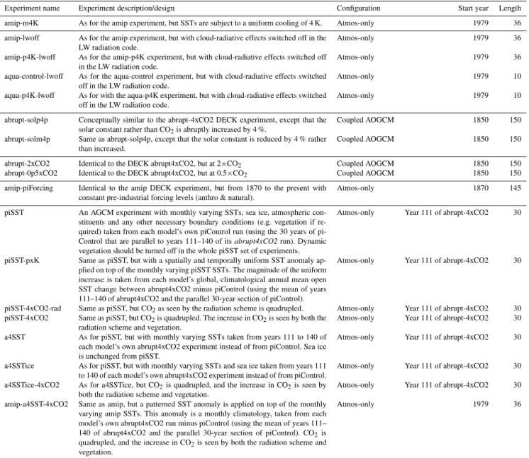
Experiment name Experiment description/design Configuration Start year Length
amip This is a single ensemble member of the AMIP DECK experiment which
con-tains additional outputs which are required for model evaluation using COSP, and as control values for model outputs in the p4K, 4xCO2, amip-future4K and amip-m4K experiments.
Atmos-only 1979 36
amip-p4K As for the CFMIP-2/CMIP5 amip4K experiment. AMIP experiment where
SSTs are subject to a uniform warming of 4 K.
Atmos-only 1979 36
amip-4xCO2 As for the CFMIP-2/CMIP5 amip4xCO2 experiment. AMIP experiment where
SSTs are held at control values and the CO2seen by the radiation scheme is quadrupled.
Atmos-only 1979 36
amip-future4K As for the CFMIP-2/CMIP5 amipFuture experiment. AMIP experiment where SSTs are subject to a composite SST warming pattern derived from coupled models, scaled to an ice-free ocean mean of 4 K.
Atmos-only 1979 36
aqua-control Extended version of the CFMIP-2/CMIP5 aquaControl experiment. Aquaplanet (no land) experiment with no seasonal cycle forced with specified zonally sym-metric SSTs.
Atmos-only 1979 10
aqua-p4K Extended version of the CFMIP-2/CMIP5 aqua4K experiment. Aquaplanet
ex-periment where SSTs are subject to a uniform warming of 4 K.
Atmos-only 1979 10
aqua-4xCO2 Extended version of the CFMIP-2/CMIP5 aqua4xCO2 experiment. Aquaplanet
experiment where SSTs are held at control values and the CO2seen by the radiation scheme is quadrupled.
Atmos-only 1979 10
justments and feedbacks from realistic experiments surpris-ingly effectively (Medeiros et al., 2008, 2015; Ringer et al., 2014), as well as many aspects of the zonal mean circulation response (Medeiros et al., 2015). This indicates that those features of the climate system excluded from these exper-iments (i.e. the ocean, land, seasonal cycle, monsoon and Walker circulations) are not central to understanding inter-model differences in global mean cloud feedbacks and ad-justments, and demonstrates the value of aquaplanet experi-ments for investigating the origin of such differences, as well as differences in zonally averaged precipitation and circula-tion and their responses to climate change (e.g. Stevens et al., 2012; Bony et al., 2013; Oueslati and Bellon, 2013; Fer-mepin and Bony, 2014; Voigt and Shaw, 2015). The aqua-planet experiments have the benefit not only of being less computationally expensive than alternative experiments (re-quiring only 5–10 years to get a robust signal); they are also much more straightforward to analyse, as their behaviour can mostly be characterized by examining zonal means, avoiding the analysis overhead of compositing which is generally re-quired in realistic model configurations to isolate the various cloud regimes. Aquaplanet simulations (and other idealized experiments) are particularly effective at highlighting model differences, for instance in the placement of the tropical rain bands, or in the representation of cloud changes with warm-ing, as it is not possible to tune them to observations in the same way as for more realistic configurations (e.g. Stevens and Bony, 2013).
The CFMIP-2/CMIP5 experiments and diagnostic out-puts have thus enabled considerable progress on a num-ber of questions. However, participation by a larger fraction of modelling groups is desired in CFMIP-3/CMIP6 to
en-able a more comprehensive assessment of the uncertainties across the full multi-model ensemble. Our proposal is there-fore to retain the CFMIP-2/CMIP5 experiments (known in CMIP5 asamip4K, amip4xCO2, amipFuture, aquaControl, aqua4xCO2 and aqua4K) in Tier 1 for CFMIP-3/CMIP6. These are summarized in Table 1 (the names have been changed slightly compared to the CMIP5 equivalents to fit in with the wider naming convention of CMIP6). The set-up for each of these experiments is described below. (For output requirements from these and other experiments, please refer to Sect. 3.)
– amip: this is a single ensemble member of the CMIP DECKamipexperiment which contains additional out-puts which are required both for model evaluation using COSP and for interpretation of feedbacks and adjust-ments in conjunction with theamip-p4K, amip-4xCO2, amip-future4Kandamip-m4Kexperiments.
– amip-p4K(formerly amip4K): the same as the AMIP DECK experiment, except that SSTs are subject to a uniform warming of 4 K. This warming should be ap-plied to the ice-free ocean surface only. Sea ice and SSTs in grid boxes containing sea ice remain the same as in the AMIP DECK experiment.
Table 2.Summary of CFMIP-3/CMIP6 Tier 2 experiments.
Experiment name Experiment description/design Configuration Start year Length
amip-m4K As for the amip experiment, but SSTs are subject to a uniform cooling of 4 K. Atmos-only 1979 36
amip-lwoff As for the amip experiment, but with cloud-radiative effects switched off in the LW radiation code.
Atmos-only 1979 36
amip-p4K-lwoff As for the amip-p4K experiment, but with cloud-radiative effects switched off in the LW radiation code.
Atmos-only 1979 36
aqua-control-lwoff As for the aqua-control experiment, but with cloud-radiative effects switched off in the LW radiation code.
Atmos-only 1979 10
aqua-p4K-lwoff As for with the aqua-p4K experiment, but with cloud-radiative effects switched off in the LW radiation code.
Atmos-only 1979 10
abrupt-solp4p Conceptually similar to the abrupt-4xCO2 DECK experiment, except that the solar constant rather than CO2is abruptly increased by 4 %.
Coupled AOGCM 1850 150
abrupt-solm4p Same as abrupt-solp4p, except that the solar constant is reduced by 4 % rather than increased.
Coupled AOGCM 1850 150
abrupt-2xCO2 Identical to the DECK abrupt4xCO2, but at 2×CO2 Coupled AOGCM 1850 150
abrupt-0p5xCO2 Identical to the DECK abrupt4xCO2, but at 0.5×CO2 Coupled AOGCM 1850 150
amip-piForcing Identical to the amip DECK experiment, but from 1870 to the present with constant pre-industrial forcing levels (anthro & natural).
Atmos-only 1870 145
piSST An AGCM experiment with monthly varying SSTs, sea ice, atmospheric con-stituents and any other necessary boundary conditions (e.g. vegetation if re-quired) taken from each model’s own piControl run (using the 30 years of pi-Control that are parallel to years 111–140 of itsabrupt4xCO2run). Dynamic vegetation should be turned off in the whole piSST set of experiments.
Atmos-only Year 111 of abrupt-4xCO2 30
piSST-pxK Same as piSST, but with a spatially and temporally uniform SST anomaly ap-plied on top of the monthly varying piSST SSTs. The magnitude of the uniform increase is taken from each model’s global, climatological annual mean open SST change between abrupt4xCO2 minus piControl (using the mean of years 111–140 of abrupt4xCO2 and the parallel 30-year section of piControl).
Atmos-only Year 111 of abrupt-4xCO2 30
piSST-4xCO2-rad Same as piSST, but CO2as seen by the radiation scheme is quadrupled. Atmos-only Year 111 of abrupt-4xCO2 30
piSST-4xCO2 Same as piSST, but CO2is quadrupled. The increase in CO2is seen by both the
radiation scheme and vegetation.
Atmos-only Year 111 of abrupt-4xCO2 30
a4SST As for piSST, but with monthly varying SSTs taken from years 111 to 140 of each model’s own abrupt4xCO2 experiment instead of from piControl. Sea ice is unchanged from piSST.
Atmos-only Year 111 of abrupt-4xCO2 30
a4SSTice As for piSST, but with monthly varying SSTs and sea ice taken from years 111 to 140 of each model’s own abrupt4xCO2 experiment instead of from piControl.
Atmos-only Year 111 of abrupt-4xCO2 30
a4SSTice-4xCO2 As for a4SSTice, but CO2is quadrupled, and the increase in CO2is seen by
both the radiation scheme and vegetation.
Atmos-only Year 111 of abrupt-4xCO2 30
amip-a4SST-4xCO2 Same as amip, but a patterned SST anomaly is applied on top of the monthly varying amip SSTs. This anomaly is a monthly climatology, taken from each model’s own abrupt4xCO2 run minus piControl (using the mean of years 111– 140 of abrupt4xCO2 and the parallel 30-year section of piControl). CO2is
quadrupled, and the increase in CO2is seen by both the radiation scheme and
vegetation.
Atmos-only 1979 36
ice should remain the same as in the AMIP DECK ex-periment. The warming pattern should be scaled to en-sure that the global mean SST increase averaged over the ice-free oceans is 4 K. Care should be taken to en-sure that SSTs are increased in any inland bodies of wa-ter and near coastal edges, for example by linearly inwa-ter- inter-polating the provided warming pattern dataset to fill in missing data before re-gridding to the target resolution. – amip-4xCO2 (formerly amip4xCO2): the same as the amip experiment within DECK, except that the CO2
concentration seen by the radiation scheme is quadru-pled. The CO2 seen by the vegetation should be the
same as in the AMIP DECK experiment. This ex-periment gives an indication of the adjusted radia-tive forcing due to CO2quadrupling, including
strato-spheric, land surface, tropospheric and cloud adjust-ments. (Given the names of other CMIP6 experiments, this experiment might have been better named amip-4xCO2-rad, but this inconsistency was only noticed af-ter the experiment names were finalized and propagated to the ESGF.)
The configurations of theaqua-control, aqua-p4Kand aqua-4xCO2experiments are unchanged compared to their equiv-alents in CFMIP-2/CMIP5, except that the simulation length has been extended to 10 years to improve the signal-to-noise ratio. Further details of their experimental set-up are included in Appendix B.
Sen-sitivity (Bony et al., 2015). These will include for exam-ple sensitivity experiments to assess the impacts of different physical processes on cloud feedbacks and regional circula-tion/precipitation responses and also to test specifically pro-posed cloud feedback mechanisms (e.g. Webb et al., 2015b; Ceppi et al., 2015). Additional experiments further idealiz-ing the aquaplanet framework to a non-rotatidealiz-ing rotationally symmetric case are also under development (e.g. Popke et al., 2013). These will be proposed as additional Tier 2 exper-iments at a future time or coordinated informally outside of CMIP6.
2.2 amip minus 4 K experiment (Tier 2) Lead coordinators: Mark Webb and Bjorn Stevens
Science question: are cloud feedbacks consistent for climate cooling and warming, and, if not, why?
There is some evidence to suggest that cloud feedbacks might operate differently in response to cooling rather than warming. For example, Yoshimori et al. (2009) found a posi-tive shortwave cloud feedback in a CO2doubling experiment
with a particular GCM, but noted a tendency for it to become weaker or even negative in cooling experiments designed to replicate the climate of the Last Glacial Maximum. They sug-gested that this might be related to different displacements of mixed-phase clouds in the two scenarios. For small enough changes where linearity is a good approximation, one would expect the cloud response to cooling and warming to be the same, differing only in sign, resulting in an identical cloud feedback expressed per degree of global temperature change, but for larger perturbations this symmetry of response may no longer hold. A warming or cooling of the atmosphere of equal magnitude while maintaining relative humidity will for example generate different changes in absolute humidity and its horizontal and vertical gradients, which have been linked to cloud feedbacks (Brient and Bony, 2013; Sherwood et al., 2014), the atmospheric lapse rate and circulation which in-fluences clouds and depends in part on the absolute humidity (Held and Soden, 2006; Qu et al., 2015) and additionally on extratropical cloud optical depth feedbacks which may be re-lated to adiabatic cloud liquid water contents (Gordon and Klein, 2014) or phase changes that depend upon whether a given volume crosses the 0◦isotherm in the climate change
(Ceppi et al., 2015).
The configuration of theamip-m4Kexperiment will be the same as the amip-p4Kexperiment, except that the sea sur-face temperatures are uniformly reduced by 4 K rather than increased. This cooling should be applied to sea-ice-free grid boxes only. Sea ice and SSTs in grid boxes containing sea ice should remain the same as in the AMIP DECK experi-ment. In models which employ a fixed lower threshold near freezing for the SST used in the calculation of the surface fluxes, this should ideally also be reduced by 4 K. This
ex-periment will contain CFMIP COSP and process outputs so as to support the investigation of inconsistent responses of clouds to a cooling vs. a warming climate in a controlled way through comparison with the amip-p4K experiment. This experiment also complements the abrupt 0.5×CO2 and the
−4 % solar experiments in that one can identify asymme-tries in the warming/cooling response with and without in-teractions with the ocean. As such we hope that these exper-iments will provide useful synergies with the Palaeoclimate Model Intercomparision Project (PMIP) CMIP6 experiments (Kageyama et al., 2016), for example in interpreting differing cloud feedbacks between future CO2forced experiments and
those representing the Last Glacial Maximum, as highlighted by Yoshimori et al. (2009).
2.3 Atmosphere-only experiments without longwave cloud-radiative effects (Tier 2)
Lead coordinators: Sandrine Bony and Bjorn Stevens Science question: how do cloud-radiative effects impact the structure, the strength and the variability of the general atmospheric circulation in present and future climates?
It is increasingly recognized that clouds, and atmospheric cloud-radiative effects in particular, play a critical role in the general circulation of the atmosphere and its response to global warming or other perturbations: they have been found to modulate the structure, the position and shifts of the ITCZ (e.g. Slingo and Slingo, 1988; Randall et al., 1989; Sherwood et al., 1994; Bergman and Hendon, 2000; Hwang and Frier-son, 2013; Fermepin and Bony 2014; Voigt et al., 2014; Loeb et al., 2015), the organization of convection in tropical waves, Madden–Julian oscillations and other forms of convective aggregation (e.g. Lee et al., 2001; Lin et al., 2004; Bony and Emanuel, 2005; Zurovac-Jevtic et al., 2006; Crueger and Stevens, 2015; Muller and Bony, 2015), the extra-tropical cir-culation and the position of eddy-driven jets (e.g. Ceppi et al., 2012, 2014; Grise and Polvani, 2014; Li et al., 2015; Voigt and Shaw, 2015), and modes of inter-annual to decadal cli-mate variability (e.g. Bellomo et al., 2015; Rädel et al., 2016; Yuan et al., 2016). A better assessment of this role would greatly help to interpret model biases (how much do biases in cloud-radiative properties contribute to biases in the struc-ture of the ITCZ, in the position and strength of the storm tracks, in the lack of intra-seasonal variability, etc.) and to inter-model differences in simulations of the current climate and in climate change projections (especially changes in re-gional precipitation and extreme events). More generally, a better understanding of how clouds couple to the circulation is expected to improve our ability to answer the four science questions raised by the WCRP Grand Challenge on Clouds, Circulation and Climate Sensitivity (Bony et al., 2015).
(COOKIE) project proposed by European consortium EU-CLIPSE and CFMIP (Stevens et al., 2012). The COOKIE ex-periments, which have been run by four to eight climate mod-els (depending on the experiment), switched off the cloud-radiative effects (clouds seen by the radiation code – and the radiation code only – were artificially made transparent) in an atmospheric model forced by prescribed SSTs. By do-ing so, the atmospheric circulation could feel the lack of cloud-radiative heating within the atmosphere, but the land surface could also feel the lack of cloud shading, which led to changes in land surface temperatures and land–sea con-trasts. The change in circulation between On and Off ex-periments resulted from both effects, obscuring to some de-gree the mechanisms through which the atmospheric cloud-radiative effects interact with the circulation for given surface boundary conditions. As the longwave cloud-radiative effects are felt mostly within the troposphere (representing most of the net atmospheric cloud-radiative heating), while the short-wave effects are felt mostly at the surface (e.g. L’Ecuyer and McGarragh, 2010; Haynes et al., 2013), we could better iso-late the role of tropospheric cloud-radiative effects on the cir-culation by running atmosphere-only experiments in which clouds are made transparent to radiation only in the long-wave. In this configuration, the models will have a short-wave cloud feedback but no longshort-wave cloud feedback. We note that the presence of clouds does affect the shortwave radiative heating of the atmosphere, although this is a much smaller effect than its longwave equivalent (e.g. Pendergrass and Hartmann, 2014).
Therefore we propose in Tier 2 a set of simple experiments similar to the amip,amip-p4K,aqua-control andaqua-p4K experiments within Tier 1, but in which cloud-radiative ef-fects are switched off in the longwave part of the radiation code while retaining those in the shortwave part (Fermepin and Bony, 2014). Care should also be taken to remove the ef-fects of cloud on any longwave cooling used in other model schemes (e.g. turbulent mixing) if these are calculated inde-pendently of the radiation scheme. These experiments will be referred to asamip-lwoff, amip-p4K-lwoff, aqua-control-lwoffandaqua-p4K-lwoff. The analysis of idealized (aqua-planet) experiments will allow us to assess the robustness of the impacts found in more realistic (AMIP) configurations. It will also facilitate the interpretation of the results using simple dynamical models or theories, in collaboration with large-scale dynamicists (e.g. DynVar). The comparison of the inter-model spread of simulations between the standard and “lwoff” experiments for present-day and warmer cli-mates will help to identify which aspects of the inter-model spread depend on the representation of cloud-radiative ef-fects, and which aspects do not, thus better highlighting other sources of spread. An alternative method (proposed by Aiko Voigt) was also considered, in which clear-sky heating rates would be applied in the atmosphere while retaining the all-sky fluxes at the surface. Although this approach would po-tentially isolate the effects of cloud heating in the atmosphere
more cleanly than the lwoff experiments proposed here, it is yet to be demonstrated in a pilot study, and is considered more technically difficult to implement than the lwoff exper-iments, which are very similar to those piloted by Fermepin and Bony (2014).
2.4 Abrupt±4 % solar forced AOGCM experiments (Tier 2)
Lead coordinators: Chris Bretherton, Roger Marchand, and Bjorn Stevens
Science question: how do responses in the climate system due to changes in solar forcing differ from changes due to CO2, and is the response sensitive to the sign of the solar
forcing?
While rapid adjustments in clouds and precipitation can easily be separated from conventional feedbacks in SST forced experiments, such a separation in coupled models is complicated by various issues, including the response of the ocean on decadal timescales. A number of studies have ex-amined cloud feedbacks in coupled models subject to a so-lar forcing, which is generally associated with much smaller global cloud and precipitation adjustment, due to a smaller atmospheric absorption for a given top of atmosphere forc-ing (e.g. Lambert and Faull, 2007; Andrews et al., 2010), but the regional cloud and precipitation changes have yet to be rigorously investigated across models. Solar forcing also dif-fers from greenhouse forcing through its different fingerprint on the vertical structure of warming (Santer et al., 2013) and small changes in the radiative heating near the tropopause may project measurably on tropospheric climate (e.g. Butler et al., 2010), for instance by influencing the baroclinicity in the upper troposphere and thus the storm tracks (Bony et al., 2015).
A +4 % solar experiment abrupt-solp4p is proposed which is analogous to the abrupt-4xCO2 experiment, but rather than changing CO2it would abruptly increase the
so-lar constant by 4 % and keep it fixed for 150 years, result-ing in a global mean radiative forcresult-ing of a similar magnitude to that due to CO2 quadrupling. When changing the solar
constant, the shape of the spectral solar irradiance distribu-tion should remain consistent with that in the piControl ex-periment. This experiment complements the DECK abrupt-4xCO2experiment, tests the forcing feedback framework for analysing climate change, and would support our understand-ing of regional responses of the coupled system with and without CO2adjustments. The complementary−4 % abrupt
2.5 nonLinMIP abrupt 2×CO2and abrupt 0.5×CO2 experiments (Tier 2)
Lead coordinator: Peter Good
Science question: to what extent is regional-scale climate change per CO2doubling state-dependent (non-linear); what
are the associated mechanisms; and how does this affect our understanding of climate model uncertainty?
Recent studies with individual, or a small number of climate models, have found substantial non-linearities in regional-scale precipitation change (Good et al., 2012; Chad-wick and Good, 2013) associated with robust physical mechanisms (Chadwick and Good, 2013). Significant non-linearity has also been found in global- and regional-scale warming (e.g. Colman and McAvaney, 2009; Jonko et al., 2013; Good et al., 2015; Meraner et al., 2013) and ocean heat uptake (Bouttes et al., 2015).
To address this science question, we propose two new experiments for Tier 2, abrupt2xCO2andabrupt0p5xCO2. These are the same as the DECKabrupt4xCO2experiment except that CO2concentrations are doubled and halved,
re-spectively, relative to the pre-industrial control. These exper-iments are based on a proven analysis approach, including traceability of these experiments to transient-forcing simu-lations (Good et al., 2016), to explore global- and regional-scale non-linear responses, highlighting different behaviour under business-as-usual scenarios, mitigation scenarios and palaeoclimate simulations. Additionally, comparisons of the abrupt-2xCO2 andabrupt-4xCO2experiments will help to establish the extent to which the latter accurately estimates the equilibrium climate sensitivity to CO2 doubling (e.g.
Gregory et al., 2004; Block and Mauritsen, 2013). Additional experiments (Good et al., 2016) may be proposed for Tier 2 in the future, or coordinated informally by CFMIP-3 out-side of CMIP6. These include 100-year extensions to abrupt-4xCO2andabrupt-2xCO2, a 1 % ramp-down from the end of the1pctCO2experiment, and an abrupt step-down to 1×CO2
from year 100 of the abrupt-4xCO2. These would be used to explore longer-timescale responses, quantify non-linear mechanisms more precisely and understand the reversibility of climate change.
2.6 Feedbacks inamipexperiments (Tier 2) Lead coordinator: Timothy Andrews
Science question: are climate feedbacks during the 20th century different to those acting on long-term climate change?
Recent studies have shown significant time variation in cli-mate feedbacks in response to CO2 quadrupling (e.g.
An-drews et al., 2012, 2015; Geoffroy et al., 2013; Armour et
al., 2013). This raises the possibility that feedbacks during the 20th century may be different to those acting on long-term change and hence have the potential to alleviate the ap-parent discrepancy between estimates of climate sensitivity from comprehensive climate models and from simple cli-mate models fitted to observed warming trends (Collins et al., 2013). For example, Gregory and Andrews (2016) found that two models forced with observed monthly 20th century SST and sea-ice variations simulated effective climate sensi-tivities of about 2 K, whereas these same models forced with patterns of long-term SST change simulated effective climate sensitivities of over 3 and 4 K.
The previous CFMIP-2/CMIP5 design was unable to di-agnose the time variation of feedbacks of explicit relevance to the historical period, because this requires the removal of the time-varying forcing. To address this we propose an addi-tional experiment calledamip-piForcing(amippre-industrial forcing) following the design of Andrews (2014) and Gre-gory and Andrews (2016). This experiment is the same as the AMIP DECK experiment (i.e. using observed monthly updating SSTs and sea ice), but run for the period 1870– present and with constant pre-industrial forcings (i.e. all an-thropogenic and natural forcing boundary conditions iden-tical to the piControl experiment). Since the forcing con-stituents do not change in this experiment, it readily allows a simple diagnosis of the simulated atmospheric feedbacks to observed SST and sea-ice changes, which can then be com-pared to feedbacks representative of long-term change and climate sensitivity (e.g. fromabrupt-4xCO2 or amip-p4K). The experiment has the additional benefit, by differencing with the standardamiprun that includes time-varying forc-ing agents, of providforc-ing detailed information on the tran-sient effective radiative forcing and adjustments in models during theamipperiod (Andrews, 2014). This can then be compared to the forcings diagnosed in the Radiative Forc-ing Model Intercomparison Project (RFMIP, Pincus et al., 2016, who use a pre-industrial climate baseline) to test for any dependence of forcing and adjustments on the climate state. Time-varying feedbacks in theamipexperiment could alternatively be diagnosed by subtracting a time-varying ra-diative forcing diagnosed from RFMIP experiments. How-ever, the amip-piForcingapproach has the benefit of diag-nosing the time-varying feedbacks over the full 1870–present period rather than the last 36 years, and does so with refer-ence to a single experiment, which reduces noise compared to that which would be present with a double difference of the amipexperiment and two RFMIP experiments. Also, the in-clusion of CFMIP process diagnostics in theamip-piForcing experiment will enable a deeper understanding of the factors underlying forcing and feedback differences in the present and future climate.
et al. (2015) investigated such effects using two atmosphere-only GCMs forced with SSTs and sea ice from their own abrupt-4xCO2experiments, and attributed the time variation in the feedbacks to changes in the pattern of surface warm-ing. Pilot studies are ongoing to develop similar experiments based on a composite SST pattern response more represen-tative of the CMIP5 ensemble mean. We plan to organize an informal pilot intercomparison based on this within CFMIP-3 and may subsequently propose these experiments as an ex-tension to the CFMIP-3/CMIP6 experiment set.
2.7 Time slice experiments for understanding regional climate responses to CO2(Tier 2)
Lead coordinators: Robin Chadwick, Hervé Douville and Christopher Skinner
Science questions:
– How do regional climate responses (e.g. of precipita-tion) in a coupled model arise from the combination of responses to different aspects of CO2 forcing and sea
surface warming (uniform SST warming, patterned SST warming, sea-ice change, direct CO2effect, plant
phys-iological effect)?
– Which aspects of forcing/warming are most important for causing inter-model uncertainty in regional climate projections?
– Can inter-model differences in regional projections be related to underlying structural or resolution differences between models through improved process understand-ing, and could this help us to constrain the range of re-gional projections?
– What impact do coupled model SST biases have on re-gional climate projections?
The CFMIP-2/CMIP5 set of idealized amipexperiments (e.g.amip4K,amipFuture) have allowed the contribution of different aspects of SST warming and increased CO2
con-centrations to the projections of fully coupled GCMs to be examined (e.g. Bony et al., 2013; Chadwick et al., 2014; He and Soden, 2015). However, theamipexperiments were not designed to replicate coupled GCM responses on a re-gional scale, and large discrepancies exist between the two in many regions, particularly when individual models are exam-ined instead of the ensemble mean (Chadwick, 2016). This is largely due to the choice of present-day and future SST boundary conditions used in theamipexperiments, as well as missing processes such as the plant physiological response to CO2, rather than the lack of air–sea coupling (Skinner et al.,
2012).
We propose a new set of seven 30-year atmosphere-only time slice experiments, and one 36-year amip-style experi-ment, to decompose the regional responses of each model’s
abrupt-4xCO2run into separate responses to each aspect of forcing and warming (uniform SST warming, pattern SST change, sea-ice change, increased CO2, plant physiological
effect). These are forced with monthly and annually varying monthly mean SSTs and sea ice, which reproduce regional precipitation patterns more accurately than is possible using climatological SST forcing (Skinner et al., 2012). As well as allowing regional responses in each individual model to be better understood, this set of experiments should prove especially useful for understanding the causes of model un-certainty in regional climate change.
The experiments are
1. piSST– an AGCM experiment with monthly and an-nually varying SSTs, sea ice, atmospheric constituents and any other necessary boundary conditions (e.g. veg-etation if required) taken from a section of each model’s ownpiControlrun, using the 30 years ofpiControlthat are parallel to years 111–140 of itsabrupt-4xCO2run. Note that dynamic vegetation (if included in the model) should not be turned on in any of thepiSSTset of exper-iments;
2. piSST-pxK– same aspiSST, but with a global spatially and temporally uniform SST anomaly applied on top of the monthly – and annually – varyingpiSSTSSTs. The magnitude of the uniform increase is taken from each model’s global, climatological annual mean open SST change betweenabrupt-4xCO2andpiControl(using the mean of years 111–140 ofabrupt-4xCO2and the paral-lel 30-year section ofpiControl). Sea ice is unchanged frompiSSTvalues;
3. piSST-4xCO2-rad– same aspiSST, but CO2as seen by
the radiation scheme is quadrupled;
4. piSST-4xCO2– same as piSST but with CO2
quadru-pled, and this increase is seen by both the radiation scheme and the plant physiological effect. If a model does not include the plant physiological response to CO2, thenpiSST-4xCO2can be omitted from the set of piSSTexperiments for that model;
5. a4SST – same as piSST, but with monthly and annu-ally varying SSTs taken from years 111 to 140 of each model’s ownabrupt-4xCO2experiment instead of from piControl(sea ice is unchanged frompiSST);
6. a4SSTice– same as piSST, but with monthly and an-nually varying SSTs and sea ice taken from years 111 to 140 of each model’s ownabrupt-4xCO2experiment instead of frompiControl;
is seen by both the radiation scheme and the plant phys-iological effect (if included in the model). a4SSTice-4xCO2 is used to establish whether a time slice ex-periment can adequately recreate the coupled abrupt-4xCO2response in each model, and then forms the basis for a decomposition using the other experiments. The time slice experiments can be combined in various ways to isolate the climate response to each individual aspect of forcing and warming. For example, the response to SST pattern change is given by taking the difference be-tweena4SSTandpiSST-pxK,and the plant physiologi-cal response is found by taking the difference between piSST-4xCO2andpiSST-4xCO2-rad.
8. We also propose an additional amip-based experiment, amip-a4SST-4xCO2: the same as amip, but a patterned SST anomaly is applied on top of the monthly and annu-ally varyingamipSSTs. This anomaly is a monthly cli-matology, taken from each model’s ownabrupt-4xCO2 run minus piControl (using the mean of years 111– 140 of abrupt-4xCO2and the parallel 30-year section of piControl). CO2 is quadrupled, and the increase in
CO2 is seen by both the radiation scheme and
vegeta-tion. Comparison ofamip-a4SST-4xCO2and a4SSTice-4xCO2should help to illuminate the impact of SST bi-ases on regional climate responses in each model, and how this contributes to inter-model uncertainty.
3 CFMIP recommended diagnostic outputs for CMIP experiments
The CFMIP-3/CMIP6 specific diagnostic request is designed to address the following questions.
1. How well do clouds and other relevant variables simu-lated by models agree with observations?
2. What physical processes and mechanisms are important for a credible simulation of clouds, cloud feedbacks and cloud adjustments in climate models?
3. Which models have the most credible representations of processes relevant to the simulation of clouds?
4. How do clouds and their changes interact with other el-ements of the climate system?
The set of diagnostic outputs recommended for CFMIP-3/CMIP6 is based on that from CFMIP-2/CMIP5, with some modifications. The request outlined below is in three parts. The first part describes an updated set of CFMIP process diagnostics (based on those in CFMIP-2/CMIP5 which are documented at http://cmip-pcmdi.llnl.gov/cmip5/ output_req.html) in terms of the various groups of vari-ables and the experiments in which they are requested. This set was drawn up by the CFMIP committee and rat-ified by the modelling groups following a presentation at
the 2014 CFMIP meeting. The second part describes rec-ommendations for COSP outputs in the CFMIP-3/CMIP6, CMIP DECK and CMIP6 Historical experiments. The third part describes additional diagnostics requested for evalua-tion of the mean diurnal cycle of tropical clouds and ra-diation. The summaries below give an overview of the diagnostic request; however, the definitive and detailed specification is documented in the CMIP6 data request, available at https://www.earthsystemcog.org/projects/wip/ CMIP6DataRequest. The changes in the CFMIP-3/CMIP6 diagnostics relative to those requested for CFMIP-2/CMIP5 are additionally motivated and detailed in the CFMIP CMIP6 proposal document which is available from the CFMIP web-site.
CMIP mandates that for participation in CFMIP-3/CMIP6, modelling groups must commit to performing all of the Tier 1 experiments. In recognition that sufficient resources are not available for all groups to prepare all of the CFMIP-3/CMIP6-specific diagnostics, these diagnostics are consid-ered to be Tier 2, i.e. not compulsory for participation in CFMIP-3/CMIP6. Nonetheless, these diagnostics are ex-tremely valuable and all groups with the capacity to do so are very strongly encouraged to provide the additionally re-quested CFMIP-3/CMIP6-specific diagnostics.
In the case where CFMIP-3/CMIP6-specific outputs are requested in the DECK and CMIP6 Historical experiments, and modelling groups run more than one ensemble mem-ber of an experiment, we request that each set of CFMIP-3/CMIP6-specific outputs be submitted for one ensemble member only. Having different CFMIP variables in differ-ent ensemble members is acceptable, but submitting them all in the same ensemble member is preferable. We request that the modelling groups provide information on which CFMIP diagnostic sets are submitted in which ensemble members so that this information can be made available to those who may be analysing the output. Our analysis plans for the CFMIP diagnostic outputs in the CMIP DECK, CMIP6 Historical and CFMIP-3/CMIP6 experiments, including details of the CFMIP Diagnostics Code Catalogue, are summarized in Ap-pendix A.
3.1 Process outputs
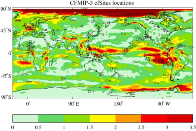
cli-Figure 2. CFMIP-3/CMIP6 cfSites locations. The contours give an indication of inter-model spread in cloud feedback from the CFMIP-2/CMIP5 amip/amip4K experiments (please refer to Webb et al., 2015a, for details).
mate regimes that contribute substantially to the inter-model spread of cloud feedbacks in climate change (Webb et al., 2015a). These outputs have so far been used to evaluate the models with in situ measurements (e.g. Nuijens et al., 2015a, b; Neggers, 2015), to investigate the diurnal cycle of cloud feedbacks (Webb et al., 2015a) and to compare cloud feed-backs in climate models with SCM and LES outputs from CGILS (Dal Gesso at al., 2015). We have added St. Helena to the list of locations in light of upcoming field work, in-creasing the total number of locations to 121 for CFMIP-3/CMIP6. A text file containing the list of locations is avail-able in the Supplement and on the CFMIP website; these are also presented graphically in Fig. 2.
For CFMIP-3 cfSites outputs are now requested for one ensemble member of the AMIP DECK experiment, and the amip-p4Kandamip-4xCO2experiments. Outputs should be provided for the full duration of each experiment. The sam-pling interval should be the integer multiple of the model time step that is nearest to 30 min and divides into 60 min with no remainder: e.g. 30 min for a 30, 15 or 10 min time step or 20 min for a 20 min time step. Outputs should be in-stantaneous (i.e. not time means) and from the nearest grid box (i.e. no spatial interpolation). We have dispensed with the cfSites outputs in the aquaplanet andamip-future4K experi-ments because these have been less widely used compared to those from the other experiments.
The cfSites outputs from CFMIP-3/CMIP6 provide instan-taneous outputs of a range of quantities (including tempera-ture and humidity tendency terms) in experiments which can be used to evaluate the present-day relationships of clouds to cloud controlling factors using in situ measurements, and at the same time explore how these relationships affect cloud feedbacks and cloud adjustments. An increasing wealth of observational data with which to evaluate the models using
these outputs is available or in the planning stage, for ex-ample from the Barbados Cloud Observatory (Stevens et al., 2015), the ARM Program (e.g. Wood et al., 2015; Marchand et al., 2015) or within the German national project on high-definition clouds and precipitation for climate-prediction, HD(CP)2, inclusive of its observational prototype experiment (HOPE), and which has collected observations over Germany following conventions adopted for CMIP (Andrea Lammert, personal communication).
CFMIP-2 also requested cloud, temperature and humid-ity tendency terms from convection, radiation, dynamics, etc. in the amip, amip4K, amipFuture and amip4xCO2, aqua-Control, aqua4xCO2 and aqua4K experiments, as global monthly mean outputs and high-frequency outputs at fixed locations (Bony et al., 2011). Upward and downward ra-diative fluxes on model levels were also requested in these experiments, and for instantaneous CO2 quadrupling in the amipexperiment only. Temperature and humidity tendency terms in particular have been shown to be useful for under-standing the roles of different parts of the model physics in cloud feedbacks (e.g. Webb and Lock, 2013; Demoto et al., 2013; Sherwood et al., 2014; Brient et al., 2015) and cloud adjustments (e.g. Kamae and Watanabe, 2012; Ogura et al., 2014) as well as in understanding clouds and circulation in the present climate (e.g. Williams et al., 2013; Oueslati and Bellon, 2013; Xavier et al., 2015). They have also been used to understand regional warming patterns such as polar ampli-fication in coupled models (e.g. Yoshimori et al., 2014).
In CFMIP-3/CMIP6 we have improved the definitions of the temperature and humidity tendency terms, and added some additional terms such as clear-sky radiative heating rates to more precisely quantify the contributions of different processes to the temperature and humidity budget changes underlying cloud feedbacks and adjustments. We have dis-pensed with the cloud water tendency terms because these have been less widely used than the temperature and humid-ity tendencies.
A shortcoming of the CMIP5 protocol was that we were unable to interpret the physical feedback mechanisms in cou-pled model experiments due to a lack of process diagnostics. For this reason in CMIP6 we are requesting these budget terms in the DECKabrupt-4xCO2experiment and the pre-industrial control as well as one ensemble member of the AMIP DECK experiment, and all of the CFMIP-3/CMIP6 experiments listed in Sects. 2.1–2.6.
effective radii/number concentrations) and a clearer diagno-sis of the roles of convective and stratiform clouds (convec-tive vs. stratiform ice and condensed water paths and cloud top effective radii/number concentrations).
3.2 COSP outputs
This section motivates and summarizes the COSP outputs requested from the DECK, CMIP6 Historical and CFMIP-3/CMIP6 experiments, as well as a corresponding set of ob-servations.
There is no unique definition of clouds or cloud types, nei-ther in models nor in observations. Therefore, to compare models with observations, and even to compare models with each other, it is necessary to use a consistent definition of clouds between the model and the satellite product in ques-tion (i.e. be “definiques-tion-aware”). Further complicating mat-ters: climate model grid boxes (typically 1◦) are much larger
than the scales over which many satellite observations are made (typically<10 km). As a result, one must downscale the climate model cloud properties to the observation scale (i.e. be “scale-aware”). The CFMIP Observation Simulator Package (COSP) enables definition-aware and scale-aware comparisons between models and multiple sets of observa-tions by producing cloud diagnostics from model simulaobserva-tions that are quantitatively comparable to a variety of satellite products from ISCCP, CloudSat, CALIPSO, MODIS, MISR and Parasol (Bodas-Salcedo et al., 2011). COSP enables a more quantitative comparison of model outputs with satellite cloud products, which often sub-sample low-level clouds in the presence of high-level clouds due to the effects of cloud overlap and attenuation (e.g. Yu et al., 1996). COSP also pro-vides histograms of various cloud properties as a function of height or pressure which are directly comparable with satel-lite products and cannot be calculated correctly from time mean model outputs. The multiple simulators within COSP allow a multi-faceted evaluation of clouds in models whereby the strengths and weaknesses of different satellite products may be considered together.
COSP is increasingly being used not only for model in-tercomparison activities, but also as part of the model de-velopment and evaluation process by modelling groups (e.g. Marchand et al., 2009; Zhang et al., 2010; Kay et al., 2012; Franklin et al., 2013; Lacagnina and Selten, 2014; Nam et al., 2014; Williams et al., 2015; Konsta et al., 2015). Many of the standard monthly and daily COSP outputs have been shown to be valuable in the CMIP5 experiments, not only for cloud evaluation, allowing a detailed evaluation of clouds and precipitation, and their interaction with radiation (e.g. Nam et al., 2012; Cesana and Chepfer, 2012; Kay et al., 2012; Klein et al., 2013; Tsushima et al., 2013; Gordon and Klein, 2014; Lin et al., 2014; Bodas-Salcedo et al., 2014; Bellomo and Clement, 2015), but also in quantifying the contributions of different cloud types to cloud feedbacks and forcing ad-justments in climate change experiments (e.g. Zelinka et al.,
2013, 2014; Chepfer et al., 2014; Tsushima et al., 2016). For a full list of studies that use COSP diagnostics for model evaluation and feedback analysis, please refer to the “CFMIP publications” section of the CFMIP website.
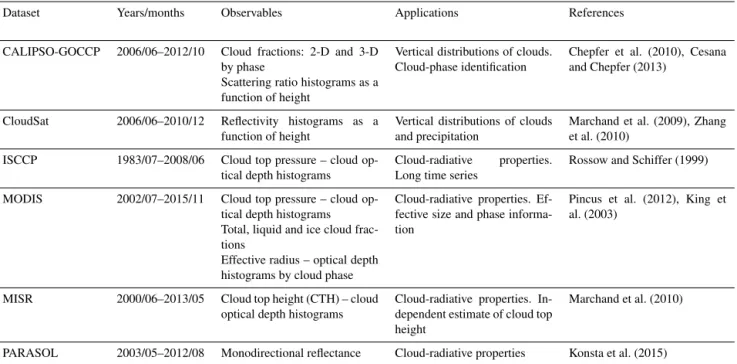
Here we will give only a brief overview of the COSP request; readers interested in the complete details of the data request are referred to the Earth System CoG website (https://www.earthsystemcog.org/projects/wip/ CMIP6DataRequest). The COSP data request for CMIP DECK and CMIP6 has been designed to span model evalu-ation across different space scales and timescales. Monthly mean diagnostics allow for the evaluation and intercom-parison of large-scale distributions of cloud properties and their interaction with radiation. High-frequency model out-puts (daily, 3-hourly) are aimed at a process-oriented evalu-ation (e.g. Bodas-Salcedo et al., 2012) and offer the oppor-tunity to exploit the synergy between multiple instruments (e.g. Konsta et al., 2015). Recent observational developments have improved our ability to retrieve cloud-radiative proper-ties. In particular, new methodologies for cloud-phase identi-fication are available for CALIPSO and MODIS, and COSP has been enhanced to provide diagnostics that are compatible with these new observational datasets (Cesana and Chepfer, 2013). These new diagnostics will help elucidate some open questions regarding the role of cloud phase in model biases (Ceppi et al., 2016; Bodas-Salcedo et al., 2016).
Within CFMIP-3/CMIP6, COSP output is requested from six simulators as follows.
– ISCCP: pseudo-retrievals of cloud top pressure (CTP) and cloud optical thickness (tau) (Klein and Jakob, 1999; Webb et al., 2001).
– CloudSat: a forward model for radar reflectivity as a function of height (Haynes et al., 2007).
– CALIPSO (Chepfer et al., 2008; Cesana and Chepfer, 2013): forward model for the lidar scattering ratio as a function of height and cloud-phase retrieval.
– MODIS: pseudo-retrievals of CTP, effective particle size and tau as a function of phase (Pincus et al., 2012). – MISR: pseudo-retrievals of cloud top height (CTH) and
tau (Marchand and Ackerman, 2010).
– PARASOL: simple forward model of mono-directional reflectance (Konsta et al., 2015).
Aerosol schemes are becoming more complex, with more elaborate representations of cloud–aerosol interactions. This makes the evaluation of the phase partitioning an important aspect of model evaluation, and height-resolved partitioning estimates from the CALIPSO simulator are included in the COSP request. Cloud phase and particle size estimates from the MODIS simulator were not available in CFMIP-2, but may prove a useful complement to investigate cloud–aerosol interactions by virtue of greater geographic sampling and longer time records. Many of the COSP diagnostics are now requested for the entire lengths of the DECK, CMIP6 Histor-ical and CFMIP-3/CMIP6 experiments to support the quan-tification and interpretation of cloud feedbacks and cloud ad-justments in a broader context. The new inclusion in this COSP request of a long time series of 3-D cloud fractions will facilitate the comparison of cloud trends with the obser-vational record (Chepfer et al., 2014). More details of all the changes with respect to CFMIP-2/CMIP5 can be found in the proposal of the CMIP6-Endorsed MIPs, available from the CMIP6 website (http://www.wcrp-climate.org/wgcm-cmip/ wgcm-cmip6).
The COSP output is in six variable groups.
– cfMon_sim: monthly means of ISCCP 2-D diagnostics (cloud fraction, cloud albedo, and cloud top pressure), ISCCP CTP-tau histogram, and CALIPSO 2-D and 3-D cloud fractions.
– cfDay_2d: daily means of ISCCP and CALIPSO 2-D diagnostics, and PARASOL reflectances.
– cfDay_3d: daily means of ISCCP and CALIPSO 3-D diagnostics.
– cfMonExtra: monthly means of CloudSat reflectitivity and CALIPSO scattering ratio histograms as a func-tion of height, CALIPSO 3-D cloud fracfunc-tions by phase, MODIS 2-D cloud fractions, MODIS CTP-tau his-togram and size-tau hishis-tograms by phase, MISR CTH-tau histograms, and PARASOL reflectances.
– cfDayExtra: daily means of CALIPSO total cloud frac-tion, MODIS CTP-tau histogram and size-tau his-tograms by phase, and PARASOL reflectances. – cf3hrSim: 3-hourly instantaneous diagnostics of
IS-CCP CTP-tau histograms, MISR CTH-tau histograms, MODIS CTP-tau histograms and size-tau histograms by phase, CALIPSO 2-D and 3-D cloud fractions, Cloud-Sat reflectitivity and CALIPSO scattering ratio his-tograms as a function of height, and PARASOL re-flectances.
The variable groups cfMon_sim and cfDay_2d are requested for all years in the amip experiment performed as part of the DECK and the CMIP6 Historical experiments, and for 140 years ofpiControl,1pctCO2, andabrupt-4xCO2. These
are requested for one ensemble member only from these experiments. They are also requested in all of the CFMIP-3/CMIP6 experiments listed in Sects. 2.1–2.6 above. cf-Day_3d is requested in one ensemble member of the DECK amipexperiment and in the CFMIP-3/CMIP6amip-p4Kand amip-4xCO2 experiments. cfMonExtra and cfDayExtra are requested for all years of one ensemble member of the AMIP DECK experiment, and cf3hrSim for the year 2008 only. (Please note that in the full data request these variable groups are in many cases split into a number of sub-tables. As noted above, the formal data request provides the definitive speci-fication of the model outputs.)
COSP is available via the CFMIP website (https://www. earthsystemcog.org/projects/cfmip). Version 1.4 is a stable code release that was made available well in advance of CMIP6 at the request of the modelling groups. Small updates are required to enable some new diagnostics requested by CFMIP-3/CMIP6, most notably joint histograms of particle size and optical thickness from the MODIS simulator; with these updates the code is known as version 1.4.1. Modelling centres are encouraged to update to COSP 1.4.1 to provide these new diagnostics, but may provide results from COSP 1.4.
Developed over the last few years, COSP 2 substantially revises the infrastructure for integrating satellite simulators in climate models. COSP 2 makes many fewer inherent as-sumptions about the model representation of clouds than do previous versions but contains an optional interface allow-ing it to be used as a drop-in replacement for COSP 1.4 or COSP 1.4.1. At the time of this writing COSP 2 is under-going final testing in two climate models. Availability of the final version will be announced on the CFMIP website and modelling groups are free to adopt it for use in CFMIP at that time.
The CFMIP community has developed a set of observa-tional datasets available via the CFMIP-OBS website (http: //climserv.ipsl.polytechnique.fr/cfmip-obs/) that are defined consistently with the COSP diagnostics and the CFMIP-3/CMIP6 data request in terms of vertical grids and time averaging periods. These are mostly reported as monthly means, although some are reported at a higher temporal res-olution for process oriented model evaluations (e.g. Kon-sta et al., 2012). Table 3 summarizes the datasets relevant to the COSP CMIP6 data request. Some of the CFMIP-OBS datasets listed in Table 3 (CALIPSO, CloudSat, ISCCP, PARASOL) are also available from the ESGF as part of the obs4MIPs project (Teixeira et al., 2014). These datasets are periodically updated to include more recent data from the rel-evant satellites, many of which are still operational. Please refer to the CFMIP-OBS website for updates.
3.3 Monthly mean diurnal cycle outputs