www.hydrol-earth-syst-sci.net/11/875/2007/ © Author(s) 2007. This work is licensed under a Creative Commons License.
Earth System
Sciences
Dynamics of resource production and utilisation in two-component
biosphere-human and terrestrial carbon systems
M. R. Raupach
CSIRO Marine and Atmospheric Research, Canberra, ACT 2601, Australia
Received: 16 June 2006 – Published in Hydrol. Earth Syst. Sci. Discuss.: 17 August 2006 Revised: 29 November 2006 – Accepted: 9 Februsray 2007 – Published: 21 February 2007
Abstract. This paper analyses simple models for “production-utilisation” systems, reduced to two state vari-ables for producers and utilisers, respectively. Two modes are distinguished: in “harvester” systems the resource util-isation involves active seeking on the part of the utilisers, while in “processor” systems, utilisers function as passive material processors. An idealised model of biosphere-human interactions provides an example of a harvester system, and a model of plant and soil carbon dynamics exemplifies a pro-cessor system. The biosphere-human interaction model ex-hibits a number of features in accord with experience, in-cluding a tendency towards oscillatory behaviour which in some circumstances results in limit cycles. The plant-soil carbon model is used to study the effect of random forc-ing of production (for example by weather and climate fluc-tuations), showing that with appropriate parameter choices the model can flip between active-biosphere and dormant-biosphere equilibria under the influence of random forcing. This externally-driven transition between locally stable states is fundamentally different from Lorenzian chaos. A be-havioural difference between two-component processor and harvester systems is that harvester systems have a capacity for oscillatory behaviour while processor systems do not.
1 Introduction
We are by now accustomed to the idea of Planet Earth as a single entity including interacting geophysical, biotic and hu-man constituent systems. Among the attributes of the earth system and its components is a propensity for autonomous dynamism. Parts of the earth system follow temporal tra-jectories which can exhibit a wide range of behaviours – growth, decay, quasi-periodic cycling, relatively sudden flips
Correspondence to:M. R. Raupach ([email protected])
between alternative states, and apparently random fluctua-tions. These dynamic behaviours are sometimes easily at-tributable to external drivers, but often they are not. Exam-ples include climate phenomena from interannual variability to ice ages; the dynamics of ecosystems, including popu-lation cycles, explosions and crashes; and the dynamics of social-ecological systems involving humans, such as boom-bust cycles and societal collapses associated with resource exploitation and depletion.
This paper focuses on the dynamical properties of parts of the earth system which are governed by the linked pro-duction and utilisation of resources. The broad aim is to identify basic system attributes which underlie commonly observed dynamical behaviours such as cycles and thresh-old transitions. For this purpose, production-utilisation sys-tems will be idealised to just two components or state vari-ables, respectively describing the producers and the utilis-ers. Within this framework, two (not always disjoint) modes for the production-utilisation interaction will be contrasted. In the first mode, resource utilisation occurs by active, often goal-seeking behaviour on the part of the utilisers; such sys-tems can be characterised as “harvester” syssys-tems. Examples include prey-predator systems and (at a high level of abstrac-tion) the biosphere-human system. In the second mode, the utilisers process resources which they receive largely pas-sively, to achieve closed material cycles (through loops in-cluding the world outside the system under study) or to pre-vent accumulation of waste in the production side of the sys-tem. Examples include water, carbon and nutrient cycling in terrestrial systems, and the production and disposal of goods in human societies. Such systems can be characterised as “processor” systems. It will be shown by example how these two modes for production and utilisation lead to different characteristic dynamical properties.
model of biosphere-human interactions is used as an exam-ple of a harvester system, and a similarly idealised model of plant and soil carbon dynamics provides a model of a pro-cessor system. The formal approach is based on the theory of dynamical systems, drawing from a well-established body of applied mathematics (e.g. Drazin, 1992; Glendinning, 1994) and particularly from applications in mathematical ecology (e.g. Gurney and Nisbet, 1998; Kot, 2001).
The plan of the paper is as follows. In Sect. 2, some nec-essary aspects of dynamical systems theory are summarised briefly. Sections 3 and 4 apply this general framework to a two-equation model of biosphere-human interactions, show-ing how even this minimal model can reproduce features of biosphere-human systems which are recognisable from qual-itative experience. In Sect. 5, a comparable analysis is made of a two-equation model for interactions between plant and soil carbon. Section 6 draws conclusions.
2 Dynamical systems theory
Consider a producer-utiliser system with two state variables (x1,x2), governed by
dx1/dt = f1(x) = g1(x)−g2(x)−k1x1
dx2/dt = f2(x) = rg2(x)−k2x2
(1)
wherex1(t )is the density of resource producers, x2(t )the
density of utilisers,g1(x)is the primary production flux into
thex1pool,g2(x)is the resource utilisation flux from thex1
pool into thex2pool,ris the efficiency for conversion ofx1
intox2,ki (i=1,2)is a first-order decay rate, andfi(x)= dxi/dt is the net input flux to the xi pool. The equations are coupled by the dependence of the fluxesg1(x)andg2(x)
on both state variables (x1,x2). The equation system can be
written in matrix form as
dx/dt = f(x) = R·g(x)−K·x x(t )=
x1(t )
x2(t )
, f(x)=
f1(x)
f2(x)
,
g(x)=
g1(x)
g2(x)
, R=
1−1 0 r
, K=
k1 0
0 k2
(2)
Models are needed for the production and utilisation fluxes,g1(x)andg2(x). For the production flux, some
com-mon possibilities are: model P0: g1(x) = p1
model P1: g1(x) = p1x1
model P2: g1(x) = p1
x1
x1+q11
model P3: g1(x) = p1
x1
x1+q11
x2
x2+q12
(3)
In model P0 the production flux g1 is constant, while in
model P1 it is proportional to the producer biomassx1. In
model P2,g1has a saturating dependence onx1of
Michaelis-Menten or Holling Type II form (Gurney and Nisbet, 1998) with scale q11, so that production depends linearly on x1
whenx1<<q11and is independent ofx1whenx1>>q11. In
model P3,g1has a saturating dependence onx1as for model
P2, together with a similar dependence on the utiliser as a symbiont,x2, with scaleq12.
For the utilisation fluxg2(x), common possibilities are
model U0: g2(x) = p2x1
model U1: g2(x) = p2x2x1
model U2: g2(x) = p2x2
x1
x1+q21
(4)
In model U0,g2is independent of utiliser level (x2) and
de-pends only on resource availability (x1). Models U1 and
U2 both assume a dependence ofg2onx2. The notation in
Eqs. (3) and (4) is thatpi is a scale for the overall magnitude of the fluxgi, andqij is a scale for the modification ofgiby state variablexj(soqijappears in the equation forgiand has the dimension ofxj).
The distinction between two-component harvester and processor systems, as characterised above, can be made for-mal through the model for g2(x). In processor systems,
where the utilisers receive recources passively,g2(x)is
in-dependent ofx2and depends only onx1(as in model U0);
in harvester systemsg2(x)depends on bothx1andx2(as in
models U1 and U2).
A particular model is specified by the parameterisa-tions for the production and utilisation fluxes from the above possibilities (or others). For instance, the well-known Lotka-Volterra equations (dx1/dt=p1x1−p2x2x1,
dx2/dt=p2x2x1−k2x2) for predator-prey dynamics (Lotka
1920; Volterra, 1926), are of the class P1U1. Several cases, including P0U1 and P2U1, are analysed by Gurney and Nis-bet (1998) and Kot (2001).
The solution of the system is a trajectoryx(t )in state (x) space, from a given initial statex(0)at timet=0, with given models forg1 andg2and with given parameters (r,ki,pi, qij,. . . ). Much of the behaviour of this solution is determined by the equilibrium points (xQ, denoted by a superscriptQ) at whichdx/dt=f(x)=0, and by the local stability of the trajec-tories around these points (Drazin, 1992; Glendinning, 1994; Casti, 1996, 2000). The existence of equilibrium points is governed by the nonlinear equation
fxQ = R·gxQ − K·xQ = 0 (5)
which is satisfied whenxQis an equilibrium point. The sta-bility ofxQis determined by the linearised system
dx′/dt = J·x′ (6)
have negative real parts, thenxQis stable (so that trajectories nearxQconverge toxQast → ∞), and if at least oneλihas a positive real part, thenxQis unstable (so that an infinitesi-mal disturbance fromxQcauses trajectories to diverge from
xQast→∞). The imaginary parts ofλi determine whether the solutions nearxQhave oscillatory components.
For the two-dimensional system of Eq. (1), the Jacobian is (with∂jgi=∂gi/∂xj):
J =
∂1g1−∂1g2−k1 ∂2g1−∂2g2
r∂1g2 r∂2g2−k2
(7) For this (or any) two-dimensional system, the characteristic equation for the eigenvalues ofJis
λ2 − (TrJ) λ + (DetJ) = 0 (8) It is well known (Drazin 1992 p. 170–176) that for two-dimensional systems the main options for the stability of an equilibrium pointxQare as follows: if both roots (λ1,2) of
Eq. (8) are real and negative (positive), then xQ is a sta-ble (unstasta-ble) node: nearby trajectories converge to (diverge from)xQalong non-spiralling curves. If both rootsλ1,2are
complex with negative (positive) real parts, thenxQis a sta-ble (unstasta-ble) focus or spiral point: nearby trajectories spiral inward to (outward from)xQ. If the rootsλ1,2have real parts
of opposite sign, thenxQ is a saddle point: nearby trajec-tories are hyperbolic. A saddle point is unstable in general, except for approach along particular directions. These con-ditions are equivalent to the following:
xQis stable if (DetJ) >0 and(TrJ) <0
xQis unstable if (DetJ) >0 and(TrJ) >0
xQis a saddle if (DetJ) <0
(9)
The spiral (oscillatory) tendency of the local trajectories aroundxQis determined by the discriminant (D) of the left side of Eq. (8):
D >0 (stable node: nonspiral) D <0 (stable focus: spiral) with D=(TrJ)2−4 DetJ
(10)
For two-component processor systems as defined above, ∂2g2=0 and D=(∂1g1−∂1g2−k1+k2)2+4(∂1g2)(∂2g1)r.
Provided ∂1g2≥0 and ∂2g1≥0, as in all examples above,
D is positive. In these conditions, oscillatory (spiralling) behaviour is not possible.
3 Biosphere-human interactions: basic model
As an example of a producer-utiliser system of the har-vester type, we consider a minimal model of biosphere-human interactions in which the biosphere acts as producer and humans as utilisers. The interaction between humans and the natural biosphere that sustains them clearly involves a vast range of biophysical, economic, social and cultural
processes which together have shaped human populations diverse ways determined by both biogeographical circum-stances and contingent history (Flannery, 1994; Diamond, 1991, 1997, 2005). It goes without further emphasis that a two-equation model cannot capture even a fraction of this richness. Nevertheless, even such a simple model is capable of discerning some broad patterns.
The state variables are the biomassb(t )and human pop-ulationh(t )in a specified region. We first consider a very simple formulation in whichb(t )andh(t )are governed by
db/dt = p−cbh−kb (11)
dh/dt = r(cbh−mh) (12)
wherepis a constant primary biomass production flux,cthe rate of extraction of biomass per human; k the rate of de-cay of biomass by respiration,mthe maintenance biomass requirement per unit time per human, and r the fractional growth rate of human population per unit biomass surplus. The model assumes that the growth rate ofhdepends on the difference(cbh−mh)between the extraction of biomass by harvest (cbh) and the biomass per unit time required to main-tain the human population (mh). This difference is a surplus production measured in biomass units, leading to population increase (decrease) at raterwhen the surplus(cbh−mh)is positive (negative). This model is a special case of Eqs. (1) to (4) with production and harvest models of the class P0U1 and variable substitutions (x1, x2)→(b, h), (g1, g2)→(p, cbh),
and(k1, k2)→(k, rm). Assumptions in this highly
simpli-fied model are that there is no transfer of eitherborhacross the boundaries of the model region, and also that biomass production (p) does not depend directly onh, for instance by technological innovation (see Wirtz and Lemmen (2003) for a model in which there is a dependence ofponh).
Given its idealisations and restrictions, the model can be interpreted in two ways. First, b and h can be regarded strictly as biomass and human population, respectively. This view is relevant to interactions between isolated, homoge-neous human populations and their environments. A second, broader view regardsbas “renewable natural capital” andh as “human capital”. In this case the model may have some applicability to technologically advanced societies where in-crease in human capital continues unchecked even though human populations are stabilising or declining. In the con-text of farm management, a model with some similarities to the present (b, h)model has been proposed by Fletcher et al. (2006), withbandhinterpreted in this way.
0.2 0.4 0.6 0.8 1 1.2 b 0.1
0.2 0.3 0.4 0.5 0.6
h vary c
0.2 0.4 0.6 0.8 1 1.2 b 0.1
0.2 0.3 0.4 0.5 0.6
h vary r
0.2 0.4 0.6 0.8 1 1.2 b 0.2
0.4 0.6 0.8 1
h vary p
0.2 0.4 0.6 0.8 1 1.2 b 0.2
0.4 0.6 0.8 1
h vary m
Fig. 1.Trajectories(b(t ), h(t ))of the basic biosphere-human model on thebhplane, with different curves showing variation of (top left) primary productionp; (top right) human maintenance requirement
m; (bottom left) extraction ratec; (bottom right) growth rater. The centre case (black curve, identical in all plots) has parametersp=1,
k=1,m=2,c=4,r=1. In each plot, the varied parameter takes log-arithmically spaced values from 0.4 to 2.5 of its centre-case value (rainbow curves, red to violet). All trajectories have initial condition
(b(0), h(0))=(1,0.1). Note that the ordinate scale differs between panels.
can be defined as U = km
cp, V = rm
k (13)
Equations (11) and (12) have two equilibrium points (de-noted A and B), given by:
Point A: bQA=p/ k, hQA=0
Point B: bQB =m/c, hQB =(p/m)−(k/c) (14) These points have the following properties.
1. Point A, the biosphere-only equilibrium, occurs in the absence of humans (h=0), when the biosphere equili-brates to a biomassbQA=p/ kat which production (p) balances respiration (kb). Point A is a saddle point with its stable axis along the lineh=0 (Appendix A). 2. As soon ash exceeds zero for any reason, the system
leaves point A and approaches point B, the equilibrium for coexistence of a human population with the bio-sphere. Point B is always a stable equilibrium point (Appendix A). It is a stable focus (spiral trajectories) whenV >(4U (1−U ))−1, and a stable node (non-spiral trajectories) otherwise.
3. Production (p) determines the equilibrium biomass at point A (bQA), but at point B,pinstead determines the equilibrium human population (hQB). The biomass at point B (bQB) is independent ofpand is determined by mandc, attributes of the human population.
4. Points A and B are both independent of the growth rate rand therefore of the groupV. The role ofr(andV) is to determine the nature of the approach to point B, as illustrated below.
5. For hQB to be positive, the parameters must satisfy 0<U <1.
A “resource condition index”W can be defined as the ratio of the equilibrium biomass values with and without human utilisation:
W = b QB
bQA (15)
In the presence of a human population at equilibrium, a fractionW of the potential (unutilised) biomass remains in place, and a fraction(1−W )is removed by utilisation. Equa-tions (13) and (14) show that for the basic system governed by Eqs. (11) and (12), we haveW=U. (In an extended ver-sion of this model considered below,W is a function ofU). The fractional human appropriation of net primary produc-tion, or HANPP (Boyden, 2004), is g2/g1=cbh/p, which
for the basic model at equilibrium point B is 1−U=1−W. Figure 1 illustrates the system dynamics by plotting trajec-tories(b(t ), h(t ))on thebhplane under four scenarios, re-spectively corresponding to variation ofp,m,candrabout a centre case withp=1,k=1,m=2,c=4,r=1. The total range for the varied parameter is about a factor of 5 in each case. The initial condition is that the biomass takes the potential valuebQA(= 1 with the centre-case parameter choices) with a small human population.
– Scenario 1 (variation of p): As p (the primary pro-duction of biomass) increases, the system responds through an increase in the equilibrium human popu-lation (hQB=p/m−k/c), not the equilibrium biomass (bQB=m/c), as noted above. For low values ofp, the dimensionless groupU exceeds 1 and the coexistence equilibrium (point B) is no longer viable as it is both unphysical (hQB<0) and also unstable, so the system reverts to the biosphere-only equilibrium (point A). This occurs at different points along thebaxis under varia-tion ofp, sincebQA=p/ k.
– Scenario 2 (variation of m): One might expect that de-creasing the human maintenance requirementmwould cause the human population to “walk more lightly upon the land”, increasing the equilibrium resource condition indexW. However, the reverse is the case: decreasing mdecreasesW, increases the equilibrium human pop-ulation rapidly, and decreases the equilibrium biomass. With decreasingmthere is a decreasing tendency of tra-jectories to spiral, and lowmvalues are associated with nodes (non-spiral trajectories near equilibrium point B).
the intensity of human exploitation of the biosphere. In-creasingccauses the equilibrium biomass to decrease (as might be intuitively expected) but the human popu-lation increases only slowly. Also, ascincreases, there is an increase in the amplitude of oscillations associated with spiral orbits. The qualitative insight provided by this scenario is that more aggressive resource extraction has the counter-intuitive effect of decreasing the equilib-rium biomass while not increasing the equilibequilib-rium hu-man population by anything like as much. Equation (14) shows that asc→∞, hQB approaches the upper-limit value ofp/mwhilebQB approaches zero. In this limit the biomass is over-exploited without a return in the form of a high human population as in Scenario 2.
– Scenario 4 (variation of r): Under variation of the growth rate of the human population per unit biomass surplus, equilibrium point B does not change (see prop-erty 4, above) but there is an increase in the amplitude of the decaying oscillations with which the system ap-proaches this point. Hence, increase ofr increases the tendency of the system to exhibit “boom-bust” oscilla-tions. A similar trend is evident with increasingc, al-though in that case there is also a shift in the equilibrium point as noted in the previous paragraph.
The oscillatory behaviour of this simple model (especially at high cand r values) echoes the hypothesis of Flannery (1994) that when humans move into a previously unoccu-pied ecosystem, the biosphere-human system undergoes an initial rapid exploitation phase, a resource crash accompa-nied by rapid decrease in the human population, and finally an equilibration.
4 Biosphere-human interactions: extended model
4.1 Model formulation
The above basic two-equation model of biosphere-human in-teractions is open to several criticisms (other than those as-sociated with the extreme idealisation to just two state vari-ables). Two of the main ones are: (1) the primary produc-tionpis assumed to be constant at all levels of the biomass b, whereas production is actually limited (approximately lin-early) bybat lowb, and saturates to a constant value at high b; and (2) the harvest fluxcbhis assumed in the basic model to be resource (b) limited at all resource levels, so there is no resource level (no matter how large) at which the harvest flux saturates with respect tob. To investigate the effect of these possible limitation and saturation attributes of the pro-duction and harvest fluxes, we extend the basic model from class P0U1 to class P2U2.
The extended model is db
dt = p
b
b+bP
− kb − cbh
b
H b+bH
(16) dh
dt = rcbh
bH
b+bH
− rmh (17)
wherebP andbH are respectively the biomass scales for re-source saturation of production and harvest. The factors in brackets, accounting for resource saturation, are written in a form which keeps the dimensions ofp,c,k,mandr the same as in the basic model. AsbP→0 andbH→∞, these factors approach 1 and Eqs. (16) and (17) revert to Eqs. (11) and (12).
The model now has seven dimensional parameters (p,c, k,m,r,bP,bH) and three dimensions ([B], [H], [T]). Hence there are four independent dimensionless groups. With this many parameters, analysis is greatly helped by normalising the model rigorously to a dimensionless form. (This was not done in the foregoing analysis of the basic model; the di-mensionless approach provides a more concise description at the expense of the need for careful interpretation when pa-rameters appear in both dimensionless groups and scales, as illustrated below). Dimensionless versions of the model vari-ablesb,handt are defined asx1=b/bscale,x2=h/ hscaleand
s=t /tscale, wherebscale,hscaleandtscaleare scales to be
con-structed from the externally specifed parameters. They are chosen as follows: bscale is the equilibrium biomass in the
absence of a human population,bscale=bQA=(p/ k)−bP, so thatx1=1 for the equilibrium biosphere without utilisation;
hscale is set as hscale=rbscale, becauser is the obvious
pa-rameter with dimension [H B−1] for relating the scales for handb; andtscaleis chosen as 1/ k, the intrinsic biospheric
time scale. With these choices, the dimensionless biomass, human population and time are
x1=
b p/ k−bP
, x2=
b r(p/ k−bP)
, s=kt (18) The four independent dimensionless groups are chosen as
U= m
cbQA, V = rm
k , a1= bP
bQA, a2= bQA
bH (19)
The definition of U reverts to that for the basic model (Eq. 13) as bP→0, and the definition ofV is identical to that for the basic model. Substituting these dimensionless variables into Eqs. (16) and (17), the dimensionless form of the extended model is found to be:
dx1
ds =
(1+a1)x1
x1+a1 −
x1 −
V x1x2
U (1+a2x1)
(20) dx2
ds =
V x1x2
U (1+a2x1) −
V x2 (21)
0.5 1 1.5 2 x1 0.2
0.4 0.6 0.8 1 1.2
g1
Fig. 2. Production term in the dimensionless extended biosphere-human model,g1(x1)=(1+a1)x1/(x1+a1), plotted againstx1for a1ranging from 0 to 1.
0.2 0.4 0.6 0.8 1
x1 0.2
0.4 0.6 0.8 1 x2
0.5 1 1.5 2 a2
0.2 0.4 0.6 0.8 1 Umax
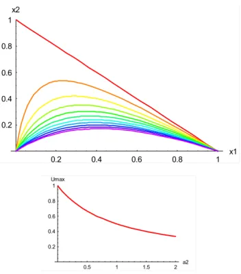
Fig. 3. (top) Coexistence equilibrium(x1QB, x2QB)for the dimen-sionless extended biosphere-human model withV=1, plotted on the
x1x2plane withWvarying parametrically from 0 to 1 along each
curve (left to right) anda1varying from 0 to 1 across curves (red: a1=0; violet;a1=1). (bottom)Umax=1/(1+a2)as a function of a2.
anda2→0. The reason for defining a2 as proportional to
1/bH rather thanbH is that it is more convenient to take the zero than the infinite limit in computations.
The production term in Eq. (20), g1(x1) =
(1+a1)x1/(x1+a1), is plotted against x1 in Fig. 2 for a
range ofa1values. The choicea1=0 gives constant
produc-tion (g1=1), while all other choices give a resource-limited
production withg1=0 atx1=0 andg1=1 atx1=1.
4.2 Equilibrium points
Equations (20) and (21) have three equilibrium points at whichdx1/ds=0 anddx2/ds=0:
Point Z: (x1QZ, xQZ2 )=(0,0) Point A: (x1QA, xQA2 )=(1,0)
Point B:
x1QB =1 U
−a2U
x2QB = U (1−a2U−U )
V (1−a2U )(a1(1−a2U )+U )
(22)
Points A and B are respectively a biosphere-only equilibrium and a biosphere-human coexistence equilibrium, similar to those for the basic model (Eq. 14). Point Z is an additional equilibrium point at the origin, with biomass and human pop-ulation both zero. Evaluation of the resource condition index W, defined by Eq. (15), gives
W =x QB
1
x1QA = U 1−a2U
, U = W
1+a2W
(23)
Hence, for the extended model,Wis a function of the dimen-sionless groupU, in contrast with the basic model for which W=U. SubstitutingW forU in Eq. (22), equilibrium point B can be written in the alternative, simpler form
x1QB =W, x2QB = W (1−W ) V (a1+W )
(24) Biophysically realistic equilibrium solutions can only ex-ist in a subset of parameter space. First, all parameters must be non-negative. Second, for the biosphere-only equi-librium biomass (bQA) to be positive, it is necessary that bscale>0, which requires that (p/ k)>bP. This is a con-dition on the dimensional parameters which becomes im-plicit when the model is made dimensionless, being incor-porated into a requirement onbscale. Third, the equilibrium
biomass in a harvested system cannot exceed the equilib-rium biomass without harvest, so biophysically realistic so-lutions at equilibrium point B exist only whenW is between 0 and 1. From Eq. (23), this means that 0<U <Umax, where
Umax=1/(1+a2). This is the counterpart for the extended
model of the requirement 0<U <1 for the basic model. Figure 3 shows the behaviour of equilibrium point B on thex1x2plane in response to variation of the parametersa1
(which varies 0 to 1 across curves) andU(which varies para-metrically along each curve from 0 toUmax). This variation
of U means that W varies from 0 to 1 along each curve. The curves do not change asa2 is varied, but the
paramet-rically varying U values along each curve change witha2
because of the dependence of Umax on a2, shown in the
Fig. 4. Flow fields onx1x2plane for the dimensionless extended
biosphere-human model, with V=1, a1=a2=0.5, and W=0.2 (top), 0.5 (middle) and 1.0 (bottom). Thex1(horizontal) axis
ex-tends from 0 to 1.2, and thex2(vertical) axis from 0 to 0.5.
to shrink (stretch) the vertical axis. The most important as-pect of this figure is the change in the behaviour of equi-librium point B in the transition from the basic model (with constant production anda1=0) to the extended model (with
biomass-limited production anda1>0). As resource
condi-tion declines (W→0 orU→0), the human population in the basic model increases (x2QB→1/V,hQB→(k/m)bQB), but in the model with biomass-limited production,x2QBandhQB both decline (more realistically) to zero.
4.3 Trajectories
A first glimpse into the dynamical behaviour of the ex-tended model is provided in Fig. 4, in which the flow vector (f1(x1, x2), f2(x1, x2))=(dx1/ds, dx2/ds)is plotted on the
x1x2plane for three differentWvalues, 0.2, 0.5 and 1 (other
parameters areV=1,a1=0.5,a2=0.5). ForW=0.2 and 0.5,
the oscillatory nature of the flow around equilibrium point B is clear. ForW=1, point B coincides with point A, the biosphere-only equilibrium.
0.2 0.4 0.6 0.8 1x1 0.1
0.2 0.3 0.4 0.5
x2 vary a1 from 0. to 2.
0.2 0.4 0.6 0.8 1x1 0.1
0.2 0.3 0.4 0.5
x2 vary a2 from 0. to 2. 0.2 0.4 0.6 0.8 1x1
0.1 0.2 0.3 0.4 0.5
x2 vary w from 0.1 to 1.
0.2 0.4 0.6 0.8 1x1 0.1
0.2 0.3 0.4 0.5
x2 vary v from 0.5 to 2.
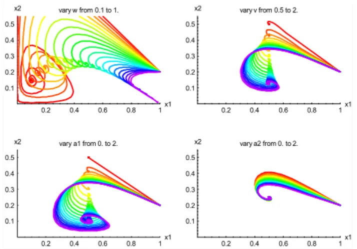
Fig. 5. Trajectories onx1x2plane for the dimensionless extended
biosphere-human model, with centre-case parameters W=0.5,
V=1, a1=0.5, a2=0.5. The initial condition is alwaysx1=1.0,
x2=0.2. Panels show (with colours proceeding through the rain-bow from red to violet) the effect of(a)variation ofWfrom 0.1 to 1;(b)variation ofV from 0.5 to 2;(c)variation ofa1from 0 to 2; (d)variation ofa2from 0 to 2.
Figure 5 shows the response of trajectories to variation (in turn) of W, V, a1 anda2 around the centre caseW=0.5,
V=1, a1=0.5 and a2=0.5. This is a high-level summary
of the response of the system to changes in external condi-tions, but it needs care in interpretation because dimensional parameters (p,c,k,m,r,bP,bH) affect both the dimension-less groups (W orU,V,a1anda2) and also the normalising
scales (bscale,hscaleandtscale). To infer the response of
di-mensional state variables (bandh) to changes in dimensional external parameters with Fig. 5 and similar dimensionless plots, it is necessary to consider the influences of the dimen-sional parameters both on the dimensionless groups and also on the scales with which the axes in Fig. 5 are normalised. Keeping this in mind, the implications of Fig. 5 are as fol-lows.
– Variation ofW: Since W is a function ofU through Eq. (23), variation ofW from 0 to 1 occurs asUvaries from 0 toUmax. As this occurs, the equilibrium point
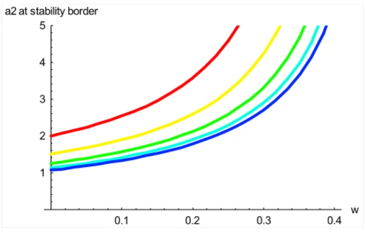
0.1 0.2 0.3 0.4 w 1
2 3 4 5
a2 at stability border
Fig. 6. Instability threshold for the coexistence equilibrium point of the dimensionless extended biosphere-human model as a func-tion ofa1,a2andW. Curves show the instability threshold on the (W, a2)plane, witha1=1, 2, 4, 8, 16 (red to blue). Points above the curves are unstable.
0.2 0.4 0.6 0.8 1x1 0.2
0.4 0.6 0.8 1
x2 vary w from 0.3 to 0.1
0.2 0.4 0.6 0.8 1x1 0.2
0.4 0.6 0.8 1
x2 vary a2 from 1 to 4
Fig. 7. Trajectories onx1x2plane for the dimensionless extended biosphere-human model illustrating the effect of crossing the insta-bility threshold for the coexistence equilibrium (point B). Centre-case parameters areW=0.2,V=0.1,a1=2,a2=2. Left panel: two trajectories withW=0.3 and 0.1 and other parameters at centre-case values. Right panel: two trajectories witha2=1 and 4, and other pa-rameters at centre-case values. In each case the first (red) trajectory is stable, and the second (blue) trajectory is unstable, entering a limit cycle.
– Variation ofV:This variation reflects essentially a vari-ation in the growth rater. AsV increases the oscillatory tendency of the model increases, as for the basic model (Fig. 1). With increasing V there is also a decrease inxQB2 , the equilibrium dimensionless hQB, whereas the equilibrium point (bQB, hQB) for the basic model is independent ofr andV (see Scenario 4 for the basic model). The apparent difference arises because r ap-pears in the normalisation ofhQBtox2QB (see Eq. 18).
– Variation ofa1:Increasinga1occurs with increase ofbP
and thus the limitation of production at low biomass and saturation at high biomass (Fig. 2). This has a strong tendency to increase the oscillatory behaviour of the model, and also causes a reduction in x2QB, the equi-librium dimensionlesshQB, whilex1QB stays constant (a trend also evident in Fig. 3).
– Variation ofa2:Increasinga2occurs with progressively
more saturation of the harvest flux at high biomass, and with decreasingbH. For the parameter range shown in Fig. 5, increase ina2causes a mild decrease in the
os-cillatory tendency of the trajectories while leaving the equilibrium point (x1QB, x1QB) unchanged.
4.4 Stability
The stability of the equilibrium points for the extended model is more subtle than for the basic model, for which the co-existence equilibrium (point B) is stable for all parameter choices. Stability analysis for the extended model leads to the following conclusions (see details in Appendix B).
– Equilibrium point Z (the origin) is a saddle point with its stable axis oriented along thex2axis, so point Z is
un-stable with respect to an infinitesimal variation inx1and
stable with respect to a variation inx2. Hence a small
positive perturbation in biomass from point Z causes the biosphere to move away from point Z and approach point A, whereas a small human population dies out as it has nothing to live on.
– Point A (the biosphere-only equilibrium) is a saddle point with its stable axis in thex1 direction, as in the
basic model. In the absence of humans, the biosphere approaches point A along thex1axis from either
direc-tion. A small positive perturbation inhorx2causes the
system to leave point A and approach point B.
– Point B (the coexistence equilibrium) can be either sta-ble or unstasta-ble, depending on values ofW,a1anda2.
The condition for stability of point B is (see Appendix B): Y >0 (stable)
Y <0 (unstable)
with Y =1+a1−a1a2+2a1a2W+a2W2
(25)
Hence, for givenW anda1, instability occurs whena2
ex-ceeds a threshold value: a2 > a2Thresh =
1+a1
a1−2a1W −W2
(26) This threshold value is plotted on the (W,a2) plane in Fig. 6,
for several values ofa1. Instability occurs whenW is low
anda2anda1are high. Figure 7 shows how the system
be-haviour changes asW anda2cross this threshold. When the
parameters are on the stable side of the threshold, trajectories are attracted to point B, but for parameters on the unstable side of the threshold, trajectories are repelled from point B and enter a limit cycle in which oscillatory behaviour of the system does not die away but continues for all time.
(resource-limited production and utilisation) forms. First, the basic model has biosphere-only and coexistence equilibrium points, but the extended model has an additional equilibrium point at the origin. Second, with declining resource condi-tion (W), h increases in the basic model but (more realis-tically) declines toward zero in the extended model. Third, the extended model is more prone to strong oscillatory be-haviour than the basic model, especially at lowW. Fourth, in the basic model the coexistence equilibrium is always stable, but in the extended model it becomes unstable at lowW and with strong resource limitation of production and/or utilisa-tion (largea1ora2). In these conditions, trajectories enter a
limit cycle of orbits about the coexistence equilibrium point, rather than eventually reaching it.
5 Plant and soil carbon dynamics
Carbon dynamics in the plant-soil system provides an ex-ample of a producer-utiliser system which operates in pro-cessor mode, as defined in the introduction. The producers are plants, through the assimilation of atmospheric CO2into
biomass, and the utilisers are soil heterotrophic organisms which feed off plant litter and respire the carbon back to the atmosphere as CO2.
5.1 Model formulation
The system is modelled using an idealised, two-equation rep-resentation with state variables for the stores of biomass car-bon (x1)and litter and soil carbon (x2). The governing
equa-tions are: dx1
dt = F (t )
x
1
x1+q1
x2
x2+q2
+s1−k1x1 (27)
dx2
dt = k1x1−k2x2 (28)
whereF (t )is a forcing term describing the net primary pro-duction (NPP);q1andq2are scales for the limitation of
pro-duction by lack ofx1andx2, respectively;k1andk2are rate
constants for the decay ofx1andx2, respectively; ands1is a
component of the primary production which is independent of bothx1andx2. We consider both the case whereF (t )is
independent of time,F (t )=F0, and also the case whereF (t )
is a random function of time. The model parameters areq1,
q2,k1,k2, ands1, together withF0or parameters
character-isingF (t )as a random function.
These equations are a simplification the carbon dynamics in typical terrestrial biosphere models, including models of global vegetation dynamics as in the DGVM intercompari-son of Cramer et al. (2001), and the terrestrial biosphere com-ponents of coupled carbon-climate models as in the C4MIP intercomparison of Friedlingstein et al. (2006). Character-istics of such terrestrial biosphere models at several levels
of complexity are reviewed by Raupach et al. (2005). Rela-tive to sophisticated terrestrial biosphere models, Eqs. (27) and (28) are an extreme idealisation: all biomass carbon (leaf, wood, root) is lumped into a single storex1governed
by an equation of the form dx1/dt=(NPP)–(litterfall), and
all litter and soil carbon into a single store x2 governed
bydx2/dt=(litterfall)–(heterotrophic respiration). Litterfall
and heterotrophic respiration are parameterised as first-order decay fluxes, k1x1 and k2x2. NPP is assumed to depend
on three factors: (1) a forcing term F (t ) representing the fluctuating availability of light and water resources through weather and climate variability, (2) a factorx1/(x1+q1)of
Michaelis-Menten form describing the limitation of NPP by lack of biomass in resource-gathering organs (leaves, roots), and (3) a factorx2/(x2+q2), also of Michaelis-Menten form,
describing the integrated symbiotic effects of soil carbon on plant productivity. This symbiotic factor accounts for the overall beneficial effect of soil carbon on plant growth, through processes such as nutrient cycling and improvement in soil water holding capacity (often not included in sophisti-cated terrestrial biosphere models such as those surveyed in the references above). The parameters1represents a (small)
production term that is not dependent onx1andx2, for
ex-ample generation of biomass from a long-term reservoir of seed propagules. For the present purpose,s1 is assumed to
be a constant flux independent of external conditions as well asx1andx2.
Equations (27) and (28) are identical to the test model used in the OptIC (Optimisation Intercomparison) project (Trudinger et al., 2007; also http://www.globalcarbonproject. org). The aim of OptIC is to compare several model-data synthesis (parameter estimation and model-data assimilation) approaches for determining parameters in biogeochemical models from multiple sources of noisy data. Equations (27) and (28) are used as a simple test model which embodies features of a real biogeochemical model, together with gen-erated data from model forward runs with added noise, for which “true” parameters are known.
5.2 Equilibrium points and stability
We consider first the situation with steady forcing,F (t )=F0.
Seeking the equilibrium points pointsxQat whichdx1/dt=
dx2/dt= 0, Eq. (28) shows that
x2Q=x1Qk1/ k2 (29)
and Eq. (27) implies thatx1Qsatisfies the cubic equation j (x1)=c0+c1x1+c2x12+c3x13=0
c0
c1
c2
c3
=
q1q2k2s1/k21
((q1k1+q2k2)s1−q1q2k1k2)/ k21
(F0−q1k1−q2k2+s1)/ k1
−1
1 1 2 3 4 x1
8 6 4 2 2 4 6 8 j
0.1 0.1 0.2 0.3 0.4x1
0.04 0.02 0.02 0.04 0.06 0.08 0.1 j
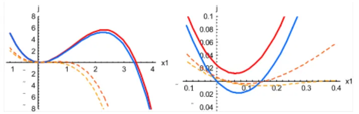
Fig. 8. The cubicj (x1)defined by Eq. (30), with reference-case
parameter valuesF0=1,q1=1,q2=1,k1=0.2,k2=0.1,s1=0.01. Solid red and blue lines show the effect of varying s1 (red: s1=0.01; blue: s1=0, with other parameters at reference-case val-ues). Dashed orange (heavy) and yellow (light) lines show effect of varyingk1(orange: k1=0.4; yellow: k1=0.5, with other
parame-ters at reference-case values). Left panel shows all zeros ofj (x1).
Right panel is an expanded view showingj (x1)near the origin.
Thus the equilibrium points are of the form
xQ=(x1Q, x1Qk1/ k2), where x1Q is a solution of the
cu-bic equationj (x1Q)=0. This equation has either one or three real roots, yielding either one or three equilibrium points. At least one root must be positive (x1Q>0) for a nontrivial, biophysically meaningful solution to exist. The cubicj (x1)
is plotted in Fig. 8 with reference-case parameters F0=1,
q1=1, q2=1, k1=0.2, k2=0.1 (the red curve; other curves
are described below).
When the equilibrium points are determined by the roots of a single equation, it is not necessary to appeal to the Ja-cobian and its characteristic equation to determine stability. A sufficient criterion is that an equilibrium pointx1Qis sta-ble ifdj/dx1<0 at x1=x1Q, and unstable otherwise. Since
j (x1)=−x13+. . ., it is clear from the geometry (see Fig. 8)
that if there is just one equilibrium point then it is stable, whereas if there are three equilibrium points, say A, B, C with equilibriumx1valuesx1QA,xQB1 andx1QCin increasing
order, thenxQA1 andx1QCare stable andx1QBis unstable. For all biophysically admissible parameter choices,j (x1)has at
least one stable root with x1>0. This will be designated
asx1QC, the largest stable equilibrium value of x1, and can
be identified as a “healthy” or “active” equilibrium state of the system. It is important to understand whether and when there is another biophysically attainable and stable equilib-rium state, equilibequilib-rium point A, withx1QA≥0. This depends on the parameter choices, particularly fors1. There are three
main possible kinds of behaviour, as follows.
1. Ifs1>0 and the cubic j (x1) crosses the x1 axis only
once, then there is only one equilibrium pointx1QC, the “active-biosphere” point. It is always stable, so the sys-tem must approach it under steady forcing. This is the outcome with the reference-case parameters, as shown by the red curve in Fig. 8.
2. Ifs1>0 and j (x1)crosses thex1axis three times, all
greater than zero, then there are two stable, positive equilibrium points (xQA1 andx1QC)on either side of one unstable point (xQB1 ). The two dashed curves in Fig. 8 show this outcome occurring as k1 is increased from
0.2 to (respectively) 0.4 and 0.5, with other parame-ters held at reference-case values. In this case, xQC1 is the “active-biosphere” point as before, andx1QAis a “dormant-biosphere” equilibrium.
3. If s1=0, then there is a stable equilibrium point (A)
of Eqs. (27) and (28) at the origin, in addition to the “active-biosphere” equilibrium pointx1QC>0. (Ex-istence of this root is assured because s1=0 implies
c0=0, sox1Q=0 is a root ofj (x1); stability follows
be-cause dj/dx1=c1 atx1=0, and when s1=0, we have
c1= −q1q2k2/ k1, which is negative for positive values
ofq1,q2,k2). The equilibrium point at the origin
cor-responds to “extinction” of the biosphere in this simple model system, since once the system reaches the origin withs1=0, it remains there for all subsequent time, no
matter what the forcingF (t ). The blue curve in Fig. 8 shows this case.
In addition to these three options, there are other possibil-ities. For some parameter combinations the cubicj (x1)has
no positive or zero solutions (that is, all crossings of thex1
axis occur whenx1<0), so these parameter combinations are
not biophysically realisable. Also, ifs1=0 and eitherq1=0
orq2=0, the model relaxes to a simpler form asj (x1)is of
lower degree than a cubic. In these cases there can be only one stable equilibrium point.
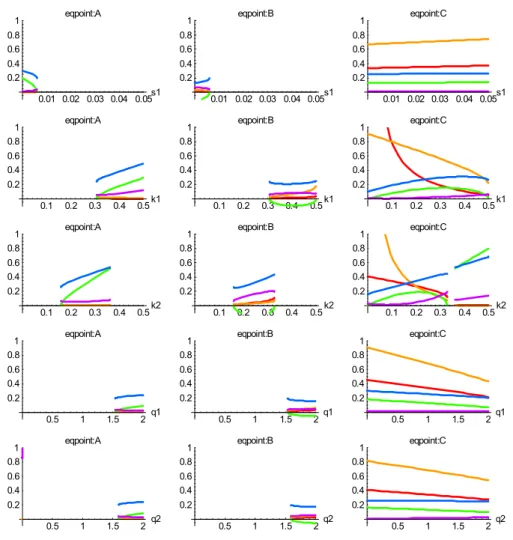
Figure 9 shows how the three main kinds of behaviour can all arise as parameters are varied around the reference case. Each panel of this figure superimposes plots of x1Q (red),x2Q(orange), DetJ(green),−TrJ(blue) and the dis-criminant(D=(TrJ)2−4 DetJ), at a particular equilibrium point (A, B, C, in different columns), and examines the re-sponse of these quantities to variation of a parameter (s1,k1,
k2, q1, q2, in different rows). No lines are plotted where
real equilibrium solutions do not exist. The trace and the de-terminant of J show the stability of the point, since Det J
and−TrJmust both be positive for stability, from Eq. (9). The discriminant shows whether local trajectories around the point are non-spiral or spiral, from Eq. (10). The picture is rich: the “active-biosphere” equilibrium point C exists as a stable node (non-spiral trajectories) for nearly all parameter choices. Points A and B form a pair, in that neither exists or both exist. When both exist, point A is always stable and point B always unstable. The discriminant is always posi-tive where points exist, indicating that spiral behaviour is not observed in this model over the slices of parameter space sur-veyed in Fig. 9.
0.5 1 1.5 2 q2 0.2
0.4 0.6 0.8
1 eqpoint:A
0.5 1 1.5 2q2
0.2 0.4 0.6 0.8
1 eqpoint:B
0.5 1 1.5 2q2
0.2 0.4 0.6 0.8
1 eqpoint:C
0.5 1 1.5 2 q1
0.2 0.4 0.6 0.8
1 eqpoint:A
0.5 1 1.5 2q1
0.2 0.4 0.6 0.8
1 eqpoint:B
0.5 1 1.5 2q1
0.2 0.4 0.6 0.8
1 eqpoint:C
0.1 0.2 0.3 0.4 0.5k2
0.2 0.4 0.6 0.8
1 eqpoint:A
0.1 0.2 0.3 0.4 0.5k2
0.2 0.4 0.6 0.8
1 eqpoint:B
0.1 0.2 0.3 0.4 0.5k2
0.2 0.4 0.6 0.8
1 eqpoint:C
0.1 0.2 0.3 0.4 0.5k1
0.2 0.4 0.6 0.8
1 eqpoint:A
0.1 0.2 0.3 0.4 0.5k1
0.2 0.4 0.6 0.8
1 eqpoint:B
0.1 0.2 0.3 0.4 0.5k1
0.2 0.4 0.6 0.8
1 eqpoint:C
0.01 0.02 0.03 0.04 0.05s1
0.2 0.4 0.6 0.8
1 eqpoint:A
0.01 0.02 0.03 0.04 0.05s1
0.2 0.4 0.6 0.8
1 eqpoint:B
0.01 0.02 0.03 0.04 0.05s1
0.2 0.4 0.6 0.8
1 eqpoint:C
− −
Fig. 9. Variation ofxQ1/10 (red),x2Q/10 (orange), 10 DetJ(green), -TrJ(blue) and the discriminant(D=(TrJ)2−4 DetJ)(violet) at equilibrium points A, B, C (columns) for the two-equation model of plant (x1) and soil (x2) carbon dynamics, Eqs. (27) and (28), with steady
forcing (F (t )=F0) and reference-case parameter valuesF0=1,q1=1,q2=1,k1=0.2,k2=0.1,s1=0.01. Rows 1 to 5 show effect of varying s1,k1,k2,q1,q2about reference-case values.
by numerically integrating Eqs. (27) and (28) for a number of parameter choices. In all cases the trajectories decay to-wards equilibrium, rather than spiralling toto-wards it as for the biosphere-human model (Fig. 5). This is consistent with the behaviour of the discriminant (see Fig. 9 and Eq. (10)). An equivalent statement is that at all stable equilibrium points of the model, all eigenvalues ofJ are real and negative. This is in accord with the finding of Bolker et al. (1998) that the eigenvalues of the Century plant-soil carbon model are real and negative, so that the model shows no oscillatory be-haviour.
5.3 Random forcing
To this point there has been no time-dependent forcing ap-plied to any model considered. This section investigates the effect of random forcingF (t ), or “noise”, on the system de-scribed by Eqs. (27) and (28). Random forcing here
rep-resents the effects of fluctuating resource (water and light) availability on the net primary productivity of the system. WhenF (t )is an externally prescribed random process, then the solutionsx1(t )andx2(t )are also random processes.
The forcing F (t ) is prescribed here by taking its nor-malised logarithm (ln(F (t )/F0), whereF0 is a measure of
the magnitude ofF (t )) to be a Markovian, Gaussian ran-dom process m(t ) with zero mean, standard deviation σm and time scale Tm. This process, known as the Ornstein-Uhlenbeck process (van Kampen 1981), is fundamental in the theory of random processes; it has an exponential auto-correlation function (exp(−|τ|/Tm), whereτ is the time lag) and a power spectrum with high-frequency roll-off propor-tional to (frequency)−2. In finite-difference form, at timesti with increments1t (<<Tm), the processesm(ti)andF (ti) obey
1 2 3 4 5x1 2
4 6 8 10
x2 vary q1 from 0. to 1.
1 2 3 4 5x1
2 4 6 8 10
x2 vary q2 from 0. to 1.
1 2 3 4 5x1
2 4 6 8 10
x2 vary s1 from 0. to 0.1
1 2 3 4 5x1
2 4 6 8 10
x2 vary k2 from 0.05 to 0.2
Fig. 10. Trajectories onx1x2 plane for the two-equation model
of plant (x1)and soil (x2) carbon dynamics, Eqs. (27) and (28),
with steady forcing (F (t )=F0)and reference-case parameter val-uesF0=1, q1=1, q2=1, k1=0.2, k2=0.1, s1=0.01. The initial condition is alwaysx1=1.0, x2=1.0. Panels show the effect of
(a)variation ofs1from 0 to 0.1;(b)variation ofk2from 0.05 to
0.2;(c)variation ofq1from 0 to 1; (d)variation ofq2from 0 to
1. All these trajectories converge to the “active” equilibrium point, (x1QC, x2QC).
whereα= exp(−1t /Tm),β=(1−α2)1/2, andζi is a Gaus-sian random number with zero mean and unit variance. This formulation ensures that F (ti) is always positive, with a mean determined byF0(in fact the mean of F (ti)is a
lit-tle larger thanF0because of nonlinearity). The parameters
determiningF (t )areF0,σm andTm(but not1t, which is merely a discretisation interval).
Figure 11 shows time series ofx1(t )(red) andx2(t )(blue),
calculated using a random forcingF (t )withF0=1,σm=0.5, Tm=1, and a computational time step 1t=0.1 time units. The forcing functionF (t )is shown in the bottom panel. In the top panel, the parameters are set at reference-case values (see figure caption). The behaviour of the system is (not sur-prisingly) thatx1(t )andx2(t )fluctuate around the
“active-biosphere” equilibrium point for the system with steady forc-ing,(x1QC, x2QC). This is an example of the first kind of be-haviour described above. For these parameter values there is only one stable equilibrium point (C), so the system under-goes excursions around point C under random forcing.
The next two panels in Fig. 11 show the effects of increas-ingk1from its reference-case value of 0.2 to 0.4 and 0.5,
re-spectively. These parameter values illustrate the second kind of behaviour. There are now two stable equilibrium points, A and C, with C being the “active-biosphere” point and A being a “dormant-biosphere” point close to, but not at, the origin. (The cubic curvesj (x1)which determine equilibrium points
A and C for these parameter values are shown as the dashed lines in Fig. 8). Under the influence of random forcing the
200 400 600 800 1000
1 2 3 4 5 6 7 8
Forcing
200 400 600 800 1000
2.55 7.510 12.5 15 17.520
k1:0.4, s1:0
200 400 600 800 1000
2.55 7.510 12.515 17.5 20
k1:0.5, s1:0.01
200 400 600 800 1000
2.5 5 7.510 12.5 15 17.520
k1:0.4, s1:0.01
200 400 600 800 1000
2.55 7.5 10 12.515 17.5 20
k1:0.2, s1:0.01
σ
Fig. 11. Time series of x1(t ) (red) and x2(t ) (blue) for the
two-equation model of plant (x1) and soil (x2) carbon dynamics,
Eqs. (27) and (28), with parameters q1=1, q2=1, k2=0.1, and (k1, s1)= (0.2,0.01), (0.4,0.01), (0.5,0.01), and (0.4,0) (top to
sec-ond bottom panels). Parameters for the top panel correspsec-ond to the reference case. The bottom panel shows the forcing termF (t ), from Eq. (31) withF0=1,σm=0.5,Tm=1.
system flips randomly between these two states, fluctuating around one of these points and then the other. The flips are triggered by the interaction between the forcing F (t ), the state(x1(t ), x2(t ))and the basin of attraction for each
equi-librium point. If the system is in the active state (fluctuating near point C) and a “drought” occurs, represented by a period whenF (t )is anomalously low, then the system can flip into the dormant state and fluctuate around point A. Conversely, a period of anomalously highF (t )can flip the system from point A to point C. It is not visually apparent what aspects ofF (t )cause the flip. This aspect of the model behaviour is reminiscent of the blooming of desert ecosystems in response to rain, interspersed with long periods of dormancy.
panel in Fig. 11. In this cases1=0 andk1=0.4 (with other
parameters at reference-case values), so the fourth panel is the same as the second except for the change ofs1from 0.01
to 0. The effect of this change is that equilibrium point A is now at the origin, so the first flip of the system from point C to point A leads to “extinction”. Recovery from point A is impossible under any forcing withs1=0.
The random, noise-driven flips between locally stable states evident in Fig. 11 are not the same as dynamical de-terministic chaos, for which a paradigm is the 3-dimensional Lorenz system (Drazin, 1992; Glendinning, 1994). Deter-ministic chaos is exhibited by nonlinear deterDeter-ministic sys-tems with solutions which are aperiodic, bounded and sensi-tively dependent on initial conditions, meaning that nearby trajectories separate rapidly in time (Glendinning, 1994, p291). These properties are inherent in the system equa-tions themselves, rather than being imposed by external ran-dom forcing or noise. There is an ongoing debate about whether external noise can induce chaos in ecological sys-tems with otherwise stable equilibrium points. Dennis et al. (2003) argued that this is not possible, while Ellner and Turchin (2005) argued that the boundary between determin-istic and noise-induced chaos is more subtle, exhibiting re-gions of “noisy stability”, “noisy chaos”, “quasi-chaos” and “noise-domination” depending on the noise level and the dominant Lyapunov exponent (the real part of the fastest-growing eigenvalue). The debate appears to depend on the precise definition of “chaos”. It is certainly important to dis-tinguish between endogenous, deterministic chaos as in the Lorenz system and noise-induced chaos as in Fig. 11, be-cause noise-induced chaos disappears as the noise level goes to zero whereas deterministic chaos does not.
6 Summary and conclusions
This paper has analysed simple models for “production-utilisation” systems, reduced to two state variables (x1(t ), x2(t ))for producers and utilisers, respectively. Two
modes have been distinguished: in “harvester” systems, re-source utilisation involves active seeking on the part of the utilisers (as in prey-predator systems, for example), while in “processor” systems, utilisers act as processors which pas-sively receive material from the production part of the sys-tem. The formal expression of this distinction is that the util-isation flux (g2) depends directly on the utiliser component
x2in harvester systems, for example asg2=p2x2x1, whereas
g2is not dependent onx2in processor systems.
An idealised model of biosphere-human interactions, con-sisting of two coupled equations for the time evolutions of biomassb(t )and human populationh(t ), provides an exam-ple of a harvester system. This model has been analysed in two forms, a basic form in which production is constant and harvest is simply proportional tobh, and an extended form in which the production and harvest fluxes (g1, g2) are both
limited by biospheric resources (b) at lowb and saturate at highb. The properties of these two variants of the model are somewhat different, but the following aspects are common to both: the model produces a “biosphere-only” equilibrium which is stable in the absence of humans, and a “coexistence” equilibrium to which the system is attracted whenever the ini-tial human population is greater than zero. Trajectories in the bhplane tend to the coexistence equilibrium point from any initial state withh>0, either without or with oscillatory be-haviour manifested as decaying spiral orbits. The properties of the coexistence equilibrium can be quantified in terms of a “resource condition index” (W), the ratio of the biomasses at the coexistence and biosphere-only equilibria. However, there are also some significant differences between the basic and extended forms of the model: four important ones are (1) an additional equilibrium point at the origin in the ex-tended model; (2) different responses to declining resource condition (W ), the extended model being more realistic; (3) a greater tendency to strong oscillatory behaviour in the ex-tended model than in the basic model; and (4) the possibility in the extended model that the coexistence equilibrium is un-stable, leading to limit cycles at lowW with strong resource limitation.
An idealised model of plant and soil carbon dynamics is used as an example of a processor system. The model formu-lation includes a production term with a resource-limitation dependence on producer (plant carbon,x1) level and a
sym-biotic dependence on utiliser (soil carbonx2)level, together
with a small constant production term (s1) which is
inde-pendent of both x1 and x2. The model has three
equilib-rium points: a stable “active-biosphere” equilibequilib-rium, a stable “dormant-biosphere” equilibrium, and an unstable rium point between them. The dormant-biosphere equilib-rium is biophysically realisable only in a subset of parame-ter space. If the production parame-terms1is zero, then the stable,
dormant-biosphere equilibrium (if parameter values allow it to exist) is at the origin and corresponds to an extinction point for the system. All stable equilibria for this plant-soil carbon model are nodes, that is, they have negative, real eigenval-ues so that trajectories approach them without oscillatory be-haviour.
the influence of external forcing, although the interactions between state, trajectory and forcing make it hard to form a simple rule for when the flip will occur.
Finally, we have highlighted a basic difference between processor and harvester forms of two-component producer-utiliser systems as introduced at the start of this paper: har-vester systems may exhibit oscillatory behaviour whereas processor systems do not.
Appendix A
Stability properties of the basic biosphere-human model
The basic biosphere-human model, Eqs. (11) and (12), has two equilibrium points (A and B) given by Eq. (14). From Eqs. (9) and (10), the stability properties of an equilibrium point (bQ, hQ) are characterised by the determinant and trace of the Jacobian J, evaluated at that point. For this model, the Jacobian is
J = −k−h −cb
rch r(cb−m) !
(A1) In terms of the dimensionless groupsU andV, the determi-nant and trace ofJat the two equilibrium points are:
A: DetJ= k2V (UU−1), TrJ=kV (1U−U )−1 B: DetJ=k2V (U1−U ), TrJ= −Uk
(A2)
Hence, for all biophysically admissible parameter choices (0≤U≤1 and 0≤V), Det J<0 at point A and Det J>0, TrJ<0 at point B. Evaluating stability with Eq. (9), point A is a saddle point and point B is stable.
The two eigenvalues at each equilibrium point are A: λ1= −k, λ2=kV (U−1−1)
B: λ1,2= 2kU 1±√1−4U V (1−U )
(A3) The eigenvalues at point A are both real and of opposite sign. Inspection of Eqs. (11) and (12) (or evaluation of the eigen-vectors) shows that the stable axis of this saddle point is ori-ented along the axish=0, so that point A is stable ifh=0 and unstable otherwise. The eigenvalues at point B both have negative real parts, consistent with stability. Point B is a sta-ble focus (spiral trajectories) whenV >(4U (1−U ))−1, and a stable node otherwise.
Appendix B
Stability properties of the dimensionless extended biosphere-human model
The dimensionless extended biosphere-human model, Eqs. (20) and (21), has three equilibrium points (Z, A, B)
given by Eq. (22). In terms of the resource condition index Wdefined by Eq. (23), the Jacobian of the model is:
J=
a1(1+a1)
(x1+a1)2 −1−
V (1+a2W )x2
W (1+a2x1)2 −
V (1+a2W )x1
W (1+a2x1)
V (1+a2W )x2
W (1+a2x1)2 −
V (x1−W )
W (1+a2x1)
(B1)
The determinant and trace ofJat each equilibrium point are: Z: DetJ= − aV
1, TrJ=
1
a1 −V
A: DetJ=W (1V (W−1)
+a1)(1+a2),
TrJ= − V (W−1)(1+a1)+W (1+a2)
W (1+a1)(1+a2)
B: DetJ=(W V (1−W )
+a1)(1+a2W ),
TrJ= − W (1+a1−a1a2+2a1a2W+a2W2)
(W+a1)2(1+a2W )
(B2)
Using Eqs. (9) and (10) and the existence conditions 0≤W≤1, 0≤V, 0≤a1and 0≤a2for biophysically admissible
parameters, the following stability properties are obtained for the three equilibrium points. At point Z (the origin), DetJis always negative and TrJis of either sign. Therefore, point Z is a saddle point. Inspection of Eqs. (20) and (21) (or evalu-ation of the eigenvectors) shows that point Z is unstable with respect to an infinitesimal variation inx1and stable with
re-spect to a variation inx2, so the stable axis of the saddle point
at the origin is oriented along thex2 axis. At point A (the
biosphere-only equilibrium), Det J is always negative and TrJ is always negative. Hence this point is a saddle point. Its stable axis is oriented along thex1(biomass) axis, as in
the basic model. At point B (the coexistence equilibrium), DetJ is always positive and TrJis of either sign. Hence this point is either stable (if(TrJ)<0, evaluated at point B) or unstable (if(TrJ)>0). This leads to the criteria given in Eqs. (25) and (26).
Acknowledgements. Discussions with N. J. Grigg, C. M. Trudinger, J. G. Canadell, B. H. Walker, D. J. Barrett and J. J. Finnigan have been important in forming the ideas presented here. I am grateful to the organisers of the Oliphant Conference on Thresholds and Pattern Dynamics for the opportunity to participate, and also for support from the CSIRO Complex System Science Initiative.
Edited by: C. Hinz
References
Bolker, B. M., Pacala, S. W., and Parton, W. J.: Linear analysis of soil decomposition: Insights from the century model, Ecol. Appl., 8, 425–439, 1998.
Boyden, S.: The Biology of Civilisation, p. 189, University of New South Wales Press Ltd., Sydney, 2004.
Casti, J. L.: Five Golden Rules, p. 235, John Wiley and Sons, Inc., New York, 1996.
Casti, J. L.: Five More Golden Rules, p. 267, John Wiley and Sons, Inc., New York, 2000.
Dennis, B., Desharnais, R. A., Cushing, J. M., Henson, S. M., and Costantino, R. F.: Can noise induce chaos?, Oikos, 102, 329– 339, 2003.
Diamond, J.: The Rise and Fall of the Third Chimpanzee, p. 360, Vintage, London, 1991.
Diamond, J.: Guns, Germs and Steel, p. 480, Vintage, London, 1997.
Diamond, J.: Collapse, p. 575, Allen Lane, Penguin Group, New York, 2005.
Drazin, P. G.: Nonlinear Systems, p. 317, Cambridge University Press, Cambridge, 1992.
Ellner, S. P. and P. Turchin: When can noise induce chaos and why does it matter: a critique, Oikos, 111, 620–631, 2005.
Flannery, T. F.: The Future Eaters, p. 423, Reed Books, Melbourne, 1994.
Fletcher, C. S., Miller, C., and Hilbert, D. W.: Operationalizing re-silience in Australian and New Zealand agroecosystems. 2006. Pocklington, York, UK, International Society for the Systems Sciences. Proceedings of the 50th Annual Meeting of the ISSS, Sonoma State University, Rohnert Park, California, USA. Glendinning, P.: Stability, Instability and Chaos: an Introduction to
the Theory of Nonlinear Differential Equations, pp. 1-388, Cam-bridge University Press, CamCam-bridge, 1994.
Gurney, W. S. C. and Nisbet, R. M.: Ecological Dynamics, p. 335, Oxford University Press, Oxford, 1998.
Huntley, H. E.: Dimensional Analysis, p. 158, Dover Publications, New York, 1967.
Kot, M.: Elements of Mathematical Ecology, pp. 1-453, Cambridge University Press, Cambridge, 2001.
Lotka, A. J.: Undamped oscillations derived from the law of mass action, J. Am. Chem. Soc., 42, 1595–1599, 1920.
Raupach, M. R., Barrett, D. J., Briggs, P. R., and Kirby, J. M.: Sim-plicity, complexity and scale in terrestrial biosphere modelling, in: Predictions in Ungauged Basins: International Perspectives on the State-of-the-Art and Pathways Forward (IAHS Publica-tion No. 301), edited by: Franks, S. W., Sivapalan, M., Takeuchi, K., and Tachikawa, Y., 239–274, IAHS Press, Wallingford, 2005. Trudinger, C. M., Raupach, M. R., Rayner, P. J., Kattge, J., Liu, Q., Pak, B. C., Reichstein, M., Renzullo, L., Richardson, A. E., Roxburgh, S. H., Styles, J. M., Wang, Y. P., Briggs, P. R., Barrett, D. J., and Nikolova, S.: The OptIC project: an intercomparison of optimisation techniques for parameter estimation in terrestrial biogeochemical models, JGR Biogeosci., in press, 2007. van Kampen, N. G.: Stochastic Processes in Physics and Chemistry,
p. 419, North-Holland, Amsterdam, 1981.
Volterra, V.: Variazioni e fluttuazioni del numero d’individui in specie animali conviventi, Mem. Accad. Naz. Lincei, 2, 31–113, 1926.