Investigating changes in basal conditions of Variegated Glacier prior and during its 1982–1983 surge

(1)

TCD

5, 1461–1494, 2011

Variegated basal conditions from inverse modelling

M. Jay-Allemand et al.

Title Page

Abstract Introduction

Conclusions References

Tables Figures

◭ ◮

Back Close

Full Screen / Esc

Printer-friendly Version Interactive Discussion

Discussion

P

a

per

|

Dis

cussion

P

a

per

|

Discussion

P

a

per

|

Discussio

n

P

a

per

|

The Cryosphere Discuss., 5, 1461–1494, 2011 www.the-cryosphere-discuss.net/5/1461/2011/ doi:10.5194/tcd-5-1461-2011

The Cryosphere Discussions

This discussion paper is/has been under review for the journal The Cryosphere (TC). Please refer to the corresponding final paper in TC if available.

Investigating changes in basal conditions

of Variegated Glacier prior and during its

1982–1983 surge

M. Jay-Allemand1, F. Gillet-Chaulet1, O. Gagliardini1,2, and M. Nodet3

1

LGGE, UMR5183, CNRS/UJF Grenoble, France

2

Institut Universitaire de France, France

3

UJF Grenoble, INRIA, LJK, France

Received: 22 April 2011 – Accepted: 3 May 2011 – Published: 12 May 2011

Correspondence to: O. Gagliardini (gagliar@lgge.obs.ujf-grenoble.fr)

(2)

TCD

5, 1461–1494, 2011

Title Page

Tables Figures

◭ ◮

Back Close

Full Screen / Esc

Discussion

P

a

per

|

Dis

cussion

P

a

per

|

Discussion

P

a

per

|

Discussio

n

P

a

per

|

Abstract

The Variegated Glacier (Alaska) is known to surge periodically after a su_fficient amount of cumulative mass balance is reached, but this observation is difficult to link with changes in the basal conditions. Here, using a 10-year dataset, consisting in sur-face topography and sursur-face velocity observations along a flow line for 25 dates, we 5

have reconstructed the evolution of the basal conditions prior and during the 1982– 1983 surge. The model solves the full-Stokes problem along the central flow line using the finite element method. For the 25 dates of the dataset, the basal friction parameter distribution is inferred using the inverse method proposed by Arthern and Gudmunds-son (2010). This method is here slightly modified by incorporating a regularisation term 10

in the cost function to avoid short wave length changes in the friction parameter. Our results indicate that dramatic changes in the basal conditions occurred between 1973 to 1983. Prior to the surge, periodical changes can be observed between winter and summer, with a regular increase of the sliding from 1973 to 1982. During the surge, the basal friction decreased dramatically and an area of very low friction moved from 15

the upper part of the glacier to its terminus. Using a more complex friction law, these changes in basal sliding are then interpreted in terms of basal water pressure. It con-firms that dramatic changes took place in the subglacial drainage system of Variegated Glacier, moving from a relatively efficient drainage system prior to the surge to an in-e_fficient one during the surge. By reconstructing the water pressure evolution at the 20

base of the glacier it is possible to infer realistic scenarios for the hydrological history leading to the occurrence of a surge.

1 Introduction

The Variegated Glacier is a temperate glacier located in the coastal St Elias Mountains in Alaska (USA). It is approximately 20 km long and 1 km wide, with ice flowing from the 25

(3)

TCD

5, 1461–1494, 2011

Title Page

Tables Figures

◭ ◮

Back Close

Full Screen / Esc

Discussion

P

a

per

|

Dis

cussion

P

a

per

|

Discussion

P

a

per

|

Discussio

n

P

a

per

|

Glacier has been intensively studied these last decades (Bindschadler et al., 1977; Bindschadler, 1982; Kamb et al., 1985; Raymond and Harrison, 1988; Eisen et al., 2001, 2005). Since the first listed surge of 1905–1906, the Variegated Glacier has undergone 7 other surges until the last observed in 2003–2004 (Harrison et al., 2008). From the well-studied 1982–1983 surge, it seems that Variegated Glacier is charac-5

terised by a two-phase surge, each phase with a reasonably distinct termination sepa-rated by one year (Eisen et al., 2005). One other characteristic is the seasonal timing of Variegated surges, with an onset in late autumn or winter and termination in late spring or early summer.

As shown by Eisen et al. (2001), the duration of the quiescent phase in between 10

two surges is very well correlated with the total cumulative mass balance at a point located at the altitude of 1500 m in the accumulation area. The Variegated Glacier is found to surge each time the ice-equivalent cumulative balance at this particular point reaches the threshold value of 43.5_±1.2 m. This relation is not fulfilled for the 2003– 2004 surge, for which the cumulative mass balance was only half of that required for 15

previous surges (Harrison et al., 2008). As anticipated by Eisen et al. (2005), this loss of correlation might be explained by the early termination of the one-phase 1995 surge and its unusual post-surge surface topography corresponding to a relatively small mass transfer from the upper part to the lower part of the glacier. Because the 2003–2004 was a normal two-phase surge, Harrison et al. (2008) have predicted that the mass 20

balance correlation will hold for the next surge. Nevertheless, the causality of this mass balance surface observation cannot easly be linked to the basal processes controlling the surge.

Surges are initiated by a change in the basal hydrological system, which moves from a discrete efficient system with low water pressure and high water discharge to 25

(4)

TCD

5, 1461–1494, 2011

Title Page

Tables Figures

◭ ◮

Back Close

Full Screen / Esc

Discussion

P

a

per

|

Dis

cussion

P

a

per

|

Discussion

P

a

per

|

Discussio

n

P

a

per

|

et al. (2005), Variegated surges are certainly governed by a change in the glacier’s geometry which a_ffects the internal drainage system. When a threshold amount of geometry change is reached, the discrete system closes at the end of the melting season when the amount of water is insufficient to keep it open. Then, subsequent rain or meltwater from the surface, even in small volume, will progressively contribute 5

to increase the basal water pressure, finally leading to the glacier surge. The following spring, when the amount of water is again sufficient, the discrete efficient system opens again and the surge stops (Harrison and Post, 2003; Lingle and Fatland, 2003). Note that this interpretation is consistent with the observed timing of Variegated surges, which start during the winter and end during the summer.

10

During the surge, short-term variations (hours to days) of ice velocity, water pressure and outflow stream at the glacier terminus have been observed. These observations indicate the predominant contribution of basal sliding during the surge phase. Mea-surements of the internal deformation in a borehole during the surge show that 95 % of the surface velocity is due to sliding (Kamb et al., 1985). Velocities as high as 15

50 m day−1were measured during the second phase of the 1982–1983 surge. Simul-taneous records of water pressure from borehole measurements indicate the strong correlation between water pressure and velocity. Pulses in surge movement do indeed correspond to peaks in pressure. Conversely, the increase of the outflow stream at the terminus is closely correlated with a rapid slowdown of the glacier (Kamb et al., 20

1985). This last observation indicates that a large amount of water is stored in sub-glacial cavities, inducing an increase in water pressure and a consequent increase in ice sliding velocities. But when a threshold pressure is reached, the subglacial water storage purges, leading to flooding at the terminus outflow and to a slowdown of the ice sliding.

25

(5)

TCD

5, 1461–1494, 2011

Title Page

Tables Figures

◭ ◮

Back Close

Full Screen / Esc

Discussion

P

a

per

|

Dis

cussion

P

a

per

|

Discussion

P

a

per

|

Discussio

n

P

a

per

|

period, surface elevation and horizontal surface velocity were measured at 25 different dates, twice a year prior to the surge and 8 times during the 2 years of the surge. At each date, the dataset is composed of the horizontal surface velocity and the surface elevation every 250 m along the 20 km of the central flow line. Most of the datasets are incomplete, mainly in the upper and lower parts, but also where the glacier was 5

too crevassed to be accessible. Few attempts have been made to reconstruct the basal condition history below Variegated Glacier from these datasets. Raymond and Harrison (1988), using a very simple flow line model, determined that basal sliding in-creased from 1973 to 1981 and concluded that by 1981, basal sliding might be 50 % or more of the total surface velocity in the upper part of the glacier. Again with a relatively 10

simple hydrological model, Eisen et al. (2005) showed that the flux required to keep the e_fficient drainage system open is very sensitive to the basal shear stress. Combining the model and the observations, they determined a critical basal shear stress along the flow line which initiates a surge.

In this paper, we propose to use the very well documented period from 1973 to 1983 15

to reconstruct the history of the basal conditions below the Variegated Glacier using a full-Stokes model. Determining the optimal basal conditions from the glacier topog-raphy and the surface velocities is an inverse problem. Recently, three methods have been proposed to solve this particular inverse problem using a full-Stokes direct model. The first one, is a Bayesian method developed by Gudmundsson and Raymond (2008) 20

and further applied to the Rutford ice stream (West Antarctica, Raymond Pralong and Gudmundsson, 2011). Note that for this application to real data, both the basal friction and the bedrock topography were inverted. The two others, which belong in the class of the the variational methods, are a control method using the adjoint model of the linear Stokes equations (Morlighem et al., 2010) and a Robin inverse method (Arthern 25

and Gudmundsson, 2010).

(6)

TCD

5, 1461–1494, 2011

Title Page

Tables Figures

◭ ◮

Back Close

Full Screen / Esc

Discussion

P

a

per

|

Dis

cussion

P

a

per

|

Discussion

P

a

per

|

Discussio

n

P

a

per

|

assuming a linear flow law and a linear sliding law. Theoretically, these results could be extended to non-linear laws but this would require further analytical and numerical developments. In their applications, Morlighem et al. (2010) and Arthern and Gud-mundsson (2010) show that even by using the gradient derived in the linear case, it is possible to minimise the cost function with non-linear laws, but this could fail for 5

some applications (Goldberg and Sergienko, 2011). These two methods should lead to very similar solutions for the basal drag coefficient and both have advantages and drawbacks. The control method needs the derivation of the adjoint model but it is easy to modify the cost function to take into account the error on the observed velocities. The Robin inverse method can be easily implemented using the direct model only, but 10

does not integrate the observation errors in the cost function. The two methods were implemented in the finite element code Elmer/Ice and compared based on some of the datasets. They showed very good agreements, and in this paper we present only the results obtained with the Robin inverse method (Arthern and Gudmundsson, 2010) extended with a regularisation term. To our knowledge this is the first application of this 15

method to real data in glaciology.

The direct full-Stokes flow line model is presented in the first Section. The associated inverse model (Arthern and Gudmundsson, 2010) and its extension is presented in the second Section. In the third Section, the inverse model is used to infer the basal friction distribution along the flow line at each measurement date. In the fourth Section, 20

following the idea proposed by Flowers et al. (2011), changes in the basal friction parameter are interpreted in terms of changes in basal water pressure through the use of the water pressure dependent friction law proposed by Schoof (2005) and Gagliardini et al. (2007). Finally, using the basal friction parameter distributions inferred from the inverse method, a transient simulation is run over the 10-year data period to compare 25

(7)

TCD

5, 1461–1494, 2011

Title Page

Tables Figures

◭ ◮

Back Close

Full Screen / Esc

Discussion

P

a

per

|

Dis

cussion

P

a

per

|

Discussion

P

a

per

|

Discussio

n

P

a

per

|

2 Direct diagnostic model

2.1 Field equation

Available data for the Variegated Glacier are limited to the central flow line of the glacier. Therefore, the modelling is limited to a two-dimensional flow line geometry, delimited by the bedrockb(x) and the upper surfacez_s(x). We further assume a Cartesian coor-5

dinate system such thatxis the horizontal direction andzthe up-oriented vertical one. For a given geometry, the ice flow is governed by the Stokes equations, i.e. the mass and momentum conservation equations in which the acceleration terms are neglected. The Stokes equations write:

divu=0,b≤z≤zs, (1)

10

divσ+ρg+fl=0,b≤z≤zs, (2)

Hereu=(u_x,0,u_z) is the velocity vector,σ=τ−pIis the Cauchy stress tensor andp

the isotropic pressure,ρthe ice density andg=(0,0,₋g) the gravity vector. The body forcef is added to account for the friction arising on the lateral side of a real glacier in the flow line model. To this end, the concept of shape factor (Nye, 1965) is here 15

extended to the full-Stokes formulation by defining the body forcefl as

fl=−ρg·t(1−f)t, (3)

where the shape factor f =f(x) is a scalar function of the transversal shape of the glacier andtis the unit vector tangent to the upper surface. As shown by this equation, the concept of shape factor adds a resistive body force parallel to the tangent to the 20

upper surface. When f =1, the limit case of an infinitely large glacier is obtained, whereas smallf stands for narrow and/or deep transverse sections.

(8)

TCD

5, 1461–1494, 2011

Title Page

Tables Figures

◭ ◮

Back Close

Full Screen / Esc

Discussion

P

a

per

|

Dis

cussion

P

a

per

|

Discussion

P

a

per

|

Discussio

n

P

a

per

|

in 1973 (Raymond and Harrison, 1988). This approach accounts for variations with time of the shape factor induced by changes in ice thickness.

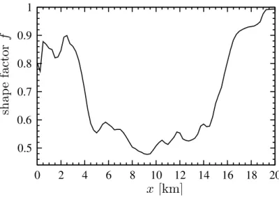
Following the approach of Nye (1965), the relation between the shape factor and the ice thickness in the central flow line is inferred from three-dimensional full-Stokes sim-ulations of an infinitely long glacier flowing over a parabola-type bedrock using di_fferent 5

values of the friction paramter. All these three-dimensional simulations (not shown here), are well reproduced with a two-dimensional flow line model using the following empirical estimate of the shape factor:

f=2 πarctan

0.8146

√

a_·h !

, (4)

where h(x)₌zs(x)−b(x) is the ice thickness. Figure 1 shows the evolution of the 10

shape factorf(x) along the flow line for the 1973 geometry.

The ice rheology is described through a power-type flow law, known as Glen’s law in glaciology, linking the strain-rate tensorε˙ to the deviatoric stress tensorτ such as:

˙

ε=Aτ_en−1τ, (5)

15

whereτe2=τi jτi j/2 is the square of the second invariant of the deviatoric stress andA a rheological parameter, which depends on the ice temperature via an Arhenius law. Since the Variegated Glacier is temperate, the constant value A=100 MPa−3a−1 is adopted (close to the ones proposed in Cu_ffey and Paterson, 2010).

2.2 Boundary conditions

20

The upper surfaceΓs, i.e. z=zs, is a stress-free surface and the following Neumann-type boundary condition applies:

(9)

TCD

5, 1461–1494, 2011

Title Page

Tables Figures

◭ ◮

Back Close

Full Screen / Esc

Discussion

P

a

per

|

Dis

cussion

P

a

per

|

Discussion

P

a

per

|

Discussio

n

P

a

per

|

At the bedrock interfaceΓb, i.e.z=b, zero basal melting is assumed (u·n=0) as well as a linear friction law (Robin type boundary condition). This linear friction law relates the basal dragτ_nt to the sliding velocityu_tsuch as:

τ_nt=t_·(σ_·n)_|_b=−βu_·t=−βu_t forz=b, (7) wheren and t are the normal and tangent unit vectors to the bedrock surface, and 5

β≥0 is the basal friction parameter.

All these equations are solved using the finite element method with the code Elmer/Ice. More details on the numerics can be found in Gagliardini et al. (2007) and Gagliardini and Zwinger (2008).

3 The inverse problem

10

3.1 Robin method

The inverse problem is, for each dataset (surface geometry and velocities), to deter-mine the basal friction parameterβthat gives the smallest mismatch between observed and modelled surface velocities.

We use the inverse Robin method adapted to glaciology by Arthern and Gudmunds-15

son (2010). The method consists in solving alternately the Neumann-type problem defined by Eqs. (1, 2) and the surface boundary conditions (6), and the associated Dirichlet-type problem defined by the same equations excepted that the Neumann upper-surface condition (6) is replaced by a Dirichlet condition, such as:

u(zs)=uobs, (8)

20

(10)

TCD

5, 1461–1494, 2011

Title Page

Tables Figures

◭ ◮

Back Close

Full Screen / Esc

Discussion

P

a

per

|

Dis

cussion

P

a

per

|

Discussion

P

a

per

|

Discussio

n

P

a

per

|

The cost function that expresses the mismatch between the solution of the two mod-els on the upper surface_Γ_sis given by

J_o= Z

Γs

(uN₋uD)_·(σN₋σD)_·nd_Γ, (9)

where superscripts N and D refer to the Neumann and Dirichlet problem solutions, respectively.

5

The G ˆateaux derivative of the cost functionJ_owith respect to the friction parameter

βfor a perturbationβ′is given by (Arthern and Gudmundsson, 2010):

d_βJ_o= Z

Γb

β′_|uD_|2_−|uN_|2dΓ, (10)

where the symbol_|._|defines the norm of the velocity vector.

In this paper, to avoid unphysical negative values of the friction parameter,β is ex-10

pressed as

β=10α. (11)

The optimisation is now done with respect toα and the G ˆateaux derivative ofJ_o with respect toα is obtained as follows:

d_αJ_o=d_βJ_odβ

dα = Z

Γb

β′_|uD_|2_−|uN_|210αln(10)dΓ. (12) 15

In the presence of noise in the observed velocities, the method can lead to spuri-ous small wavelength oscillations of the inferred friction parameter. Arthern and Gud-mundsson (2010) suggest to stop the minimisation when the cost function starts to stagnate at a certain level. Furthermore, the authors show that this is in agreement with a heuristic stopping criterion based on the observation errors. One drawback of 20

(11)

TCD

5, 1461–1494, 2011

Title Page

Tables Figures

◭ ◮

Back Close

Full Screen / Esc

Discussion

P

a

per

|

Dis

cussion

P

a

per

|

Discussion

P

a

per

|

Discussio

n

P

a

per

|

errors could vary strongly from one place to another, but also from one dataset to an-other, so that the stopping criterion should be di_fferent for each area and each dataset. Here, an additional Tikhonov regularisation term that penalises the small wavelength oscillations of the friction parameterβ, taken as

J_reg= Z

Γb

∂α ∂x

!2

dΓ, (13)

5

is added to the cost functionJo. The total cost function now writes

J_tot=J_o+1

2λu¯

obs_J

reg, (14)

where ¯uobs is the mean value of the observed surface velocities andλis a weighting parameter used to adjust the influence of the added regularisation with respect to the initial cost function. The term ¯uobs takes into account the large changes in velocity ob-10

served along the 10-year dataset and allows to use a unique value of theλparameter for all the datasets. Regularisation is classical in data assimilation: the minimisation ofJ_o alone is an ill-posed problem, and the addition of a regularisation term ensures existence of a global minimum. IfΛis large enough, the problem becomes well-posed, with a unique minimum, and therefore the minimisation algorithm shows improved con-15

vergence properties. The form of the additional term ensures that the optimal α is smooth. The effect of this regularisation term and the sensitivity of theβdistribution to the parameterλis discussed in the results Section.

The minimisation of the cost functionJ_tot with respect toβis done using the limited memory quasi-Newton routine M1QN3 (Gilbert and Lemar ´echal, 1989) implemented 20

(12)

TCD

5, 1461–1494, 2011

Title Page

Tables Figures

◭ ◮

Back Close

Full Screen / Esc

Discussion

P

a

per

|

Dis

cussion

P

a

per

|

Discussion

P

a

per

|

Discussio

n

P

a

per

|

3.2 Technical aspects

The Stokes equations and the Robin problem are solved using the finite element code Elmer/Ice. For each date, a regular mesh is constructed using 80 horizontal times 20 vertical layers of quadrangle elements, between the bedrock and upper surface. For non-icy areas, a minimal thickness of 3 m is imposed to avoid zero volume elements. 5

Each of the 25 datasets is composed of the surface elevation and the horizontal sur-face velocity at 81 points regularly spaced every 250 m along the 20 km of the glacier length. Topographic measurements are representative of a given date whereas veloc-ity measurements refer to the period in-between two measurement dates (Raymond and Harrison, 1988). For the quiescent period, the same surface topography is used 10

for the summer and for the following winter. For the surge, because of the fast chang-ing topography, for a given velocity measurement, the surface topography is taken as the median of the two surface topographies corresponding to the surface velocity mea-surement dates. To construct the 25 geometries corresponding to the 25 datasets, the surface elevation must be defined along the whole glacier. Where surface topography 15

measurements are missing, the elevation is estimated from the other datasets using a linear adjustment to fulfil the current surface elevation continuity. For the velocity, the mesh is constructed so that point measurements and mesh nodes coincide. When solving the Dirichlet problem, measured velocities are imposed only where measure-ments are available and no interpolation is used to complete missing data. We verified 20

that a finer mesh does not change significantly the results of the inversion of the friction parameter.

4 Inversion of the basal friction parameter

4.1 Influence of the regularisation term

We used the most complete summer 1978 dataset to assess the influence of the reg-25

(13)

TCD

5, 1461–1494, 2011

Title Page

Tables Figures

◭ ◮

Back Close

Full Screen / Esc

Discussion

P

a

per

|

Dis

cussion

P

a

per

|

Discussion

P

a

per

|

Discussio

n

P

a

per

|

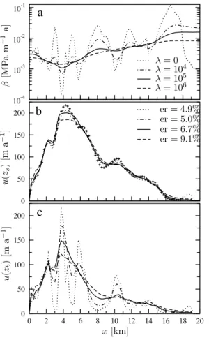
surface and sliding velocities obtained for different values of the regularisation param-eter λ are shown in Fig. 2. For the case with no regularisation, the iterations were stopped after 54 iterations when the cost function started to stagnate. The case where

λ=0 allows the best match with the observed velocities with a relative mean error equal to 4.9 %, but shows large variations of the friction coe_fficient (Fig. 2a) which result in 5

large variations of the sliding velocity (Fig. 2c). The wavelength of the oscillations is larger than the mesh spacing and thus does not correspond to the short wavelength oscillations associated with the error noise presented by Arthern and Gudmundsson (2010).

With a non-zero regularisation term, at the scale of the glacier, the mean value of 10

the inferred friction parameter is very similar for all the values ofλbut the oscillations are smoothed and the smoothing is greater as λincreases. The di_fference between modelled and observed surface velocities remains small, but the short wavelength oscillations of the observed velocities are less well resolved when the regularisation term increases. As a result, the corresponding sliding velocities, illustrated in Fig. 2c, 15

are also smoothed by the regularisation and some points show very large differences compared with no regularisation (λ=0). The comparison between surface and basal velocities shows that all these small wavelength oscillations arising at the base have almost no visible influence at the glacier surface.

The relative mean error increases from 5.0 % to 9.1 % whenλis increased from 104 20

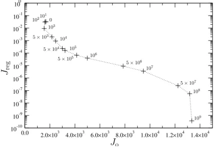
to 106. If in reality high and low friction areas may alternate, other approximations or uncertainties (such as the topography or 3-D effects) may explain the oscillations obtained with no regularisation. A smoothed distribution is thus preferred. Neverthe-less, the optimal regularisation parameterλcan be estimated using a L-curve analysis (Hansen, 2001). The L-curve method uses the plot of the norm of the regularised so-25

lutionJreggiven by Eq. (13) versus the norm of the initial cost functionJo(9) to choose

(14)

TCD

5, 1461–1494, 2011

Title Page

Tables Figures

◭ ◮

Back Close

Full Screen / Esc

Discussion

P

a

per

|

Dis

cussion

P

a

per

|

Discussion

P

a

per

|

Discussio

n

P

a

per

|

by one order on magnitude when λis varied from 0 to 109, which is relatively low in comparison to other applications. Note that the L-curve analysis should be conducted for all dataset and might conduct to di_fferent values of the regularisation parameter de-spite the ponderation by ¯uobs of the regularisation term in (14). Because this analysis necessitate a large number of simulations, it was not reasonably feasible for the 25 5

datasets, and in what follow, the valueλ=105is then adopted for all the datasets.

4.2 Inferred basal friction parameter distributions

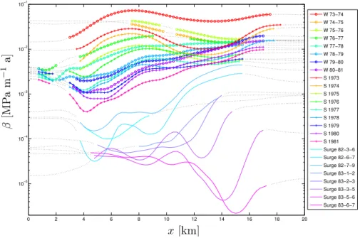
The distribution of the friction parameter was inferred using the same method for the 25 datasets available during the quiescent phase and the surge. Results are shown in Fig. 4. Seasonal changes between summer and winter can be observed. For a given 10

year, the winter always presents higher friction than the previous summer. But, during the eight years of the quiescent phase, the friction parameterβregularly decreases, so that the last winter values are smaller than the first summer ones. Another remarkable feature is that the friction decrease is more pronounced in the upper part of the glacier than in the lower part during the quiescent phase. Contradictory to the assumption 15

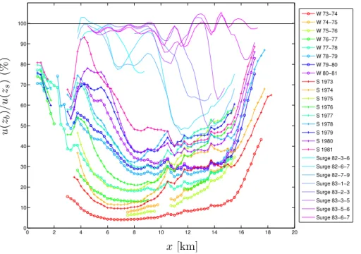
made by Bindschadler (1982), our results indicate that sliding already contributes for a large part of the total motion of the glacier during the quiescent phase. As shown in Fig. 5, the contribution of the basal velocity continuously increases during the quiescent phase, from a mean value of 10 % in winter 1973 up to 60 % for summer 1981 just before the surge started, confirming the values inferred by Raymond and Harrison 20

(1988) using a simple model.

At the onset of the surge in winter 1981–1982, dramatic changes in the basal fric-tion occurre. The inferred fricfric-tion parameter drops by about one order of magnitude from 10−3 to 10−4MPa m−1a, causing a high increase of the basal sliding, as shown in Figs. 4 and 5. After this onset phase, the friction continues to decrease regularly 25

(15)

TCD

5, 1461–1494, 2011

Title Page

Tables Figures

◭ ◮

Back Close

Full Screen / Esc

Discussion

P

a

per

|

Dis

cussion

P

a

per

|

Discussion

P

a

per

|

Discussio

n

P

a

per

|

to September 1982 and ends with a punctual increase of the basal friction. The second phase starts in January 1983 and spreads down the glacier until July 1983 with a dra-matic decrease of the basal friction. During the second part of the surge, we observe the propagation of a low basal friction area from the middle part of the glacier down to its terminus. At the end of the surge, the basal sliding accounts for more than 90 % 5

of the observed surface velocities everywhere on the glacier, whereas it is only the case in the upper part during the first phase of the surge. Fig. 5 shows that in some places along the flow line, basal velocities are greater than the surface ones. This is possible because of the stress transmission when solving the Stokes system with no simplification.

10

The inversion procedure allows gives a good representation of the observed veloc-ities of each date of the 10-year dataset. The observed changes in surface velocveloc-ities during the quiescent and surge phases can be explained by changes in the basal sliding velocity and thus are clearly visible in the inferred distributions of the friction parameter β. Here, the simplest linear friction law (7) is assumed, in which the fric-15

tion parameterβencompasses all the complexity of basal friction. In the next section, following the idea proposed by Flowers et al. (2011), the inferred friction parameter dis-tributionβ(x_i,t_j) (i=1,81 points andj=1,25 dates) is interpreted in terms of changes of the effective pressure at the base of the Variegated Glacier from 1973 to 1983, using a more complex friction law.

20

5 Basal water distributions

5.1 A water-dependent friction law

Many authors have attempted to infer from physical and mathematical considerations which variables should be incorporated in a realistic friction law (e.g., Weertman, 1957; Lliboutry, 1968, 1979; Nye, 1969, 1970; Kamb, 1970, 1987; Morland, 1984; 25

(16)

TCD

5, 1461–1494, 2011

Title Page

Tables Figures

◭ ◮

Back Close

Full Screen / Esc

Discussion

P

a

per

|

Dis

cussion

P

a

per

|

Discussion

P

a

per

|

Discussio

n

P

a

per

|

from mathematical developments, and Gagliardini et al. (2007) from finite element sim-ulations have both proposed a similar friction law for the flow of clean ice over a rigid bedrock in presence of cavitation. In its simplest form, where the basal drag tends asymptotically to its maximum value (post-peak exponent q=1 in Gagliardini et al. (2007)), this friction law is of the form:

5

τ_nt N =C





u(1_t −n) CnNnAs+ut





1/n

ut. (15)

In the above equation, As is the sliding parameter in the absence of cavitation and n Glen’s law exponent, resulting in a non-linear relation between the basal dragτnt and the basal sliding velocityu_t. Note that in the limit case where n=1 and N_≫0, the sliding parameterAsand the friction parameterβare inversely proportional. As shown 10

by Schoof (2005), the coe_fficientC is lower than the maximum local positive slope of the bedrock topography at a decimetre to meter scale, so that the ratioτ_nt/N_≤Cfulfils Iken’s bound (Iken, 1981). The friction law (15) is strongly related to the water pressure

pw through the effective pressureN=−σnn−pw. Whenpw=0, the effective pressure is equal to the normal compressive Cauchy stress, and increasing water pressure leads 15

to a decrease ofN toward zero. The two parametersA_s=A_s(x) andC=C(x) are only a function of space whereas the time-dependent changes are due to changes in the effective pressureN=N(x,t). Note that effective pressure changes reflect changes in water pressure and/or basal normal stress, as discussed below.

AssumingAs andCare known, the effective pressure, and thus the water pressure, 20

can be evaluated from the previous inversion results for all pointsx_i and all datest_j, as follows:

N(x_i,t_j)₌ βut

C1₋βnu_t(n−1)A_s1/n

, (16)

(17)

TCD

5, 1461–1494, 2011

Title Page

Tables Figures

◭ ◮

Back Close

Full Screen / Esc

Discussion

P

a

per

|

Dis

cussion

P

a

per

|

Discussion

P

a

per

|

Discussio

n

P

a

per

|

Physically, the e_ffective pressure is bounded, i.e. 0< τnt/C≤N≤ −σnn, but the eval-uation ofN(x_i,t_j) from (16) can be out of these bounds due to the assumed A_s and

C distributions. The effective pressure being inversely proportional to the coefficient

C >0, we will hereafter assume a uniform C (C=0.5) and discuss the bound issue only in terms ofA_s. The upper boundN_{≤ −}σ_nn(orp_w_≥0) is violated where the sliding 5

parameterA_s is too high, so that even with zero water pressure the sliding velocity is too great. The boundN≥τnt/C(orpw≤ −σnn−τnt/C, remindingσnn<0 andτnt>0) is never violated since it corresponds to infinitely great sliding velocity.

By considering the upper bound it is possible to estimate the sliding parameter in absence of cavitation As so that N≤ −σnn is always fulfilled. Assuming zero water 10

pressure, the distribution of the minimal sliding parameterAmin_s can be evaluated from Eqs. (7 and 15) in whichpw=0, such as:

Amin_s (xi)=min tj

(As(xi,tj))=min tj



 u(1_t −n)

βn − u_t Cn(₋σnn)n



, (17)

where β, σnn and ut are defined at each date tj and each point xi where data are available. It is found that the minimal value of A_s inferred from (17) is everywhere 15

obtained for the winter 1973 dataset, except for the upper and lower points for which no measurements were performed in 1973. This indicates that basal sliding during winter 1973 represents the lowest values in the following 10-year period.

5.2 Modelled change in basal water pressure

Using the inferred sliding parameter distributionAmin_s (x), the water pressure for the 25 20

dates is then obtained from Eq. (16). Figure 6 shows the evolution with time (vertical axis) and space (horizontal axis) of the ratio of the water pressure over the normal stress₋p_w/σ_nn. This ratio is plotted instead of the effective pressureN because it is visually easy to interpret. When this ratio tends toward 1, the effective pressure tends toward zero and the sliding is increased.

(18)

TCD

5, 1461–1494, 2011

Title Page

Tables Figures

◭ ◮

Back Close

Full Screen / Esc

Discussion

P

a

per

|

Dis

cussion

P

a

per

|

Discussion

P

a

per

|

Discussio

n

P

a

per

|

The first noticeable result is that the large changes in the friction parameterβshown in Fig. 4 are induced by relatively small changes in terms of water pressure. In fact, as shown in Fig. 7, the basal normal stress is almost constant during the 10-year period, despite strong variations along the flow line. Therefore, changes with time of the ratio

−pw/σnn are mostly due to changes in water pressure. As shown in Fig. 6, the ratio 5

−p_w/σ_nnonly evolves between 0.7 to 1, if we except the winter 1973 for which it is zero due to the definition of theA_s parameter. This can be explained by the shape of the friction law used and the fact that it is bounded (see Fig. 8 in Gagliardini et al., 2007). For low sliding velocity corresponding to great e_ffective pressure, a great increase in water pressure is needed to increase the velocity. For great sliding velocity, it is the 10

opposite, due to the asymptotical behaviour of the friction law, i.e. a small increase in water pressure leads to great increase in velocity.

Note, that even if the normal stressσ_nn is almost constant, a slight and progressive increase ofσnn in the upper part of the glacier is visible in the years before the surge, induced by an increase of the observed ice thickness. During the surge, this increase 15

propagates down the glacier attesting displacement of the ice mass.

Again, the seasonality of the sliding is visible in Fig. 6, as well as the two phases of the surge. Also, as was already inferred from theβinversion, the geatest changes are observed in the upper part of the glacier during the quiescent phase and the first surge phase. For the second phase of the surge, we observe the propagation of a high water 20

pressure area from the upper part to the lower part of the glacier, while the pressure in the upper part still remains significant. During this last stage, the increase of water pressure, even though relatively small (2–6 %), leads to very large increase of the ice flow.

5.3 Effect of basal topography on basal water pressure

25

(19)

TCD

5, 1461–1494, 2011

Title Page

Tables Figures

◭ ◮

Back Close

Full Screen / Esc

Discussion

P

a

per

|

Dis

cussion

P

a

per

|

Discussion

P

a

per

|

Discussio

n

P

a

per

|

that these are the areas where the increase of the water pressure is the highest. These bedrock bumps, and more particularly the one located atx=10 km, seem to restrain the water in an upstream catchment. This interpretation is consistent with the surge hypothesis formulated by Lingle and Fatland (2003). Indeed, the progressive evolution of the surface topography of Variegated Glacier leads to an increasingly constricted 5

water catchment upstreamx=10 km, which increases slightly the water pressure up to a threshold value for which the surge occurs. During the second phase of the surge, the propagation of the high water pressure area downstreamx=10 km (Fig. 6) is probably a consequence of the destruction of the water catchment during the first surge stage, leading to the opening of the initially constricted water catchment.

10

6 Direct prognostic simulations

From the previous analysis, the friction parameterβis reconstructed for the 25 datasets from summers 1973 to 1983. To test the sensitivity of the model to the surface ge-ometry, from the inferred history of the friction parameter, we run a prognostic time-dependent simulation assuming a constant mass balance over these 10 years.

15

Starting from the summer 1973 surface geometry, the upper free surface is evolved using the following kinematic boundary condition:

∂z_s ∂t +ux

∂z_s

∂x −uz=as, (18)

where as is the accumulation/ablation function. This function is estimated from the average mass balance measured on Variegated Glacier between 1972 to 1976 (Bind-20

schadler, 1982). The mass balance is supposed to be linearly dependent on the sur-face altitudezs and the equilibrium line located at 1050 m.a.s.l., such as:

a_s=min 6zs−1050 885 ;3.2

!

(20)

TCD

5, 1461–1494, 2011

Title Page

Tables Figures

◭ ◮

Back Close

Full Screen / Esc

Discussion

P

a

per

|

Dis

cussion

P

a

per

|

Discussion

P

a

per

|

Discussio

n

P

a

per

|

The Stokes Eqs. (1 and 2) using the basal boundary condition (7), and the free surface evolution Eq. (18) are coupled and solved iteratively using a time step of 0.1 a. At each time step, the basal friction parameterβ is interpolated linearly from the two closest datasets in the time-series.

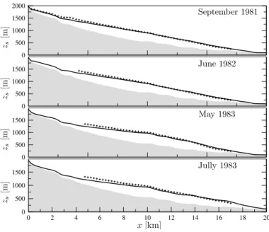
The modelled surface is compared with the observed surface at four di_fferent dates 5

just before, during and after the surge in Fig. 8. The modelled and observed surface elevations before and during the surge relative to the measured surface elevation of summer 1973 are shown in Figs. 9 and 10. Before the surge we observe a thickening of the upper part of the glacier and a thinning of the lower part. The timing and the magnitude of the changes are well reproduced by the model except on the highest 10

part of the glacier where the model leads to a thinning of the glacier. Part of the discrepancies between the model and observations can be explained by errors in the mass balance and/or by three-dimensional effects (ice convergence along the central flow line, Raymond, 1987) as the observed volume increases whereas, in the model, the integrated mass balance is slightly negative leading to a decrease of the modelled 15

ice volume.

The modelled surge occurs in phase with the observations when the friction param-eter dramatically decreases in March 1982. The surge is characterised by a thinning of the upper part of the glacier and a thickening of the lower part which results in the advance of the ice front. As already observed for the quiescent phase, the upper part 20

of the glacier is too thin when compared with summer 1973, but the timing of the mass transfer from the upper part to the lower part of the glacier is well captured by the model, and particularly the advance of the ice front position.

The ability of our model to reproduce the main characteristics of the surge validates a posteriori the use of the diagnostic model to infer the basal friction distribution for each 25

(21)

TCD

5, 1461–1494, 2011

Title Page

Tables Figures

◭ ◮

Back Close

Full Screen / Esc

Discussion

P

a

per

|

Dis

cussion

P

a

per

|

Discussion

P

a

per

|

Discussio

n

P

a

per

|

on the modelled topography can be easily explained by the lack of data (topography, velocities and mass balance) and three-dimensional e_ffects.

7 Conclusions

We have presented the first application to a real case of the inverse method proposed by Arthern and Gudmundsson (2010). It demonstrates the strong relevance of this 5

inverse method, which allowed the reconstruction with a high accuracy of the basal conditions below Variegated Glacier along a 10-year period. From this reconstruction of the friction parameter, the water pressure was inferred using a water pressure de-pendent friction law. As an important result, we showed that very large changes in the basal friction parameter are induced by relatively small changes in basal water 10

pressure. This is mainly due to the asymptotical behaviour of the friction law for great sliding velocity. Our results confirm the presence of a subglacial water storage in the mid-upper part of the glacier as proposed by Lingle and Fatland (2003).

To take this study further, our reconstruction of the basal water pressure over the 10-year period should be used to constrain a hydrological model coupled with an ice flow 15

model, as in Pimentel et al. (2010) and de Fleurian et al. (2011). This would, however, need to be conducted using a three-dimensional modelling approach to overcome the limitations of a flowline hydrological model. This would be the last step to fully relate the surge behaviour of Variegated Glacier to its surface mass balance over the decade 1973–1983.

20

Acknowledgements. This work was supported by both the ADAGe project (ANR-09-SYSC-001) funded by the Agence National de la Recherche (ANR) and the ice2sea project funded by the European Commission’s 7th Framework Programme through grant number 226375 (ice2sea publication 32). Part of the computations presented in this paper were performed at the Ser-vice Commun de Calcul Intensif de l’Observatoire de Grenoble (SCCI). The authors thank 25

(22)

TCD

5, 1461–1494, 2011

Title Page

Tables Figures

◭ ◮

Back Close

Full Screen / Esc

Discussion

P

a

per

|

Dis

cussion

P

a

per

|

Discussion

P

a

per

|

Discussio

n

P

a

per

|

The publication of this article is financed by CNRS-INSU.

References

Arthern, R. and Gudmundsson, G.: Initialization of ice-sheet forecasts viewed as an inverse 5

Robin problem, J. Glaciol., 56, 527–533, 2010. 1462, 1465, 1466, 1469, 1470, 1473, 1480, 1481

Bindschadler, R.: A Numerical Model of Temperate Glacier Flow Applied to the Quiescent Phase of a Surge-Type Glacier, J. Glaciol., 28, 239–265, 1982. 1463, 1474, 1479

Bindschadler, R., Harrison, W. D., Raymond, C. F., and Crosson, R.: Geometry and dynamics 10

of a surge-type glacier, J. Glaciol., 18, 181–194, 1977. 1463, 1464

Cuffey, K. and Paterson, W. S. B.: The physics of glaciers, fourth edition, Pergamon, Oxford, 2010. 1468

de Fleurian, B., Gagliardini, O., Zwinger, T., Le Meur, E., and Durand., G.: A coupled hydro-glaciological model to explain post-j ¨okulhlaups dynamics, J. Geophys. Res., in review, 2011. 15

1481

Eisen, O., Harrison, W. D., and Raymond, C. F.: The surges of Variegated Glacier, Alaska, USA, and their connection to climate and mass balance, J. Glaciol., 47, 351–358, 2001. 1463 Eisen, O., Harrison, W., Raymond, C., Echelmeyer, K., Bender, G., and Gorda, J.: Variegated

Glacier, Alaska, USA: a century of surges, J. Glaciol., 51, 399–406, 2005. 1463, 1465 20

Flowers, G. E., Roux, N., Pimentel, S., and Schoof, C. G.: Present dynamics and future prog-nosis of a slowly surging glacier, The Cryosphere, 5, 299–313, doi:10.5194/tc-5-299-2011, 2011. 1466, 1475

Fowler, A. C.: A theoretical treatment of the sliding of glaciers in the absence of cavitation, Phil. Trans. R. Soc. Lond., 298, 637–685, 1981. 1475

(23)

TCD

5, 1461–1494, 2011

Title Page

Tables Figures

◭ ◮

Back Close

Full Screen / Esc

Discussion

P

a

per

|

Dis

cussion

P

a

per

|

Discussion

P

a

per

|

Discussio

n

P

a

per

|

Fowler, A. C.: A sliding law for glaciers of constant viscosity in the presence of subglacial cavitation, Proc. R. Soc. Lond. A, 407, 147–170, 1986. 1475

Fowler, A. C.: Sliding with cavity formation, J. Glaciol., 33, 255–267, 1987. 1475

Gagliardini, O. and Zwinger, T.: The ISMIP-HOM benchmark experiments performed using the Finite-Element code Elmer, The Cryosphere, 2, 67–76, doi:10.5194/tc-2-67-2008, 2008. 5

1469

Gagliardini, O., Cohen, D., R ˚aback, P., and Zwinger, T.: Finite-element modeling of subglacial cavities and related friction law, J. Geophys. Res., 112, F02027, doi:10.1029/2006JF000576, 2007. 1466, 1469, 1476, 1478

Gilbert, J.-C. and Lemar ´echal, C.: Some numerical experiments with variable-storage quasi-10

Newton algorithms, Mathematical Programming, 45, 407–435, 1989. 1471

Goldberg, D. N. and Sergienko, O. V.: Data assimilation using a hybrid ice flow model, The Cryosphere Discuss., 4, 2201–2231, doi:10.5194/tcd-4-2201-2010, 2010. 1466

Gudmundsson, G. H.: Basal-flow characteristics of a linear medium sliding frictionless over small bedrock undulations, J. Glaciol., 43, 71–79, 1997a. 1475

15

Gudmundsson, G. H.: Basal-flow characteristics of a non-linear flow sliding frictionless over strongly undulating bedrock, J. Glaciol., 43, 80–89, 1997b. 1475

Gudmundsson, G. H. and Raymond, M.: On the limit to resolution and information on basal properties obtainable from surface data on ice streams, The Cryosphere, 2, 167–178, doi:10.5194/tc-2-167-2008, 2008. 1465

20

Hansen, P.: The L-curve and its use in the numerical treatment of inverse problems, Computa-tional inverse problems in electrocardiology, 5, 119–142, 2001. 1473

Harrison, W. and Post, A.: How much do we really know about glacier surging?, Ann. Glaciol., 36, 1–6, 2003. 1464

Harrison, W., Motyka, R., Truffer, M., Eisen, O., Moran, M., Raymond, C., Fahnestock, M., and 25

Nolan, M.: Another surge of Variegated Glacier, Alaska, USA, 2003/04, J. Glaciol., 54(184), 192–194, 2008. 1463

Iken, A.: The effect of the subglacial water pressure on the sliding velocity of a glacier in an idealized numerical model, J. Glaciol., 27, 407–421, 1981. 1476

Kamb, B.: Sliding motion of glaciers: theory and observation, Rev. Geophys. Space Phys., 8, 30

673–728, 1970. 1475

(24)

TCD

5, 1461–1494, 2011

Title Page

Tables Figures

◭ ◮

Back Close

Full Screen / Esc

Discussion

P

a

per

|

Dis

cussion

P

a

per

|

Discussion

P

a

per

|

Discussio

n

P

a

per

|

Kamb, B., Raymond, C. F., Harrison, W. D., Engelhardt, H., Echelmeyer, K. A., Humphrey, N., Brugman, M. M., and Pfeffer, T.: Glacier surge mechanism: 1982–1983 surge of Variegated Glacier, Alaska, Science, 227, 469–479, 1985. 1463, 1464

Lingle, C. and Fatland, D.: Does englacial water storage drive temperate glacier surges?, Ann. Glaciol., 36, 14–20, 2003. 1464, 1479, 1481

5

Lliboutry, L.: General theory of subglacial cavitation and sliding of temperate glaciers, J. Glaciol., 7, 21–58, 1968. 1475

Lliboutry, L.: Local friction laws for glaciers: a critical review and new openings, J. Glaciol., 23, 67–95, 1979. 1475

Morland, L. W.: Glacier sliding down an inclined wavy bed, J. Glaciol., 17, 447–462, 1984. 1475 10

Morlighem, M., Rignot, E., Seroussi, H., Larour, E., Dhia, H., and Aubry, D.: Spatial patterns of basal drag inferred using control methods from a full-Stokes and simpler models for Pine Is-land Glacier, West Antarctica, Geophys. Res. Lett., 37, L14502, doi:10.1029/2006JF000576, 2010. 1465, 1466

Nye, J.: The flow of a glacier in a channel of rectangular, elliptic or parabolic cross-section, J. 15

Glaciol., 5, 661–690, 1965. 1467, 1468

Nye, J. F.: A calculation on the sliding of ice over a wavy surface using a Newtonian viscous approximation, Proc. R. Soc. London, Ser. A, 311, 445–467, 1969. 1475

Nye, J. F.: Glacier sliding without cavitation in a linear viscous approximation, Proc. R. Soc. London, Ser. A, 315, 381–403, 1970. 1475

20

Pimentel, S., Flowers, G., and Schoof, C.: A hydrologically coupled higher-order flow-band model of ice dynamics with a coulomb friction sliding law, J. Geophys. Res., 115, F04023, doi:10.1029/2009JF001621, 2010. 1481

Raymond, C. F.: How Do Glaciers Surge? A Review, J. Geophys. Res., 92, 9121–9134, 1987. 1463, 1480

25

Raymond, C. F. and Harrison, W. D.: Evolution of Variegated Glacier, Alaska, USA, prior to its surge, J. Glaciol., 34, 154–169, 1988. 1463, 1464, 1465, 1468, 1472, 1474

Raymond Pralong, M. and Gudmundsson, G. H.: Bayesian estimation of basal conditions on Rutford Ice Stream, West Antarctica, from surface data, J. Glaciol., 57(202), 315–324, 2011. 1465

30

Schoof, C.: The effect of cavitation on glacier sliding, Proc. R. Soc. A, 461, 609–627, 2005. 1466, 1475, 1476

(25)

TCD

5, 1461–1494, 2011

Title Page

Tables Figures

◭ ◮

Back Close

Full Screen / Esc

Discussion

P

a

per

|

Dis

cussion

P

a

per

|

Discussion

P

a

per

|

Discussio

n

P

a

per

|

0 2 4 6 8 10 12 14 16 18 20 0.5

0.6 0.7 0.8 0.9 1

s

❤

❛

♣

❡

❢

❛

❝

t

♦

r

①❬❦ ♠❪

(26)

TCD

5, 1461–1494, 2011

Title Page

Tables Figures

◭ ◮

Back Close

Full Screen / Esc

Discussion

P

a

per

|

Dis

cussion

P

a

per

|

Discussion

P

a

per

|

Discussio

n

P

a

per

|

10-4 10-3 10-2 10-1

0 50 100 150 200

0 2 4 6 8 10 12 14 16 18 20

0 50 100 150 200

a

b

c

☞

❬

▼

P

❛

♠

✶

❛

❪

✉

✭

③

s

✮

❬

♠

❛

✶

❪

✉

✭

③

❜

✮

❬

♠

❛

✶

❪

①✁❦✂✄

✕❂✵ ✕❂☎✵

✹

✕❂☎✵ ✺

✕❂☎✵ ✻

❡r❂✆✿✾✪ ❡r❂✝✿✵✪ ❡r❂✞✿✼✪ ❡r❂✾✿☎✪

(27)

TCD

5, 1461–1494, 2011

Title Page

Tables Figures

◭ ◮

Back Close

Full Screen / Esc

Discussion

P

a

per

|

Dis

cussion

P

a

per

|

Discussion

P

a

per

|

Discussio

n

P

a

per

|

0.0

2.0_×103 4.0_×103 6.0_×103 8.0_×103 1.0_×104 1.2_×104 1.4_×104 10-10

10-9 10-8 10-7 10-6 10-5 10-4 10-3 10-2 10-1 10

❏

r

❡

❣

♦ ✵

✵

✶✵ ✁ ✶✵

✷

✶✵ ✸

✶✵ ✹

✶✵ ✺

✶✵ ✻

✶✵ ✼

✶✵ ✽

✶✵ ✾ ✂✄✶✵

✸

✂✄✶✵ ✹

✂✄✶✵ ✺

✂✄✶✵ ✻

✂✄✶✵ ✼

(28)

TCD

5, 1461–1494, 2011

Title Page

Tables Figures

◭ ◮

Back Close

Full Screen / Esc

Discussion

P

a

per

|

Dis

cussion

P

a

per

|

Discussion

P

a

per

|

Discussio

n

P

a

per

|

0 2 4 6 8 10 12 14 16 18 20

10−5

10−4

10−3

10−2

10−1

W 73−74 W 74−75 W 75−76 W 76−77 W 77−78 W 78−79 W 79−80 W 80−81 S 1973 S 1974 S 1975 S 1976 S 1977 S 1978 S 1979 S 1980 S 1981 Surge 82−3−6 Surge 82−6−7 Surge 82−7−9 Surge 83−1−2 Surge 83−2−3 Surge 83−3−5 Surge 83−5−6 Surge 83−6−7

☞

❬

▼

P

❛

♠

✶

❛

❪

①✁❦ ✂✄

(29)

TCD

5, 1461–1494, 2011

Title Page

Tables Figures

◭ ◮

Back Close

Full Screen / Esc

Discussion

P

a

per

|

Dis

cussion

P

a

per

|

Discussion

P

a

per

|

Discussio

n

P

a

per

|

0 2 4 6 8 10 12 14 16 18 20

0 10 20 30 40 50 60 70 80 90 100

W 73−74 W 74−75 W 75−76 W 76−77 W 77−78 W 78−79 W 79−80 W 80−81 S 1973 S 1974 S 1975 S 1976 S 1977 S 1978 S 1979 S 1980 S 1981 Surge 82−3−6 Surge 82−6−7 Surge 82−7−9 Surge 83−1−2 Surge 83−2−3 Surge 83−3−5 Surge 83−5−6 Surge 83−6−7

✉

✭

③

❜

✮

❂

✉

✭

③

s

✮

✭

✪

✮

① ❬❦♠ ❪

(30)

TCD

5, 1461–1494, 2011

Title Page

Tables Figures

◭ ◮

Back Close

Full Screen / Esc

Discussion

P

a

per

|

Dis

cussion

P

a

per

|

Discussion

P

a

per

|

Discussio

n

P

a

per

|

0 2 4 6 8 10 12 14 16 18 20

0 1 2 3 4 5 6 7 8 9

0 0.1 0.2 0.3 0.4 0.5 0.6 0.7 0.8 0.9

❚

✐

♠

❡

❬

❛

✶

❪

①✁❦✂ ✄

☎

♣

✇

❂

✛

♥

(31)

TCD

5, 1461–1494, 2011

Title Page

Tables Figures

◭ ◮

Back Close

Full Screen / Esc

Discussion

P

a

per

|

Dis

cussion

P

a

per

|

Discussion

P

a

per

|

Discussio

n

P

a

per

|

1 2 3 4 5 6 7 8 9

0 1 2 3 4 5 6 7 8 9 10 11 12 13 14 15 16 17 18 19 20 −0.4

−0.3 −0.2 −0.1 0

1 1.5 2 2.5 3 3.5 4

❚

✐

♠

❡

❬

❛

✶

❪

①✁❦ ✂✄

❅

❜

☎

❅

✆

✝

✛

♥

✞

▼

P

✟

✠

(32)

TCD

5, 1461–1494, 2011

Title Page

Tables Figures

◭ ◮

Back Close

Full Screen / Esc

Discussion

P

a

per

|

Dis

cussion

P

a

per

|

Discussion

P

a

per

|

Discussio

n

P

a

per

|

0 500 1000 1500 2000

0 500 1000 1500

0 2 4 6 8 10 12 14 16 18 20 0

500 1000 1500

③

s

❬

♠

❪

③

s

❬

♠

❪

③

s

❬

♠

❪

③

s

❬

♠

❪

① ❦✁ ✂

❙ ❡♣ t❡✁❜❡ r✶✾✽✶

❏✉♥❡✶✾✽✷

▼❛②✶✾✽✸

❏✉❧❧②✶✾✽✸

(33)

TCD

5, 1461–1494, 2011

Title Page

Tables Figures

◭ ◮

Back Close

Full Screen / Esc

Discussion

P

a

per

|

Dis

cussion

P

a

per

|

Discussion

P

a

per

|

Discussio

n

P

a

per

|

-40 -20 0 20 40 60

0 2 4 6 8 10 12 14 16 18 20 -40

-20 0 20 40 60

③

s

③

s

✶

✾

✼

✸

❬

♠

❪

③

s

③

s

✶

✾

✼

✸

❬

♠

❪

① ✁❦ ✂✄ ✂ ♦❞ ❡❧❧❡❞

✂❡ ❛☎✉ r ❡❞

✆✝✞✟

✆✝✽✆

✠

❜

Investigating changes in basal conditions of Variegated Glacier prior and during its 1982&ndash;1983 surge

TCD

Investigating changes in basal conditions

of Variegated Glacier prior and during its

1982–1983 surge

TCD

TCD

TCD

TCD

TCD

TCD

TCD

TCD

TCD

TCD

TCD

TCD

TCD

TCD

TCD

TCD

TCD

TCD

TCD

TCD

TCD

TCD

TCD

TCD

TCD

a

b

c

TCD

TCD

TCD

TCD

TCD

TCD

TCD

Investigating changes in basal conditions of Variegated Glacier prior and during its 1982–1983 surge