O
CCUPATIONAL
T
ASKS AND
C
HANGES IN THE
W
AGE
S
TRUCTURE
Sergio Firpo
Nicole M. Fortin
Thomas Lemieux
Maio
de 2011
T
T
e
e
x
x
t
t
o
o
s
s
p
p
a
a
r
r
a
a
D
D
i
i
s
s
c
c
u
u
s
s
s
s
ã
ã
o
o
284
C
C
-
-
M
M
i
i
c
c
r
r
o
o
W
W
o
o
r
r
k
k
i
i
n
n
g
g
P
P
a
a
p
p
e
e
r
r
S
S
e
e
r
r
i
i
e
e
s
s
04
Os artigos dos Textos para Discussão da Escola de Economia de São Paulo da Fundação Getulio
Vargas são de inteira responsabilidade dos autores e não refletem necessariamente a opinião da
FGV-EESP. É permitida a reprodução total ou parcial dos artigos, desde que creditada a fonte.
Escola de Economia de São Paulo da Fundação Getulio Vargas FGV-EESP
Occupational Tasks and Changes in the Wage Structure
By Sergio Firpo, Nicole M. Fortin, and Thomas Lemieux∗
Draft: February 2011
This paper argues that changes in the returns to occupational tasks have contributed to changes in the wage distribution over the last three decades. Using Current Population Survey (CPS) data, we first show that the 1990s polarization of wages is explained by changes in wage setting between and within occupations, which are well captured by tasks measures linked to technological change and offshorability. Using a decomposition based on Firpo, Fortin, and Lemieux (2009), we find that technological change and de-unionization played a central role in the 1980s and 1990s, while offshorability became an important factor from the 1990s onwards. JEL: J3, J5
Keywords: wage inequality, polarization, occupational tasks, off-shoring, RIF-regressions.
∗ Firpo: S˜ao Paulo School of Economics, Funda¸c˜ao Getulio Vargas, [email protected]; Fortin and Lemieux:
Most studies on changes in inequality and the wage structure have focused on explanations
based on changes in the returns to traditional measures of skills like education and experience
(e.g. Katz and Murphy, 1992) or institutions (e.g. DiNardo, Fortin, and Lemieux, 1996).1 Until
recently, little attention had been paid to the potential role of occupations in changes in wage
inequality. This situation has changed over the last five years for several reasons.
First, Autor, Levy, and Murnane (2003), Goos and Manning (2007), and Autor, Katz and
Kearney (2006) have proposed a new explanation for changes in wage inequality based on a
more “nuanced” view of skill-biased technological change. The idea is that the introduction of
computer and information technologies has not simply depressed the relative demand for less
skilled workers, as it was assumed in early studies such as Berman, Bound, and Griliches (1994).
Rather, computer and information technologies have depressed the return to “routine” tasks
that can now be executed by computer technologies. Autor, Katz and Kearney (2006) and Goos
and Manning (2007) argue that this nuanced view of technological change can help account
for the polarization of wages that has been observed since the late 1980s. Under this type of
technological change, it is plausible that moderately skilled workers who used to perform routine
tasks experienced a decline in relative wages during this period. Technological change could thus
explain why wages in the middle of the distribution fell more than wages at the bottom and top
end of the distribution.2
This more nuanced view of technological change puts occupations at the forefront of the
in-equality debate since the task content of work (routine nature of the job, cognitive skills required,
etc.) is typically measured at the occupational level.3 Occupations are, therefore, a key
empir-ical channel through which we can assess how technologempir-ical change affects the wage structure.
An important empirical implication of this more nuanced view of technological change, that we
discuss below, is that changes in the wage structure within and between occupations should be
systematically related to the type of tasks performed in these occupations.
A second reason for looking at the contribution of occupations in changes in the wage structure
is offshoring. Early explanations for the role of international trade in changes in inequality have
1
The role of industrial change due to de-industrialisation and foreign competition was also explored in some of the early studies such as Murphy and Welch (1991), Bound and Johnson (1992), and Freeman (1995).
2
Acemoglu and Autor (2011) develop a formal model to show how this could happen in a model with three skill levels (high, middle, and low).
3
focused on the role of trade in final products that are defined at the industry level. It was later
argued (Feenstra and Hanson, 2003) that trade in intermediate inputs was a more promising
explanation for changes in wage inequality than trade in final goods and services. More recently,
Grossman and Rossi-Hansberg (2008) have proposed a model where offshoring figures as a source
of task supply among other competing sources. For instance, a U.S. multinational can hire
computer programmers (middle skilled) in India to update and debug a software product. This
lowers the relative demand for that particular occupation, computer programmers, in the United
States, which then depresses their wages. The work performed, say overnight, by the offshored
programmers, can enhance the productivity of computer software engineers and developers and
contribute to wage increases at the other end of the skill spectrum. As in the case of technological
change, occupations are the key channel through which offshoring can contribute to changes in
wage inequality. This suggests assessing the role of offshoring in changes in the wage structure by
contrasting the evolution of wages and employment in occupations that are potentially offshorable
(e.g. Blinder (2007) and Jensen and Kletzer (2010)) relative to those that are not offshorable.
Although occupations now feature prominently as a possible channel for recent changes in
wage inequality, the role of occupations in these changes has not been systemically investigated
yet. Some studies do suggest an important role for an occupation-based explanations. Goos and
Manning (2007) show that the composition effect linked to changes in the distribution of
occupa-tions accounts for a substantial part of the increase in inequality in the United Kingdom. Autor,
Katz and Kearney (2008) provide evidence that, consistent with a nuanced view of
technologi-cal change, the share of employment in occupations in the middle of the wage distribution has
declined over time. Acemoglu and Autor (2011) explore this point in more detail and also show
evidence that changes in inter-occupation wage differentials are an important factor in the growth
in the variance of U.S. wages since 1980. While these findings suggest a potentially important
role for occupations, it remains to be seen how much of the total change in the distribution of
wages can precisely be accounted for by occupation-based explanations.
The goal of this paper is to fill this gap by systematically investigating the contribution of
occupations to changes in the distribution of U.S. male wages.4 We do so by first presenting a
conceptual model of the labor market where productive skills are rewarded differently in different
occupations, as in a standard Roy model. We argue that this simple model provides a general
way of capturing changes in the wage structure induced by factors like technological change and
4
offshorability. Using Current Population Survey (CPS) data for the years 1988-90 and 2000-02,
we then show that the level and dispersion of wages across occupations have changed substantially
over the 1990s, and that these changes are linked to the task content of occupations. We measure
the task content of occupations using data from the O*NET, and create five indexes of tasks that
arguably capture the potential effect of technological change and offshorability on occupational
wages. We find that task content measures explain well (at least half of the observed variation)
the changes in both the level and dispersion of wages across occupations. This evidence suggests
that changes in occupational wage setting are a promising way of accounting for the U-shaped
feature of changes in the wage distribution (Autor, Katz, and Kearney, 2006, 2008).
Second, we explicitly quantify the contribution of occupations, as summarized by the task
content of jobs, in overall changes in the distribution of wages over the last three decades.
We do so using a decomposition method based on the recentered influence function regression
approach of Firpo, Fortin, and Lemieux (2009, 2011). This approach enables us to evaluate the
contribution of changes in the returns to occupational tasks compared to other explanations such
as de-unionization and changes in the labor market wide returns to general skills (labor market
experience and education). We find that technological change and de-unionization played a
relatively central role in the 1980s and 1990s, but had little effect in the 2000s. Increasing
returns to education played an important role in all three decades, while offshorability became
an important factor in the 1990s and, especially, in the 2000s.
The paper is organized as follows. In Section I, we present a Roy model where the returns to
a variety of skills can be occupation-specific. This model provides a rationale for looking at the
contribution of changes in the occupational wage structure in overall changes in inequality, and
helps connect the task content of occupations with wage setting in these occupations. Section II
describes the wage data used, introduces the measures of task content computed from the O*NET
data, and explains how they are linked to the concepts of technological change and offshorability.
Section III documents the changes in the level and dispersion of wages across occupations and
shows that they are connected to our measures of the task content of jobs. The second part of
the paper begins, in Section IV, with a short exposition of the decomposition methodology based
on recentered influence function regressions. The ensuing results are presented in Section V and
I. Wage Setting in Occupations
A. Roy Model of Wage Setting
Most of the wage inequality literature follows a traditional Mincerian approach where wages
are solely determined on the basis of (observed and unobserved) skills. Equilibrium skill prices
depend on supply and demand factors that shape the evolution of the wage structure over time.
Underlying changes in demand linked to technological change and offshoring can certainly have an
impact on the allocation of labor across industry and occupations, but ultimately wage changes
are only linked to changes in the pricing of skills. Acemoglu and Autor (2011) refer to this
model as the “canonical model” that has been used in many influential studies such as Katz and
Murphy (1992), for example.
There is increasing evidence, however, that the canonical model does not provide a
satisfac-tory explanation for several important changes in the wage structure observed over the last few
decades. This is discussed in detail in Acemoglu and Autor (2011) who mention, among other
things, two important shortcomings of the canonical model that are particularly important in
the context of this paper. First, the canonical model does not easily account for differential
changes in inequality in different parts of the distribution, such as the “polarization” of the wage
distribution of the 1980s. Second, the model does not provide insight on the contribution of
occupations to changes in the wage structure because it does not draw any distinction between
“skills” and “tasks”. Acemoglu and Autor (2011) address these shortcomings by proposing a
Ricardian model of the labor market that incorporates a clear distinction between skills and
tasks. This model goes a long way towards explaining the recent changes in the wage structure
that are hard to account for using the canonical model.
Relative to Acemoglu and Autor (2011), we go one step further here by allowing wages to
vary across occupations conditional on the skills of workers, as in the standard Roy model. In
Acemoglu and Autor’s Ricardian model, workers with different levels of skills are systematically
allocated to different occupations on the basis of comparative advantage. But, critically, the law
of one price holds within each skill group in the sense that wages are equalized across occupations,
conditional on skill.
Unlike Acemoglu and Autor, we do not develop a full model of the labor market showing how
skills are allocated to occupations (i.e. tasks), and how wages across skills and tasks are set
tasks, follows a long tradition in labor economics. In Welch (1969), the wagewit of worker iat
timetis set as follows:
(1) wit=θt+
K
X
k=1
rktSik+uit,
where the Sik’s (for k = 1, ..., K) are skill components embodied in worker i, and uit is an
idiosyncratic error term. Therkt’s are the returns (or “prices”) to each skill componentk, while
θt is a base payment that a worker receives regardless of her skills.
As first pointed out by Rosen (1983), Welch (1969)’s model where wages solely depend on the
bundle of skills supplied by each worker is unlikely to hold when workers are allocated to different
tasks or occupations. Consider what happens when workers have the choice between several
occupations that have different production functions (or skill requirements). Following Rosen
(1983) and Acemoglu and Autor (2011), assume that the production function in an occupation
simply depends on the sum of skills supplied by all workers in the occupation. Then, for each
skillk, the aggregate supply of skill in the occupation is the sum ofSik over all workers iin the
occupation. Rosen (1983) shows that returns to skill only get equalized across occupations if
there is sufficient heterogeneity in skill mix across workers to accommodate the large differences
in skill requirements across occupations.
To take a simple example, consider two occupations, mathematicians and movers, and two
skills, cognitive and physical strength. Clearly, cognitive skills are a particularly productive
skill for mathematicians, while physical strength is essential for movers. Say, for instance, that
the marginal product of cognitive and physical skills will only be equalized across these two
occupations if the cognitive/physical skill ratio is 10 for mathematicians, and 0.1 for movers.
Because workers move into an occupation with their own bundle of skills, marginal products
will only be equalized if the average ratio of cognitive to physical skills is 100 times larger for
mathematicians than for movers. Although people who choose to be mathematicians certainly
tend to have a high ratio of cognitive to physical skills, it is very unlikely that people are
heterogenous to the point where it is possible to accommodate the skill ratios required in each
occupation. Therefore, there will be an oversupply of physical skills among mathematicians that
will drive the return to physical skills to almost zero in that occupation. Likewise, there will be
zero. As a result, the return to skill will not be equalized across these two occupations.
The key problem here is that each worker comes with a bundle of skills to be used in a single task
or occupation. If skills could be unbundled and efficiently allocated across occupations, returns
to skill would all get equalized across occupations, as in Welch (1969). Heckman and Sheinkman
(1987) test and soundly reject the unbundling hypotheses by showing that wages systematically
differ across sectors even after controlling for observed and unobserved skills. Gibbons et al.
(2005) reach a similar conclusion when looking at both industry or occupation wage differentials.
In other words, there is a wide range of empirical evidence in support of the Roy model of wage
determination and self selection where skills are rewarded differently in different occupations,
which leads to a systematic sorting of workers into these different occupations. Given the strong
theoretical and empirical reasons why wages and returns to skill may not get equalized across
occupations, in this paper we explore the consequences for the overall wage structure of differences
and changes in wage setting across occupations.5
Generalizing equation (1) to the case where returns to skill vary across occupations k (for
k= 1, .., K) yields the following wage setting equation:
(2) wijt=θjt+
K
X
k=1
rjktSik+uijt,
where wijt is now the wage of individual i in occupation j at time t, the rjkt’s are the returns
(or “prices”) to each skill componentkin occupation j, andθjt is a base payment that a worker
receives in occupationj regardless of her skills.
This wage-setting model is general enough to capture the impact of factors such as technological
change or offshoring on wages. For instance, consider the return to manual dexterity. Prior to
the introduction of sophisticated robots or other computer technologies, manual dexterity was
a highly valued skill in some particular occupations (e.g. precision workers) but not in others
(e.g. sales clerk). When routine manual tasks start getting replaced by automated machines or
robots, this depresses the return to manual dexterity in occupations where these returns were
previously high, but not in others where manual dexterity was not a job requirement.
Similarly, returns to social or communication skills are presumably high in occupations where
5
face-to-face meetings with customers are important (e.g. sale managers). In occupations where
face-to-face meetings are not essential (e.g. computer programmers), however, the returns to
these skills have likely declined as firms are now able to offshore a lot of this work. The general
point here is that the impact of technological change and offshoring can be captured in the above
model by changes in the skill pricing parameters rjkt.
B. Empirical test of the occupational wage setting model
Ideally, we would like to estimate the skill pricing parametersrjkt using repeated cross sections
from a large data set containing detailed information on wages, skills, and occupations. We could
then look at the contribution of changes in occupational wage setting to the overall changes in
the wage structure by computing counterfactual distributions based on alternative measures of
rjkt (andθjt). Unfortunately, no such data set exists. As a result, we instead derive some indirect
predictions from our Roy-type wage setting model (2) to look at the contribution of occupational
wage setting in changes in the wage structure.
A first general prediction of the model is that ifrjktchanges differently in different occupations,
this should have an impact on both the between- and within-occupation dimensions of wage
inequality. The simple intuition for this prediction is that if the return to a skill heavily used in
one occupation goes up, the wage gap between that occupation and others will increase
(between-occupation dimension), and so will the wage dispersion within the (between-occupation (within-(between-occupation
dimension). One first test of whether changes in occupation-specific skill prices contribute to
changes in inequality consists, therefore, in seeing whether there are significant differences in the
changes in both the level and dispersion of wages across occupations.
A second prediction is that changes in both the level and dispersion of wages in occupations
should be systematically related to the task content of occupations. For example, in the O*NET
data, discussed in the next section, economists get a high score on the task “analyzing data or
information”. Presumably, having good cognitive skills is quite important for performing these
types of tasks. In the Roy model, we expect the return to cognitive skills to be high among
economists, so that people with high values of these skills sort into that occupation. To the
extent that the introduction of better computers increases the marginal product of cognitive
skills among economists, we expect both the level and the dispersion of wages (gap between
economists with more and less cognitive skills) to increase for economists, or other occupations
To summarize, although wages depend solely on skills and occupation-specific returns to skill
in equation (2), the task content of occupations should be a useful predictor for changes in both
the level and dispersion of wages across occupations. Another advantage of using the task content
of occupations is that it reduces the dimensionality of the estimation problem by summarizing
a large set of occupation dummies using a more limited number of tasks performed in these
occupations.
If the only distributional statistic of interest was the variance, we could compute the
contribu-tion of occupacontribu-tions to the overall variance by simply looking at the mean and variance of wages in
each occupation, and plugging those into the standard analysis-of-variance formula. Looking at
the variance fails to capture, however, the polarization of the wage distribution that has occurred
since the late 1980s. As a result, we need an alternative way of summarizing changes in the wage
distribution for each occupation that is flexible enough to allow for different changes in different
parts of the distribution.
We do so by first estimating linear regression models that relate the changes in wages at
different quantiles q of the wage distribution for each occupation, ∆wjq, to the corresponding
wage quantile in the base period,wqj0:
(3) ∆wqj =aj+bjwjq0+λq+εqj,
whereλqis a percentile-specific error component, which represents a generic change in the return
to unobservable skills of the type considered by Juhn, Murphy, and Pierce (1993), and εqj is an
idiosyncratic error term. As we explain in more detail in the technical appendix, the
occupation-specific intercepts (aj) and slopes (bj) from these regressions are two summary statistics that
can be directly linked to changes in returns to skill requirements in each occupation, ∆rjk.6 In
addition, the intercept depends on changes in occupational wage differentials that are unrelated
to skills, ∆θj. We use these parameters (aj and bj) to characterize the changes in the wage
distribution for each occupation. The interceptsaj capture between-occupation changes in wage
dispersion, while the slopes bj capture within-occupation changes. As in the single index model
of Card and Lemieux (1996),bj >0 indicates an increase in returns to skill, whilebj <0 indicates
the opposite.
In the second step of the analysis, we link the estimated intercepts and slopes (baj andbbj) to
6
More precisely, we show thataj= ∆θj+PKk=1∆rjkSjkandbj≈1/σ2j0[ PK
k=1 rjk0∆rjk
·σ2
kj+ 1/2∆σ
2
uj], whereσ.j
measures of the task content of each occupation. Since technological change and offshoring are
the key explanatory variables used in the second step, the next section discusses in detail how
we construct five summary measures of occupational tasks. For the time being, define these
summary measures of tasks asT Cjh, forh= 1, ..,5.
The second step regressions are
(4) baj =γ0+
5 X
h=1
γjhT Cjh+µj,
and
(5) bbj =δ0+
5 X
h=1
δjhT Cjh+νj.
There is no direct mapping from the task content measuresT Cjh to the return to skill
param-eters,rjk. We expect to see, however, a steeper decline in the relevantrjkt’s in occupations with
traditional task requirements that are more easily replaceable by technology or offshore workers.
For example, for occupations scoring high in terms of the routine aspect of the work performed,
we should observed negative estimates of bothaj andbj. Similarly, for occupations that involve
face-to-face meetings are less likely to be offshored, we should observed positive estimates ofaj
orbj parameters.
II. Data
A. Wage Data
The empirical analysis is based on data for men from the Outgoing Rotation Group (ORG)
Supplements of the Current Population Survey.7 The wage measure used is an hourly wage
measure computed by dividing earnings by hours of work for workers not paid by the hour. For
workers paid by the hour, we use a direct measure of the hourly wage rate. CPS weights are used
throughout the empirical analysis. At the beginning and end of the three decades we analyze,
we pool several years of data together to improve the precision of the estimates. For the first
period being analyzed (1976-78 to 1988-90), we start with data from the May CPS for the years
1976 to 1978.8 For the second, and main period of analysis, we use 1988-90 as the base year and
7
The data files were processed as in Lemieux (2006b) who provides detailed information on the relevant data issues.
8
2000-02 as the end year to make sure we fully capture all the changes that occurred during the
1990s.9 The base year for the final period is 2003-2004, which does not overlap with the end
year of the 1988-90 to 2000-02 period. The reason for this discrepancy is that there was a major
change in the coding of occupations when the 2000 census classification was introduced in 2003.
For the sake of consistency in the coding of occupations, we only look at post-2002 data when
performing the decomposition for recent years. This explains why the final period we consider
goes from 2003-04 to 2009-10.10
Consistent with Autor, Katz and Kearney (2006), Figure 1 shows that 1988-90 to 2000-02
changes in real wages ($1979) at each percentile of the wage distribution follow a U-shaped
curve. In the figure, we also contrast these wage changes with those that occurred before
(1976-78 to 1988-90) and after (2003-04 to 2009-10) the 1990s. The figure illustrates that wage changes
in the top half of the distribution were quite similar during all time periods, though the changes
have been more modest since 2003. Wages at the very top increased much more than wages in
the middle of the distribution, resulting in increased top-end inequality. By contrast, inequality
in the lower half of the distribution increased rapidly during the 1980s, but decreased sharply
after 1988-90 as wages at the bottom grew substantially more than those in the middle of the
distribution. The bottom part of the distribution has remained more or less unchanged since
2003. This is a bit surprising since recessions are typically believed to have a particularly negative
impact at the bottom end of the distribution. More generally, wage changes for 2003-04 to
2009-2010 should be interpreted with caution since macroeconomic circumstances were very different
during these two time periods. By contrast, the overall state of the labor market was more or
less comparable in the other years considered in the analysis.11
B. Occupational Measures of Technological Change and Offshoring Potential
Like many recent papers (Goos and Manning (2007), Goos, Manning and Salomons (2010),
Crin´o (2010)) that study the task content of jobs, and in particular their offshorability, we use
the precise choice of base year for studying changes in inequality during the 1980s should not have much impact on the results.
9
By pooling three years of data at each end of the sample period, we obtain relatively large samples both in 1988-90 (268,497 observations) and 2000-02 (252,397 observations).
10
Note that there was also a major change in the coding of occupations classification when the 1980 census classification was introduced in 1983. The timing is unfortunate as it coincides with the time period when inequality expanded the most dramatically (1980 to 1984). Since changes in occupational classification were not as dramatic as those that happened in the early 2000s, we used a crosswalk to keep a reasonably consistent definition of occupations between 1976-78 and 1988-90.
11
the O*NET data to compute our measures of technological change and offshoring potential.12
Our aim is to produce indexes for all 3-digit occupations available in the CPS, a feat that
neither Jensen and Kletzer (2007) nor Blinder (2007) completed.13 Our construction of an
index of potential offshorability follows the pioneering work of Jensen and Kletzer (2010) [JK
hereinafter] while incorporating some of the criticisms of Blinder (2007). The main concern of
Blinder (2007) is the inability of objective indexes to take into account two important criteria
for non-offshorability: a) that a job needs to be performed at a specific U.S. location, and b)
that the job requires face-to-face personal interactions with consumers. We thus pay particular
attention to the “face-to-face” and “on-site” categories in the construction of our indexes.
In the spirit of Autor, Levy, and Murnane (2003), who used the Dictionary of Occupational
Titles (DOT) to measure the routine vs. non-routine, and cognitive vs. non-cognitive aspects
of occupations, JK use the information available in the O*NET, the successor of the DOT,
to construct their measures. The O*NET content model organizes the job information into a
structured system of six major categories: worker characteristics, worker requirements, experience
requirements, occupational requirements, labor market characteristics, and occupation-specific
information.
Like JK, we focus on the “occupational requirements” of occupations and also add some “work
context” measures to enrich the “generalized work activities” measures. JK consider eleven
measures of “generalized work activities”, subdivided into five categories: 1) on information
content: getting information, processing information, analyzing data or information,
document-ing/recording information; 2) on internet-enabled: interacting with computers; 3) on face-to-face
contact: assisting or caring for others, performing or working directly with the public,
estab-lishing or maintaining interpersonal relationships; 4) on the routine or creative nature of work:
making decisions and solving problems, thinking creatively; 5) on the “on-site” nature of work:
inspecting equipment, structures or material.
We consider five similar categories, “information content” and “automation”, thought to
be positively related to offshorability (and technology), and “face-to-face”, “on-site job”, and
“decision-making”, thought to be negatively related to offshorability.14 Our first category
“infor-12
Available from National Center for O*NET Development. We use the O*NET 13.0 which has many updated elements by comparison with the O*NET 10.0 used in Goos, Manning and Salomons (2010). Alternatively, using the German IAB/BIBB survey, Spitz-Oener (2006) and Dustmann, Ludsteck and Sch¨onberg (2009) use task measures collected at the worker level.
13
Blinder (2010) did not compute his index for Category IV occupations (533 occupations out of 817), that are deemed impossible to offshore. Although, Jensen and Kletzer (2010) report their index for 457 occupations, it is not available for many blue-collar occupations (occupations SOC 439199 and up).
14
mation content” regroups JK categories 1) and 2). It identifies occupations with high information
content that are likely to be affected by ICT technologies; they are also likely to be offshored if
there are no mitigating factor. Our second category “automation/routinization” is constructed
using some work context measures to reflect the degree of potential automation of jobs and is
an update on the manual routine index of Autor et al. (2003). The work context elements are:
“degree of automation”, “importance of repeating same tasks”, “structured versus unstructured
work (reverse)”, “pace determined by speed of equipment”, and “spend time making repetitive
motions”. We think of these first two categories as being more closely linked to technological
change, thus we called the group “Technology”. We agree with Blinder (2007) that there is some
degree of overlap with offshorability. Indeed, the information content is a substantial component
of JK’s offshorability index.
Our three remaining categories “face-to-face contact”, “on-site job” and “decision-making” are
meant to capture features of jobs that cannot be offshored. Note, however, that the
decision-making features were also used by Autor et al. (2003) to capture the notion of non-routine
cognitive tasks. Our “face-to-face contact” measure adds one work activity “coaching and
devel-oping others” and one work context “face-to-face discussions” element to JK’s face-to-face index.
Our “on-site job” measure adds four other elements of the JK measure: “handling and
mov-ing objects”, “controllmov-ing machines and processes”, “operatmov-ing vehicles, mechanized devices, or
equipment”, and “repairing and maintaining mechanical equipment” and “electronic equipment”
(weight of 0.5 to each of these last two elements). Our “decision-making” measure adds one work
activity “developing objectives and strategies” and two work context elements, “responsibility
for outcomes and results” and “frequency of decision making” to the JK measure. We use the
reverse of these measures of non-offshorability to capture “Offshorability”.
For each occupation, the O*NET provides information on the “importance” and “level” of
required work activity and on the frequency of five categorical levels of work context.15 We follow
Blinder (2007) in arbitrarily assigning a Cobb-Douglas weight of two thirds to “importance” and
one third to “level” in using a weighed sum for work activities. For work contexts, we simply
multiply the frequency by the value of the level. Each compositeT Ch score for occupation j in
15
categoryh is, thus, computed as
(6) T Cjh=
Ah
X
k=1
Ijk2/3L1jk/3+
Ch
X
l=1
Fjl∗Vjl,
whereAh is the number of work activity elements, andCh the number of work context elements
in the categoryT Ch,h= 1, . . .,5.
To summarize, we compute five different measures of task content using the O*NET: i) the
information content of jobs, ii) the degree of automation of the job and whether it represents
routine tasks, iii) the importance of face-to-face contact, iv) the need for on-site work, and v)
the importance of decision making on the job. We use these measures to assess both the impact
of technological change and offshorability on changes in wages.
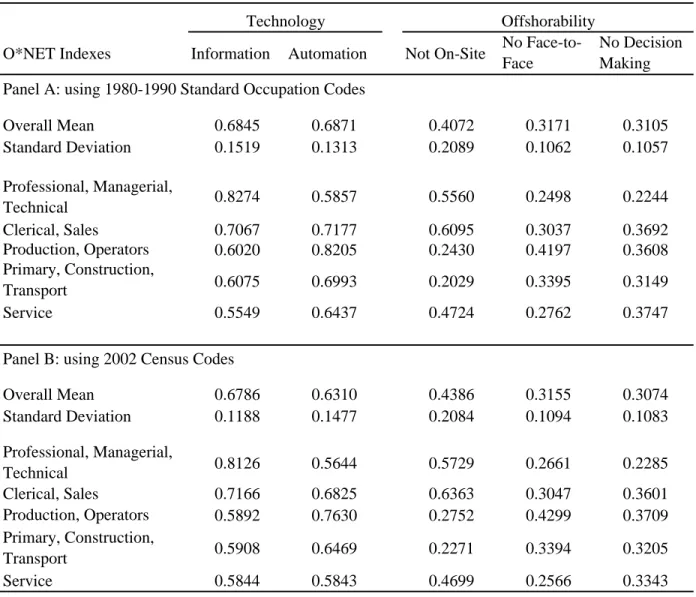
Table 1 shows a number of summary statistics for the five normalized measures of task
con-tent.16 The table reports the average value of the measures of task content for five major
occupational groups. In Panel A, these broad occupations are constructed using the 1980-1990
Census occupation codes. Corresponding measures based on the 2002 census occupation codes
are reported in Panel B. Since most of the empirical analysis presented below focuses on the
1990s, we limit our discussion to the results reported in Panel A.
The results reported in Table 1 are generally consistent with the evidence reported in related
studies. Professional, managerial and technical occupations have the highest score in terms of
their use of information technology, and the lowest score for automation. As a result, these
high wage occupations are likely to benefit the most from technological change. Interestingly,
this broad occupation group also gets the highest score in terms of face-to-face interactions and
decision making, suggesting that they should not be too adversely affected by offshoring.17 At the
other end of the spectrum, production workers and operators have a relatively low score in terms
of their use of information technology and a high score for automation. These jobs also involve
little face-to-face interactions or decision making. Therefore, both offshoring and technological
change are expected to have an adverse impact on wages in these occupations.
The pattern of results for on-site work is more complex. Consistent with our expectations,
primary, construction and transport workers have the highest score for on-site work, while clerical
16
The range of these measures goes from zero to one since we normalize the task measures by dividing them by their maximum value observed over all occupation. These normalized tasks measures provide a useful ranking of occupations along each of these five dimensions, but the absolute values of the task measures have no particular meaning.
17
and sales workers have the lowest score. Interestingly, production workers and operators also get
a high score for working on-site, suggesting that they should not be too affected by offshoring.
This illustrates the limits of the O*NET measures as a way of capturing the offshorability of jobs.
While it is true that production workers tend to work on a specific site, the whole production
process could still be offshored. This is quite different from the case of construction workers for
whom the “site” has to be in the United States. As a result, the effect of on-site work on wages
should be interpreted with some caution.
III. Occupational Wage Profiles: Results
In this section, we first estimate the linear regression models for within-occupation quantiles
from equation (3), and then link the estimated slope and intercept parameters to our measures of
task content from the O*NET as in equations (4) and (5). We refer to these regression models as
“occupation wage profiles”. We focus this first part of the analysis on the 1990s as it represents
the time period when most of the polarization of wages documented by Autor, Katz and Kearney
(2006) occurred.
Note that, despite our large samples based on three years of pooled data, we are left with a small
number of observations in many occupations when we work at the three-digit occupation level. In
the analysis presented in this section, we thus focus on occupations classified at the two-digit level
(40 occupations) to have a large enough number of observations in each occupation.18 This is
particularly important given our empirical approach where we run regressions of change in wages
on the base-period wage. Sampling error in wages generates a spurious negative relationship
between base-level wages and wage changes that can be quite large when wage percentiles are
imprecisely estimated.19 In principle, we could use a large number of wage percentiles, wqjt, in
the empirical analysis. But since wage percentiles are strongly correlated for small differences
in q, we only extract the nine deciles of the within-occupation wage distribution, i.e. wjtq for
q= 10,20, ...,90. Finally, all the regression estimates are weighted by the number of observations
(weighted using the earnings weight from the CPS) in each occupation.
Detailed estimates of several specifications for equation (3) are presented in Appendix Table
18
Though there is a total of 45 occupations at the two-digit level, we combine five occupations with few observations to similar but larger occupations. Specifically, occupation 43 (farm operators and managers) and 45 (forestry and fishing occupations) are combined with occupation 44 (farm workers and related occupations). Another small occupation (20, sales related occupations) is combined with a larger one (19, sales workers, retail and personal services). Finally two occupations in which very few men work (23, secretaries, stenographers, and typists, and 27, private household service occupations) are combined with two other larger occupations (26, other administrative support, including clerical, and 32, personal services, respectively).
19
A3 and discussed in the Technical Appendix. The main finding is that occupation-specific slopes
and intercepts both have to be included in the regression models to adequately account for the
observed wage changes. This general model explains over 90 percent of the variation in the data,
and all of the curvature (or U-shape feature) that characterizes wage changes over that period.
We illustrate the fit of the model by plotting occupation-specific regressions for the 30 largest
occupations curves in Figure 2.20 While it is not possible to see what happens for each and every
occupation on this graph, there is still a noticeable pattern in the data. The slope for occupations
at the bottom end of the distribution tends to be negative. Slopes get flatter in the middle of
the distribution, and generally turn positive at the top end of the distribution. In other words, it
is clear from the figure that the set of occupational wage profiles generally follow the U-shaped
pattern observed in the raw data. In light of the discussion in Section 2, this suggests that skills
that used to be valuable in low-wage occupations are less valuable than they used to be, while
the opposite is happening in high-wage occupations.
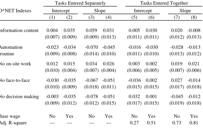
We next explore this hypothesis more formally by estimating the regression models in equations
(4) and (5) that link the intercept and slopes of the occupation wage change profiles to the task
content of occupations.21 The results are reported in Table 2. In the first four columns of Table
2, we include task measures separately in the regressions (one regression for each task measure).
To adjust for the possible confounding effect of overall changes in the return to skill, we also
report estimates that control for the base (median) wage level in the occupation.
As some tasks involving the processing of information may be enhanced by ICT technologies,
we would expect a positive relationship between our “information content” task measure and
the measures of occupational wage changes. On the other hand, to the extent that technological
change allows firms to replace workers performing these types of tasks with computer driven
technologies, we would expect both the intercept and slope of occupational wage changes with
high degree of “automation” to decline over time.22 Although occupations in the middle of the
wage distribution may be most vulnerable to technological change, some also involve relatively
more “on-site” work (e.g. repairmen) and may, therefore, be less vulnerable to offshoring. We
also expect workers in occupations with a high level of “face-to-face” contact, as well as those
20
To avoid overloading the graph, we exclude ten occupations that account for the smallest share of the workforce (less than one percent of workers in each of these occupations).
21
To be consistent with equation (A-8), we have recentered the observed wage changes so that the intercept for each occupation corresponds to the predicted change in wage at the median value of the base wage.
22
with a high level of “decision-making”, to do relatively well in the presence of offshoring.
The strongest and most robust result in Table 2 is that occupations with high level of
automa-tion experience a relative decline in both the intercept and the slope of their occupaautoma-tional wage
profiles. The effect is statistically significant in six of the eight specifications reported in Table
2. The other “technology” variable, information content, has generally a positive and significant
effect on both the intercept and the slope, as expected, when included by itself in columns 1 to
4. The effect tends to be weaker, however, in models where other tasks are also controlled for.
The effect of the tasks related to the offshorability of jobs are reported in the last three rows of
the table. Note that since “on-site”, “face-to-face”, and “decision making” are negatively related
to the offshorability of jobs, we use the reverse of these tasks in the regression to interpret
the coefficients as the impact of offshorability (as opposed to non-offshorability). As a result,
we expect the effect of these adjusted tasks to be negative at the bottom end of the wage
distribution. For instance, the returns to skill in jobs that do not require face-to-face contacts
will likely decrease since it is now possible to offshore these types of jobs to another country.
As discussed earlier and argued by Crisculo and Garicano (2010), increasing the offshoring of
complementary tasks may increase wages at the top end of the wage distribution.
The results reported in Table 2 generally conform to expectations. The effect of “no face to
face” and “no decision making” is generally negative. By contrast, the effect of “no on-site work”
is generally positive, which may indicate that on average we are capturing the positive effect of
offshoring. Another possible explanation is that the O*NET is not well suited for distinguishing
whether a worker has to work on “any site” (i.e. an assembly line worker), vs. working on a site
in the United States (i.e. a construction worker).
More importantly, Table 2 shows that the task measures explain most of the variation in the
slopes, though less of the variation in the intercepts. This suggests that we can capture most of
the effect of occupations on the wage structure using only a handful of task measures, instead of a
large number of occupation dummies. The twin advantage of tasks over occupations is that they
are a more parsimonious way of summarizing the data, and are more economically interpretable
than occupation dummies.23
We draw two main conclusions from Table 3. First, as predicted by the linear skill pricing
model of Section 2, the measures of task content of jobs tend to have a similar impact on the
intercept and on the slope of the occupational wage profiles. Second, tasks account for a large
23
fraction of the variation in the slopes and intercepts over occupations, and the estimated effect
of tasks are generally consistent with our theoretical expectations. Taken together, this suggests
that occupational characteristics as measured by these five task measures can play a substantial
role in explaining the U-shaped feature of the raw data illustrated in Figure 1. These results also
show why models that do no account for within-occupation changes are likely to miss a significant
part of the contribution of the task content of jobs to changes in the wage distribution.
Although the analysis presented above helps illustrate the mechanisms through which
occu-pations play a role in changes in the wage structure, it does not precisely quantify the relative
contribution of occupational factors to these changes.24 We next examine the explanatory power
of occupational tasks in the context of a formal decomposition of changes in the wage distribution.
IV. Decomposing Changes in Distributions Using RIF-Regressions
In this section, we show how to formally decompose changes in the distribution of wages into
the contribution of occupational and other factors using the recentered influence function (RIF)
regression approach introduced by Firpo, Fortin, and Lemieux (2009).25 As is well known, a
standard regression can be used to perform a Oaxaca-Blinder decomposition for the mean of
a distribution. RIF-regressions allow us to perform the same kind of decomposition for any
distributional parameter, including percentiles.
In general, any distributional parameter can be written as a functionalν(FY) of the cumulative
distribution of wages,FY(Y).26 Examples include wage percentiles, the variance of log wage, the
Gini coefficient, etc. The first part of the decomposition consists of dividing the overall change
in a given distributional parameter into a composition effect linked to changes in the distribution
of the covariates, X, and a wage structure effect that reflects how the conditional distribution
of wage F(Y|X) changes over time. In a standard Oaxaca-Blinder decomposition, the wage
structure effect only depends on changes in the conditional mean of wages, E(Y|X). More
generally, however, the wage structure effect depends on the whole conditional wage distribution.
It is helpful to discuss the decomposition problem using the potential outcomes framework.
We focus on differences in the wage distributions for two time periods, 1 and 0. For a worker i,
24
Two limitations of the approach are the linearity of the specification and the focus on the occupation-specific distribution of wages. Also the approach does generally control for other commonly considered factors, such as education, experience, unionization, etc.
25
Firpo, Fortin, and Lemieux (2007, 2011) explain in more detail how to perform these decompositions, and show how to compute the standard errors for each element of the distribution. Here, we simply present a short summary of the methodology.
26
letY1i be the wage that would be paid in period 1, andY0i the wage that would be paid in period
0. Therefore, for eachiwe can define the observed wage,Yi, asYi=Y1i·Ti+Y0i·(1−Ti), where
Ti= 1 if individualiis observed in period 1, andTi= 0 if individual iis observed in period 0.27
There is also a vector of covariatesX ∈ X ⊂RK observed in both periods.
Consider ∆ν
O, the overall change over time in the distributional statisticν. We have
∆νO = ν FY1|T=1
−ν FY0|T=0
=
ν FY1|T=1
−ν FY0|T=1
| {z }
∆ν
S
+
ν FY0|T=1
−ν FY0|T=0
| {z }
∆ν
X
,
where ∆νSis the wage structure effect, while ∆νX is the composition effect. Key to this
decomposi-tion is the counterfactual distribudecomposi-tional statisticsν FY0|T=1
. This represents the distributional
statistic that would have prevailed if workers observed in the end period (T = 1) had been paid
under the wage structure of period 0.
Estimating this type of counterfactual distribution is a well known problem. For instance,
DiNardo, Fortin and Lemieux (1996) suggest estimating this counterfactual by reweighting the
period 0 data to have the same distribution of covariates as in period 1. We follow the same
ap-proach here, since Firpo, Fortin and Lemieux (2007) show that reweighting provides a consistent
nonparametric estimate of the counterfactual distribution under the ignorability assumption.
However, the main goal of this paper is to separate the contribution of different subsets of
covariates to ∆νO, ∆νS, and ∆νX. This is easily done in the case of the mean where each component
of the above decomposition can be written in terms of the regression coefficients and the mean of
the covariates. For distributional statistics besides the mean, Firpo, Fortin, and Lemieux (2009)
suggest estimating a similar regression where the usual outcome variable,Y, is replaced by the
recentered influence function RIF(y;ν) of the statistic ν. The recentering consists of adding
back the distributional statistic ν to the influence function IF(y;ν): RIF(y;ν) = ν + IF(y;ν).
Note that in the case of the mean where the influence function is IF(y;µ) = y−µ, we have
RIF(y;µ) = µ+ (y−µ) = y. Since the RIF(y;µ) is simply the outcome variable y, the
RIF-regression for the mean corresponds to a standard wage RIF-regression.
It is also possible to compute the influence function for many other distributional statistics.
Of particular interest is the case of quantiles. Theτ-th quantile of the distributionF is defined
27
as the functional,Q(F, τ) = inf{y|F(y)≥τ}, or asqτ for short. Its influence function is:
IF(y;qτ) =
τ−1I{y≤qτ} fY (qτ)
.
The recentered influence function of theτth quantile is RIF(y;qτ) = qτ+ IF(y;qτ).
Considerγνt, the estimated coefficients from a regression of RIF(yt;ν) on X
γνt = (E[X·X⊺ |T =t])−1·
E[RIF(yt;νt)·X |T =t], t= 0,1.
Because of the law of iterated expectations, distributional statistics can be expressed in terms of
expectations of the conditional recentered influence functions,
ν(Ft) =EX[E[RIF(yt;ν)|X =x]] =E[X|T =t]·γνt.
In particular, theτthquantile RIF-regression aggregates to the unconditional quantile of interest
and allows us to capture both the between and the within effects of the explanatory variables.
By analogy with the Oaxaca-Blinder decomposition, we could write the wage structure and
composition effects as:
∆νS=E[X|T = 1]⊺
(γν1−γν0) and ∆νX = (E[X|T = 1]−E[X|T = 0])⊺γν
0.
This particular decomposition is very easy to compute since it is similar to a standard
Oaxaca-Blinder decomposition. Firpo, Fortin and Lemieux (2007) point out, however, that there may
be a bias in the decomposition because the linear specification used in the regression is only a
local approximation that does not generally hold for larger changes in the covariates. A related
point was made by Barsky et al. (2002) in the context of the Oaxaca decomposition for the
mean. Barsky et al. point out that when the true conditional expectation is not linear, the
decomposition based on a linear regression is biased. They suggest using a reweighting procedure
instead, though this is not fully applicable here since we also want to estimate the contribution
of each individual covariate.
Firpo, Fortin and Lemieux (2007, 2011) suggest a solution to this problem based on an hybrid
approach that involves both reweighting and RIF-regressions. The idea is that since a regression
when the distribution ofX changes even if the wage structure remains the same. For example,
if the true relationship betweenY and a singleX is convex, the linear regression coefficient will
increase when we shift the distribution ofX up, even if the true (convex) wage structure remains
unchanged. This means that γν
1 and γν0 may be different just because they are estimated for
different distributions ofX even if the wage structure remains unchanged over time.
But reweighting will adjust for this problem. Letting Ψ(X) be the reweighing function,
Ψ(X) = Pr(T = 1|X)/Pr(T = 1)
Pr(T = 0|X)/Pr(T = 0).
that makes the distributions of X’s in period 0 similar to that of period 1, one can estimate the
counterfactual mean asX01=Pi∈0Ψ(b Xi)·Xi−→X1, and the counterfactual coefficientsbγν01as
the coefficients from a regression of RIF(d Y0;ν) on the reweighted sample {X0;Ψ(b X0)}.28 Then
the differencebγν1−bγν01reflects a true change in the wage structure.
The composition effect∆bνX,Rcan be divided into a pure composition effect∆bνX,pusing the wage
structure of period 0 and a component measuring the specification error,∆bνX,e:
b
∆νX,R= X01−X0
b
γν0+X01[bγν01−bγν0].
= ∆bνX,p + ∆bνX,e
(7)
Similarly, the wage structure effect can be written as
b
∆νS,R=X1(bγν1−γbν01) + X1−X01γbν01
= ∆bνS,p + ∆bνS,e
(8)
and reduces to the first term∆bνS,p given that the reweighting error∆bνS,e goes to zero as X01−→
X1.
Again, this decomposition is very easy to compute as it corresponds to two standard
Oaxaca-Blinder decompositions performed on the estimated recentered influence functions. The first
compares time period 0 and the reweighted time period 0 that mimics time period 1 and allows
us to obtain the pure composition effects. The second compares the time period 1 and the
28
reweighted time period 0, and allows use to obtain the pure wage structure effects.
V. Decomposition Results: Occupational Characteristics vs. Other Factors
The covariates included in the regressions reflects the different explanations that have been
suggested for the changes in the wage distribution over our sample period. The key set of
covariates on which we focus are education (six education groups), potential experience (nine
groups), union coverage, and the five measures of occupational task requirements introduced
below. We also include controls for marital status and race in all the estimated models.29
Before showing the decomposition results, it is useful to discuss some features of the estimated
RIF-coefficients across the different wage quantiles.30 For example, the effect of the union status
across the different quantiles is highly non-monotonic. In both 1988-90 and 2000-2002, the
effect first increases up to 0.4 around the median, and then declines (Appendix Figure A2).
This indicates that unions increase inequality in the lower end of the distribution, but decrease
inequality even more in the higher end of the distribution. The results for unions illustrate
an important feature of RIF-regressions for quantiles, namely that they capture the effect of
covariates on both the and within-group components of wage dispersion. The
between-group effect dominates at the bottom end of the distribution, which explains why unions tend to
increase inequality in that part of the distribution. The opposite happens, however, in the upper
end of the wage distribution where the within-group effect dominates the between-group effect.
As in the case of unions, we find that three of our five task measures have non-monotonic impact
across the different percentiles of the wage distribution. Both “information” and “no face-to-face”
have an inverse U-shaped impact, while “automation” has a largely negative U-shaped impact.
Furthermore, changes over time in the effect of these first two task measures shows a declining
effect in the lower middle of the distribution, but an increasing effect in the upper middle of
the distribution. Changes over time in the wage effect of “automation” indicate a large negative
impact in the middle of the wage distribution, with a much smaller impact at the two ends of the
distribution. This is consistent with Autor, Levy and Murnane (2003) who show that workers
in the middle of the distribution are more likely to experience negative wage changes as the
“routine” tasks they used to perform can now be executed by computer technologies. Changes
29
The sample means for all these variables are provided in Appendix Table A1.
30
The RIF-regression coefficients for the 10th, 50th, and 90thquantiles in 1988-90 and 2000-02, along with their (robust)
standard errors are reported in Appendix Table A4. The RIF-regression coefficients for the variance and the Gini are reported in Appendix Table A5. We also plot in Appendix Figure A2 (standard covariates) and Appendix Figure A3 (five task measures) the estimated coefficients from RIF-regressions for 19 different wage quantiles (from the 5th to the 95th
over time in the impact of the other tasks measures appear less important.
The results of the decomposition are presented in Figures 3-5. Tables 3 and 4 also summarize
the results for the standard measures of top-end (90-50 gap) and low-end (50-10) wage inequality,
as well as for the variance of log wages and the Gini coefficient. Note that the base group used in
the RIF-regression models consists of non-union, white, and married men with some college, 15
to 19 years of potential experience, and occupational task measures at half a standard deviation
below their sample averages.31 A richer specification with additional interaction terms is used to
estimate the logit models used in the computation of the reweighting factor.32 The reweighting
approach performs well in the sense that the reweighted means of the covariates for the base
period are very close to those for the end period.33
As is well known (e.g. Oaxaca and Ransom, 1999), the detailed wage structure part of the
decomposition (equation (8)) depends arbitrarily on the choice of the base group. This problem
has mostly been discussed in the case of categorical variables, but it also applies in the case of
continuous variables such as our task content measures.34 Here, we normalize the task measure
variables such that the average difference between the end and beginning period is equal to half
a standard deviation of the raw measure. The wage structure effect for each task measure can be
interpreted as the change over time in the wage impact of a half a standard deviation increase in
the measure.35 We also note that any “composition” effect associated with the task measures are
linked to changes in the shares of occupations over time, as our measures of task requirements
for each occupation are invariant over time.
31
We use “some college” as the base group as it represents the modal education group in the 1990s and 2000s. For the 1976-78 to 1988-90 period, we use high schol graduates as the base group as it was still the modal education group during that period.
32
The logit specification also includes a full set of interaction between experience and education, union status and educa-tion, union status and experience, and education and occupation task measures.
33
The reweighting error is the second term in equation (8). If the reweighting was replicating the means perfectly, we would haveX1 =X01 and the reweighting error would be equal to zero. In Appendix Figure A5, the reweighting error corresponds to the difference between the total composition effect obtained by reweighing and with the RIF-regressions and is found to be very small and not significant.
34
As discussed in Fortin, Lemieux and Firpo (2011), automatic normalization solutions to this issue are not satisfactory, rather the choice of a reasonable and interpretable base group is preferred.
35
A. Overall Decomposition Results
Figure 3 shows the overall change in (real log) wages at each percentileτ, (∆τO), and decomposes
this overall change into a composition (∆τX) and wage structure (∆τS) effect.36 Consistent with
Autor, Katz and Kearney (2006), Figure 3b shows that the overall change between 1988-90 and
2000-02 is U-shaped as wage dispersion increases in the top end but declines in the lower end
of the distribution. This stands in sharp contrast with the situation that prevailed in the early
1980s. Figure 3a shows that the corresponding curve is positively sloped for all quantiles as wage
dispersion increases at all points of the distribution (as in Juhn, Murphy, and Pierce, 1993).
Figure 3c shows that although the wage distribution has been much more stable in recent years,
there is still a modest increase in inequality during the 2003-04 to 2009-10 period. On the one
hand, this is not surprising since the period under consideration is half as long as the two other
periods considered in Figure 3. On the other hand, one could have expected a more dramatic
drop in wages at the bottom end of the distribution given the adverse macroeconomic conditions
of the last few years.
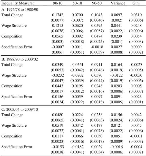
Table 3 summarizes the changes reported in Figure 3 using a few standard measures of wage
dispersion. There is a large increase in inequality measures, such as the variance and the 90-10
gap, that capture wage changes over the entire distribution in the 1980s, and a more modest
increase in later periods. Consistent with Figure 3, inequality at the top end of the distribution
(the 90-50 gap) increases in all time periods. By contrast, the 50-10 gap increases before 1990
and after 2003, but declines substantially during the 1990s.
Figure 3 and Table 3 also show that, consistent with Lemieux (2006b), composition effects have
contributed to a substantial increase in inequality since the late 1970s. For instance, composition
effects account for between 20 percent and 45 percent of the growth in the 90-50 gap in each of
the three time periods. Looking at cumulative changes over all time periods, composition effects
account for all of the change in the 50-10 gap, and about a third of the change in the 90-50 gap.37
But while composition effects account for a sizable part of the growth in overall inequality, it fails
to explain the U-shape pattern observed during the 1990s. As a result, all of the 1990s U-shape
feature in the change in the wage distribution is captured by the wage structure effect.
36
The composition effect reported in Figure 3 only captures the component,∆bν
X,p from equation (8). The specification
error,∆bν
X,e, corresponds to the difference between the total composition effect obtained by reweighting and RIF-regression
methods illustrated in Appendix Figure A4. The figure shows that RIF-regressions capture quite accurately the overall trend in composition effects, though there are a number of small discrepancies at various points along the wage distribution, likely reflecting spikes in the wage distribution.
37
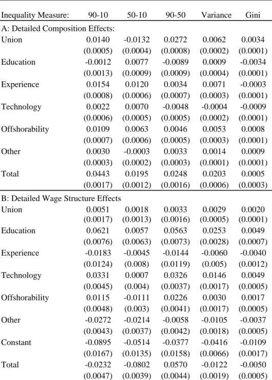
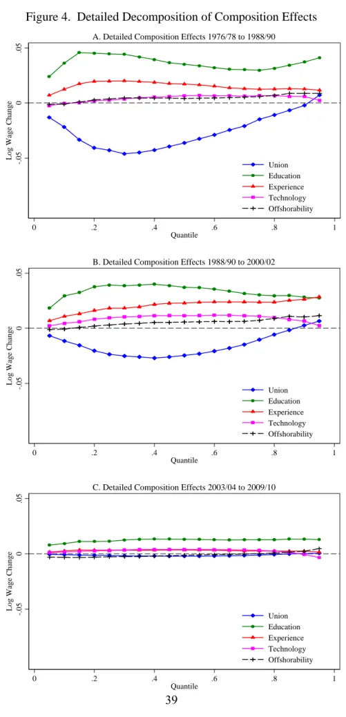
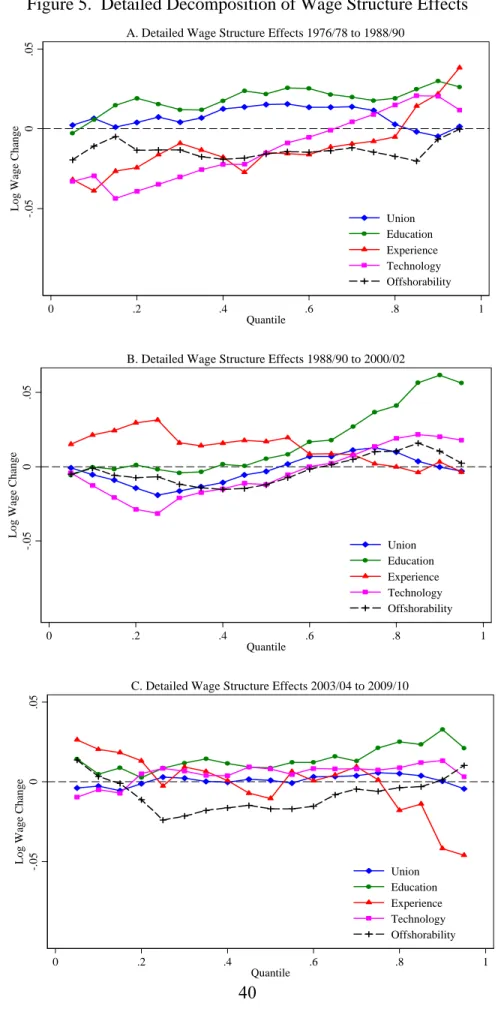
B. Detailed Decomposition Results
Figure 4 moves to the next step of the decomposition using RIF-regressions to apportion the
composition effect to the contribution of each set of covariates. Figure 5 does the same for the
wage structure effect. To simplify the presentation of the results, Figure 4 reports the composition
effect for five set of explanatory factors: union status, education, experience, offshorability and
technological change.38 The effect of the other covariates used in the RIF-regressions (race and
marital status) is generally small. We report it in Panel A of Table 4 under the “other” category.
For the sake of simplicity, we focus the discussion on the impact of each factor in the lower and
upper part of the distribution. Those are also summarized in terms of the 50-10 and 90-50 gaps
for the main analysis period (1988-90 to 2000-02) in Table 4.
First consider composition effects for the 1988-90 to 2000-02 period. With the notable exception
of unions, all factors have a larger impact on the 50-10 than on the 90-50 gap. The total
contribution of all factors other than unionization is 0.033 and -0.002 for the 50-10 and 90-50
gaps, respectively. Composition effects linked to factors other than unions thus go in the “wrong
direction” as they account for rising inequality at the bottom end while inequality is actually
rising at the top end of the distribution.
In contrast, composition effects linked to unions (the impact of de-unionization) reduce
in-equality at the low end (effect of -0.013 on the 50-10 gap) and increase inin-equality at the top end
(effect of 0.027 on the 90-50). Note that, as in a Oaxaca-Blinder decomposition, these effects on
the 50-10 and the 90-50 gap can be obtained directly by multiplying the 5.3 percent decline in the
unionization rate (Appendix Table A1) by the RIF-regression estimates of the union effects for
1988-90 (Appendix Table A4). The resulting effect of de-unionization accounts for 24 percent of
the total change in the 50-10 gap, and 30 percent of the change in the 90-50 gap. The magnitude
of these estimates is comparable to the relative contribution of de-unionization to the growth
in inequality estimated for the 1980s (see Freeman, 1993, Card, 1992, and DiNardo, Fortin and
Lemieux, 1996).
The results for the 1976-78 to 1988-90 period are reported in Figure 4a. Since unionization
declined more dramatically during in the 1980s (9.3 percentage point decline) than in the 1990s
(5.3 percentage point decline), the estimated contribution of de-unionization to inequality changes
is also larger during the earlier period. As in the 1990s, de-unionization has a larger and positive
38