Abstract—The Black-Scholes (B-S) model is the traditional
tool for giving a theoretical estimate of the price of European-style options. However, the basic assumptions on the assets and market made in the B-S model are ideal. Furthermore, a lot of factors which might affect the prices of options have not been considered in the B-S model. In this study, the genetic programming (GP) and support vector regression (SVR) are applied to forecast the prices of stock options by using the six basic factors in the B-S model and the other factors, such as the opening and closing prices, highest and lowest prices, trading volume, open interest etc., as the predictors. The performance of GP and SVR forecasting models are also compared to the B-S pricing model. The feasibility and effectiveness of the proposed approach are demonstrated by forecasting the closing prices of Taiwan Stock Exchange Capitalization Weighted Stock Index Options (TAIEX Options) from April 1, 2010 to March 29, 2013.
Index Terms—options, genetic programming, support vector
regression, Black-Scholes model
I. INTRODUCTION
HE financial investment is very popular as the economies developed rapidly. The options which provide the characteristic of making an infinite profit while taking a finite risk have become one of the major investing instruments. Investors can make more accurate investment decisions thus making higher returns on investment as well as avoiding risks, if the prices of options can be forecasted accurately. Therefore, the forecasting of options price has become a hot issue in the field of financial researches, and has received considerable attention from both researchers and practitioners.
The forecasting of options price is considered a challenging task since the prices are highly volatile, complex and dynamic. The Black-Scholes (B-S) model [1] is the traditional and important option pricing model for providing a theoretical estimate for the price of European-style options. However, the basic six assumptions on the assets and market
Manuscript received October 7, 2014; revised October 16, 2014. The authors would like to thank the Ministry of Science and Technology, Taiwan, ROC, for its support of this research under Contract No. MOST 103-2221-E-159-001.
Chih-Ming Hsu is with the Department of Business Administration, Minghsin University of Science and Technology, Hsinfong, Hsinchu 304, Taiwan, ROC (e-mail: cmhsu@ must.edu.tw).
Ying-Chi Fu, Yu-Chun Liu and Chun-Yi Peng are with the Institute of Management, Minghsin University of Science and Technology, Hsinfong, Hsinchu 304, Taiwan, ROC.
made while using the B-S option pricing formula are too ideal. In addition, the B-S model has not considered a lot of factors which might affect the prices of options, such as the opening and closing prices, highest and lowest prices, trading volume, open interest etc. Therefore, some approaches for tackling the problems of options price forecasting have been proposed by using the six basic factors in the B-S model and the other factors as the predictors, and/or by applying methodologies from various fields, e.g. data mining, neural networks and computational intelligence techniques [2]–[15].
This study applies the genetic programming (GP) and support vector regression (SVR) to forecast the prices of stock options based on the predictors consisting of the six basic factors in the B-S model and the other factors, including the opening and closing prices, highest and lowest prices, trading volume, and open interest. In addition, the forecasting performance of GP and SVR models are compared to the B-S options pricing model. The Taiwan Stock Exchange Capitalization Weighted Stock Index Options (TAIEX Options) are used to verify the feasibility and effectiveness of the proposed approach by forecasting the closing prices in the next trading day from April 1, 2010 to March 29, 2013.
II. METHODOLOGIES
A. Black-Scholes Model
The Black-Scholes (B-S) model [1] is one of the most important concepts in modern financial theory. It is considered the standard model for valuing options and is still widely used today. The six basic assumptions underlying the B-S model of calculating options pricing include (1) no dividends, (2) European return calculations, (3) efficient markets, (4) no commissions, (5) constant interest rates and (6) lognormally distributed returns. The values of call and put options for a non-dividend-paying underlying stock are calculated, respectively, by
rt
Ke d N S d N
C ( 1) ( 2) (1)
and
S d N Ke d N
P rt
) ( )
( 2 1
(2) where N() is the cumulative standard normal distribution; S
is the current price of the underlying stock; K is the option striking price; r is the risk-free interest rate; t is the time to maturity. In addition, the parameters d1 and d2 are determined,
respectively, by
t
t r
K S d
/2)
( ) /
ln( 2
1
(3)
Forecasting the Prices of TAIEX Options by
Using Genetic Programming and Support Vector
Regression
Chih-Ming Hsu, Ying-Chi Fu, Yu-Chun Liu, and Chun-Yi Peng
and
t d
d2 1 (4)
where is the volatility of returns of the underlying stock. B. Genetic Programming
Genetic programming (GP), inspired by biological evolution, is an evolutionary algorithm-based methodology that can automatically create computer programs to perform a user-defined task by genetically breeding a population of computer programs based on the principles of Darwinian natural selection and biologically inspired operations. The solution technique of GP is closely relates to genetic algorithms (GAs). However, the evolving individuals in GP are themselves computer programs, instead of fixed-length strings consisting of numbers, alphabetic letters, or symbols. The computer programs in GP are traditionally represented in memory as tree structures composed of terminal and function sets. The terminal set defines the terminal elements available for the branches of computer programs, such as independent variables, zero-argument functions, random constants, etc. On the other hand, the function set is a set of primitive functions available to each branch of computer programs, e.g. addition, square root, multiplication, sine, etc. Like other evolutionary algorithms, a fitness function is defined and used to explicitly or implicitly measure the fitness (adaptability) of individuals in the population. It specifies a desired goal in the search for GP. In addition, users must specify parameters including population size, maximum size of programs, crossover rate, mutation rate, etc., and set the termination criterion. The steps of GP are briefly described, as follows [16]–[18]:
Step 1: Generate an initial population appropriate to a problem subject to a pre-specified maximum size. Step 2: Evaluate computer programs based on a pre-defined
fitness function.
Step 3: Select a pool of programs from the population using a probability based on the fitness.
Step 4: Apply reproduction, crossover, mutation, and architecture-altering operations to the selected programs to produce the offspring.
Step 5: Replace the current population with the population of offspring based on a certain strategy to create the next generation.
Step 6: Designate the outcome as the final results when the termination criterion is satisfied. Otherwise, execute Steps 2 to 5 iteratively.
C. Support Vector Regression
Support vector regression (SVR) [19] is the application of the support vector machine (SVM) [20] to cases of function approximation or regression. SVR intends to construct a mathematical model to describe the functional dependence of d on X given a training data Q
k k k d
X , } 1
{ , where the input variable XkRn is an n-dimensional vector and the output
variable dkR is a real value. In order to resolve a non-linear regression problem, SVR utilizes a map to transform the original problem into a linear regression problem in a high dimensional feature space, and approximates a function of the form
0
0 ( )
) ( )
,
(X W w X w W X w
f T
m i
i
i
(5)where wi is the weight; W is the weight vector; i(X) is the feature; (X) is the feature vector; and w0 is the bias.
Vapnik [21] introduced the ε-insensitive loss function to evaluate the prediction error by
otherwise | ) , ( | | ) , ( | if 0 )) , ( , ( W X f d W X f d W X f d L . (6)
Therefore, the loss is expressed by Q i w X W d i T
i ( ) 0, 1,..., . (7)
Q i
d w X
W i i
T ,..., 1 , ) ( '
0
. (8)
Q i
i0, 1,...,
. (9)
Q i
i 0, 1,...,
'
. (10)
where i and '
i
are non-negative slack variables used to measure the errors above and below the predicted function, respectively, for each data point. The empirical risk minimization problem can then be defined as [21]–[22]
Q i i Q i i C W 1 ' 1 2 || || 21
. (11) subject to the constraints in (7)–(10), where C is a user
specified parameter for the trade-off between complexity and losses. The simplified dual form can be obtained, by constructing the Lagrangian in primal variables and making the partial derivatives with respect to the primal variables vanish at the saddle point for optimality, as follows
Maximize
Q i Q j j i j j i i Q i i i i i Q i i D X X K d L 1 1 ' ' 1 ' ' 1 ) , ( ) )( ( 2 1 ) ( ) ( ) ' , ( (12) subject to
Q i i i 1 ' 0 )( (13)
Q i
C
i , 1,...,
0 (14)
Q i
C
i , 1,...,
0'
(15) where K(Xi,Xj)(Xi)(Xj) is called the kernel
function. With the Lagrangian optimization done, the optimal weight vectors can be obtained as follows
) ( ) ˆ ˆ ( ) ( ) ˆ ˆ ( ˆ 1 ' 1 ' k n k k k i Q i i
i X X
W s
(16)
Where nsis the number of support vectors, and the index k only runs over support vectors. Finally, the optimal bias can be obtained by exploiting the Karush–Kuhn–Tucker (KKT) conditions [23]–[24], as follows
nus s i n k i i k k i us X X K d n w 1 1
0 ( , ) sign( )
1
ˆ (17)
where nus is the number of unbounded support vectors with Lagrangian multipliers satisfying 0iC and
ˆ ˆ
i
III. PROCEDURE OF FORECASTING OPTIONS PRICES
In this study, the genetic programming (GP) and support vector regression (SVR) are utilized to resolve problems inherent in forecasting options prices, where the six basic factors in the B-S model and the other factors which might affect the prices of stock options are considered the predictors. The proposed forecasting procedure is illustrated in Fig. 1 and is briefly described as follows:
Step 1: Collect the six basic factors in the B-S model and trading data of stock call options, including the price of underlying stock, striking price, risk-free interest rate, cash dividend yield, time to maturity, volatility of the underlying stock, opening price, closing price, highest price, lowest price, trade volume and open interest, in each trading day. Notably, the data are collected for the in-the-money at the first and second series, at-the-money, and out-of-the-money at the first and second series call options.
Step 2: Normalize the collected data into a range between 0 and 1 to avoid variables with larger numeric ranges from dominating those with smaller numeric ranges. Step 3: Construct GP and SVR forecasting models of options
prices.
Step 3-1: The normalized data are arranged into the form
) , ,..., ,
(x1 x2 xn y , and are then partitioned into training and test data based on a pre-specified proportion, e.g. 4:1, where x1 to xn are predictors
and y is the closing price of stock option in the next trading day.
Step 3-2: Apply GP and SVR to construct several forecasting models.
(1) Construct five GP models, called GPBS-In-2, GPBS-In-1,
GPBS-At, GPBS-Out-1 and GPBS-Out-2, to forecast the prices
for the in-the-money at the first and second series, at-the-money, and out-of-the-money at the first and second series call options, respectively, where the predictors x1 to xn are the six basic factors in the B-S
model. Similarly, five SVR models, called SVRBS-In-2,
SVRBS-In-1, SVRBS-At, SVRBS-Out-1 and SVRBS-Out-2, are
built to forecast the prices for the in-the-money at the first and second series, at-the-money, and out-of-the-money at the first and second series call options, respectively.
(2) Construct a GP model, called GPBS-All, to forecast the
prices for the in-the-money at the first and second series, at-the-money, and out-of-the-money at the first and second series call options where the predictors x1
to xn are the six basic factors in the B-S model. Similarly, an SVR models, called SVRBS-All, is built to
forecast the prices for the in-the-money at the first and second series, at-the-money, and out-of-the-money at the first and second series call options.
(3) Construct five GP models, called GPBS-OF-In-2,
GPBS-OF-In-1, GPBS-OF-At, GPBS-OF-Out-1 and GPBS-OF-Out-2,
to forecast the prices for the in-the-money at the first and second series, at-the-money, and out-of-the-money at the first and second series call options, respectively, where the predictors x1 to xn are
the six basic factors in the B-S model and the other
factors including the opening price, closing price, highest price, lowest price, trade volume and open interest. Similarly, five SVR models, called SVRBS-OF-In-2, SVRBS-OF-In-1, SVRBS-OF-At, SVRBS-OF-Out-1
and SVRBS-OF-Out-2, are built to forecast the prices for
the in-the-money at the first and second series, at-the-money, and out-of-the-money at the first and second series call options, respectively.
(4) Construct a GP model, called GPBS-OF-All, to forecast
the prices for the in-the-money at the first and second series, at-the-money, and out-of-the-money at the first and second series call options where the predictors x1
to xn are the six basic factors in the B-S model and the other factors including the opening price, closing price, highest price, lowest price, trade volume and open interest. Similarly, an SVR models, called SVRBS-OF-All,
is built to forecast the prices for the in-the-money at the first and second series, at-the-money, and out-of-the-money at the first and second series call options.
Step 4: Apply the B-S model to evaluate the prices for the in-the-money at the first and second series, at-the-money, and out-of-the-money at the first and second series call options.
Step 5: Evaluate the forecasting performances of GP and SVR models constructed in Step 3, and the B-S model used in Step 4 through the mean absolute percentage error (MAPE) and mean squared error (MSE).
IV. CASE STUDY
In this section, a case study on forecasting the closing prices of TAIEX Options of the spot month is presented to demonstrate the feasibility and effectiveness of the proposed forecasting procedure. The details of the case study and the procedure are described below.
A. Data Collection
TABLEI
PERIODS OF COLLECTING DATA AND FORECASTING HORIZONS
Case No.
Periods of collecting the data for
constructing forecasting models Forecasting horizons 1 2010/04/01~2011/03/31 2011/04/01~2011/06/30 2 2010/07/01~2011/06/30 2011/07/01~2011/09/31 3 2010/10/01~2011/09/31 2011/10/01~2011/12/31 4 2011/01/01~2011/12/31 2012/01/01~2012/03/31 5 2011/04/01~2012/03/31 2012/04/01~2012/06/30 6 2011/07/01~2012/06/30 2012/07/01~2012/09/31 7 2011/10/01~2012/09/31 2012/10/01~2012/12/31 8 2012/01/01~2012/12/31 2013/01/01~2013/03/31
B. Data Normalization
The collected data are normalized into a range between 0 and 1.
C. Constructions of GP and SVR Forecasting Models For each case in Table I, the data are randomly partitioned into training and test data groups, based on the proportion of 4:1. The GP algorithm is then applied to the training and test data to establish the GPBS-In-2, GPBS-In-1, GPBS-At, GPBS-Out-2,
GPBS-Out-2 and GPBS-All models as described in Section III.
Here, the Discipulus 4.0 (http://www.rmltech.com) software is employed where the fitness of a program is evaluated through the MSE. The termination criterion is that the generations without improvement have reached 100 and the remaining parameters are set as their default values in the software. The Discipulus 4.0 software is executed 5 times for each of the in-the-money at the first and second series, at-the-money, and out-of-the-money at the first and second series call options. Table II summarizes the best GP forecasting models selected from the 5 runs for case 1 in Table I. Similarly, GPBS-OF-In-2, GPBS-OF-In-1, GPBS-OF-At,
GPBS-OF-Out-1, GPBS-OF-Out-2 and GPBS-OF-All models where the
predictors are the six basic factors in the B-S model and the other factors including the opening price, closing price, highest price, lowest price, trade volume and open interest, as described in Section III, are constructed and summarized in Table III. Similarly, the SVR forecasting models as described in Section III can also be obtained and shown in Table IV and V. Here, LIBSVM 2.86 [25] with a radial basis function (RBF) kernel is utilized to implement the SVR technique. The optimal settings for parameters C, , and in SVR are determined by the grid-search approach [25]. In addition, the LIBSVM 2.86 utilizes the 10-fold cross-validation accuracy to calculate the overall MSE thus determining the final optimal model. Hence, the normalized data can be directly fed into the SVR tool to build the model instead of partitioning the data into the training and test data groups in advance.
TABLEII
INFORMATION ABOUT OPTIMAL GP FORECASTING MODELS FOR CASE 1 IN
TABLEI(PREDICTORS ARE BASIC FACTORS IN THE B-S MODEL)
Models’ names Training MSE
Test MSE
Training R2
Test R2
GPBS-In-2 0.058993 0.064769 0.51016 0.45809
GPBS-In-1 0.047715 0.040711 0.58070 0.65402
GPBS-At 0.036713 0.028582 0.72549 0.74292
GPBS-Out-1 0.025630 0.028385 0.81997 0.75284
GPBS-Out-2 0.024888 0.019691 0.80763 0.88846
GPBS-All 0.023026 0.022646 0.88823 0.88395
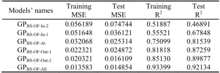
TABLEIII
INFORMATION ABOUT OPTIMAL GP FORECASTING MODELS FOR CASE 1 IN
TABLEI(PREDICTORS ARE BASIC FACTORS IN THE B-S MODEL AND OTHER FACTORS)
Models’ names Training MSE
Test MSE
Training R2
Test R2
GPBS-OF-In-2 0.056189 0.074744 0.51887 0.46891
GPBS-OF-In-1 0.051648 0.036121 0.55521 0.67848
GPBS-OF-At 0.032068 0.025314 0.75099 0.81539
GPBS-OF-Out-1 0.022321 0.024872 0.81818 0.87259
GPBS-OF-Out-2 0.020321 0.016109 0.85130 0.89877
GPBS-OF-All 0.013583 0.014854 0.93399 0.92134
TABLEIV
INFORMATION ABOUT OPTIMAL SVR FORECASTING MODELS FOR CASE 1 IN
TABLEI(PREDICTORS ARE BASIC FACTORS IN THE B-S MODEL) Models’ names Overall MSE Overall R2
SVRBS-In-2 0.055994 0.535634
SVRBS-In-1 0.039450 0.650397
SVRBS-At 0.050024 0.609386
SVRBS-Out-1 0.048294 0.652249
SVRBS-Out-2 0.038440 0.723557
SVRBS-All 0.018799 0.906678
TABLEV
INFORMATION ABOUT OPTIMAL SVR FORECASTING MODELS FOR CASE 1 IN
TABLEI(PREDICTORS ARE BASIC FACTORS IN THE B-S MODEL AND OTHER FACTORS)
Models’ names Overall MSE Overall R2
SVRBS-OF-In-2 0.062520 0.530361
SVRBS-OF-In-1 0.044611 0.631761
SVRBS-OF-At 0.027769 0.792306
SVRBS-OF-Out-1 0.024913 0.828414
SVRBS-OF-Out-2 0.033035 0.765719
SVRBS-OF-All 0.001031 0.994098
D. Pricing Options by the B-S Model
The B-S model is used to evaluate the prices for the in-the-money at the first and second series, at-the-money, and out-of-the-money at the first and second series call options based on the collected data of the six basic factors.
E. Evaluation of Forecasting Performance
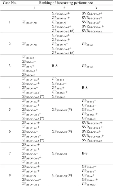
TABLEVI
THE BEST THREE FORECASTING MODELS BASED ON THE MAPE Case No. Ranking of forecasting performance
1 2 3
1 GPBS-OF-All
GPBS-OF-In-2+ GPBS-OF-In-1+ GPBS-OF-At+ GPBS-OF-Out-1+ GPBS-OF-Out-2 (#)
SVRBS-OF-In-2+ SVRBS-OF-In-1+ SVRBS-OF-At+ SVRBS-OF-Out-1+ SVRBS-OF-Out-2
2 GPBS-OF-All
GPBS-OF-In-2+ GPBS-OF-In-1+ GPBS-OF-At+ GPBS-OF-Out-1+ GPBS-OF-Out-2 (#)
GPBS-All
3
GPBS-In-2+ GPBS-In-1+ GPBS-At+ GPBS-Out-1+ GPBS-Out-2
B-S GPBS-All
4
GPBS-OF-In-2+ GPBS-OF-In-1+ GPBS-OF-At+ GPBS-OF-Out-1+ GPBS-OF-Out-2 (*)
GPBS-In-2+ GPBS-In-1+ GPBS-At+ GPBS-Out-1+ GPBS-Out-2
B-S
5
GPBS-OF-In-2+ GPBS-OF-In-1+ GPBS-OF-At+ GPBS-OF-Out-1+ GPBS-OF-Out-2 (*)
GPBS-OF-All (#)
GPBS-In-2+ GPBS-In-1+ GPBS-At+ GPBS-Out-1+ GPBS-Out-2
6
GPBS-OF-In-2+ GPBS-OF-In-1+ GPBS-OF-At+ GPBS-OF-Out-1+ GPBS-OF-Out-2 (*)
GPBS-OF-All (#)
SVRBS-OF-In-2+ SVRBS-OF-In-1+ SVRBS-OF-At+ SVRBS-OF-Out-1+ SVRBS-OF-Out-2
7
GPBS-OF-In-2+ GPBS-OF-In-1+ GPBS-OF-At+ GPBS-OF-Out-1+ GPBS-OF-Out-2
GPBS-OF-All B-S
8
GPBS-OF-In-2+ GPBS-OF-In-1+ GPBS-OF-At+ GPBS-OF-Out-1+ GPBS-OF-Out-2
GPBS-OF-All (#)
GPBS-In-2+ GPBS-In-1+ GPBS-At+ GPBS-Out-1+ GPBS-Out-2
The asterisk (*) denotes the paired t test for the models with rankings 1 and 2 is significant, and the number sign (#) represents the paired t test for the models with rankings 2 and 3 is significant (α=0.05).
TABLEVII
THE BEST THREE FORECASTING MODELS BASED ON THE MSE Case No. Ranking of forecasting performance
1 2 3
1 GPBS-OF-All (*) B-S (#) SVRBS-OF-All
2 GPBS-OF-All (*)
GPBS-OF-In-2+ GPBS-OF-In-1+ GPBS-OF-At+ GPBS-OF-Out-1+ GPBS-OF-Out-2
GPBS-All
3 GPBS-OF-All (*) B-S (#) GPBS-All
4 GPBS-OF-All (*) B-S (#) GPBS-All
5 GPBS-OF-All (*) SVRBS-OF-All (#)
GPBS-OF-In-2+ GPBS-OF-In-1+ GPBS-OF-At+ GPBS-OF-Out-1+ GPBS-OF-Out-2
6 GPBS-OF-All (*) B-S GPBS-All
7 GPBS-OF-All B-S (#) SVRBS-OF-All
8 GPBS-OF-All (*) B-S (#) SVRBS-OF-All
The asterisk (*) denotes the paired t test for the models with rankings 1 and 2 is significant, and the number sign (#) represents the paired t test for the models with rankings 2 and 3 is significant (α=0.05).
V. CONCLUSION
In this study, the genetic programming (GP) and support
vector regression (SVR) are applied to design the forecasting models for the prices of stock call options where the predictors comprise the six basic factors in the B-S model and the other factors, including the opening price, closing price, highest price, lowest price, trade volume and open interest. The feasibility and effectiveness of the proposed approach are demonstrated via a case study in which the closing prices of Taiwan Stock Exchange Capitalization Weighted Stock Index Options (TAIEX Options) from April 1, 2010 to March 29, 2013 are forecasted. Furthermore, the GP and SVR forecasting models are compared to the traditional B-S pricing model. The experimental results indicate that the GP technique can provide the best models while evaluating the forecasting performance either based on the MAPE or based on the MSE, for all cases. In addition, the forecasting performance of models which only take the six basic factors in the B-S model as the predictors can be significantly improved by considering the other factors, such as the opening price, closing price, highest price, lowest price, trade volume and open interest to be the input variables.
REFERENCES
[1] F. Black, and M. Scholes, “The pricing of options and corporate liabilities,” Journal of Political Economy, vol. 81, no. 3, pp. 637−654, 1973.
[2] G. Meissner, and N. Kawano, “Capturing the volatility smile of options on high-tech stocks−A combined GARCH-neural network approach,
Journal of Economics and Finance, vol. 25, no. 3, pp. 276−296, 2001.
[3] C. A. Zapart, “Beyond Black–Scholes: a neural networks-based approach to options pricing,” International Journal of Theoretical and Applied Finance, vol. 6, no. 5, pp. 469−489, 2003.
[4] V. S. Tzastoudis, N. S. Thomaidis, and G. D. Dounias, “Improving neural network based option price forecasting,” Lecture Notes in
Computer Science, vol. 3955, pp. 378-388, 2006.
[5] C.-H. Tseng, S.-T. Cheng, Y.-H. Wang, and J.-T. Peng, “Artificial neural network model of the hybrid EGARCH volatility of the Taiwan stock index option prices,” Physica A: Statistical Mechanics and its Applications, vol. 387, no. 13, pp. 3192−3200, 2008.
[6] Y.-H. Wang, “Using neural network to forecast stock index option price: a new hybrid GARCH approach,” Quality & Quantity, vol. 43, no. 5, pp. 833−843, 2009.
[7] X. Liang, H.-S. Zhang, J.-G. Mao, and Y. Chen, “Improving option price forecasts with neural networks and support vector regressions,”
Neurocomputing, vol. 72, no. 13–15, pp. 3055–3065, 2009.
[8] M.-H. Chiang, and H.-Y. Huang, “Stock market momentum, business conditions, and GARCH option pricing models,” Journal of Empirical Finance, vol. 18, no. 3, pp. 488−505, 2011.
[9] L. Stentoft, “American option pricing with discrete and continuous time models: an empirical comparison,” Journal of Empirical Finance, vol. 18, no. 5, pp. 880−902, 2011.
[10] C.-P. Wang, S.-H. Lin, H.-H. Huang, and P.-C. Wu, “Using neural network for forecasting TXO price under different volatility models,”
Expert Systems with Applications, vol. 39, no. 5, pp. 5025−5032, 2012.
[11] H.-Y. Zhang, “Research on factors influencing European option price by using hybrid neural network,” Advances in Intelligent and Soft
Computing, vol. 144, no. 10, pp. 247−252, 2012.
[12] H. Park, and J. Lee, “Forecasting nonnegative option price distributions using Bayesian kernel methods,” Expert Systems with Applications, vol. 39, no. 18, pp. 13243−13252, 2012.
[13] W. I. Chuang, T. C. Huang, and B. H. Lin, “Predicting volatility using the Markov-switching multifractal model: Evidence from S&P 100 index and equity options,” North American Journal of Economics and
Finance, vol. 25, pp. 168–187, 2013.
[14] H. Park, N. Kim, and J. Lee, “Parametric models and non-parametric machine learning models for predicting option prices: Empirical comparison study over KOSPI 200 Index options,” Expert Systems with Applications, vol. 41, no. 11, pp. 5227−5237, 2014.
[16] J. R. Koza, M. A. Keane, M. J. Streeter, M. J., W. Mydlowec, J. Yu, and G. Lanza, Genetic programming IV: Routine human-competitive
machine intelligence. New York: Springer, 2005.
[17] I. Ciglarič, and A. Kidrič, “Computer-aided derivation of the optimal mathematical models to study gear-pair dynamic by using genetic programming,” Structural and Multidisciplinary Optimization, vol. 32, no. 2, pp. 153–160, 2006.
[18] J. R. Koza, M. J., Streeter, and M. A. Keane, “Routine high-return human-competitive automated problem-solving by means of genetic programming,” Information Sciences, vol. 178, no. 23, pp. 4434–4452, 2008.
[19] C. Cortes, and V. Vapnik, “Support-vector networks,” Machine
Learning, vol. 20, no. 3, pp. 273–297, 1995.
[20] H. Drucker, C. J. C. Burges, L. Kaufman, A. Smola, and V. Vapnik, “Support vector regression machines,” in Advances in Neural
Information Processing Systems, vol. 9, M. C. Mozer, M. I. Jordan, and
T. Petsche, Eds., Cambridge, MA: MIT Press, 1997, pp. 155–161. [21] V. Vapnik, Statistical Learning Theory. New York: Wiley, 1998. [22] V. Vapnik, The Nature of Statistical Learning Theory. New York:
Springer-Verlag, 1995.
[23] W. Karush, “Minima of Functions of Several Variables with Inequalities as Side Constraints,” Master Thesis, Department of Mathematics, University of Chicago, Chicago, IL, 1939.
[24] H. Kuhn and A. Tucker, “Nonlinear programming,” in Proceedings of the 2nd Berkeley Symposium on Mathematical Statistics and
Probabilistics, 1951, pp. 481–492.
[25] C.-C. Chang and C.-J. Lin, “LIBSVM: a library for support vector machines,” ACM Transactions on Intelligent Systems and Technology, vol. 2, no. 3, pp. 2:27:1–27:27