ON ENHANCING DATA UTILITY IN K-ANONYMIZATION FOR DATA
WITHOUT HIERARCHICAL TAXONOMIES
Mohammad Rasool Sarrafi Aghdam1 and Noboru Sonehara2 1
The Graduate University for Advanced Studies, Informatics Department [email protected]
2
National Institute of Informatics [email protected]
ABSTRACT
K-anonymity is the model that is widely used to protect the privacy of individuals in publishing micro-data. It could be defined as clustering with constrain of minimum k tuples in each group. K-anonymity cuts down the linking confidence between sensitive information and specific individual by the ration of 1/k. However, the accuracy of the data in k-anonymous dataset decreases due to information loss. Moreover, most of the current approaches are for numerical attributes or in case of categorical attributes they require extra information such as attribute hierarchical taxonomies which often do not exist. In this paper we propose a new model, based on clustering, defining the distance between tuples including numerical and categorical attributes which does not require extra information and present the SpatialDistance (SD) heuristic algorithm. Comparisons of experimental results on real datasets between SD algorithm and existing well-known algorithms show that SD performs the best and offers much higher data utility and reduces the information loss significantly.
KEYWORDS: Anonymization, Data quality, Data mining, Algorithm, Security
1 INTRODUCTION
Most of the service providers in real and cyber world collect and store large amount of data on individuals as their normal process of operations. For example hospitals collect and keep the registration information in addition to the medical record information of their patients. In these collected data there might exist some correlation between the quasi-identifier (QID) attributes (e.g., gender and ZIP code) and private sensitive attributes (e.g., disease). For instant, people living in specific region might have a tendency of a
particular disease. Investigation on the collected data and discovering this kind of correlation is very helpful and interesting for researchers. However, publishing the collected data containing private sensitive information or sharing it with the third parties would bring up some privacy concerns even if the name and social security number of individuals, which is called the identifying information, are discarded before releasing the data.
There are a lot of external data sources accessible to everyone through Internet including the QID and identifiers attribute (e.g., Voter Registration dataset). Due to the existence of QID attributes in the released dataset, the released dataset could be linked to the external dataset. This established link could result in re-identifying the individuals uniquely and disclosure of their private sensitive information. Technically this is known as
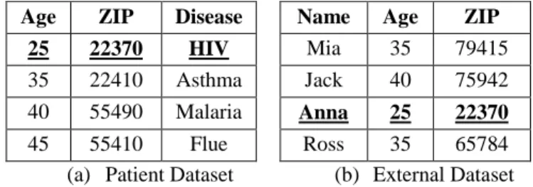
“linking attack” [1], [3], [4]. A sample of linking attack between the patient dataset released by a hospital and external dataset is illustrated in Table 1 in which the privacy of Anna is violated.
Table 1. Linking Attack between (a) Patient Dataset and (b) External Dataset
Age ZIP Disease
25 22370 HIV
35 22410 Asthma
40 55490 Malaria
45 55410 Flue
Name Age ZIP
Mia 35 79415
Jack 40 75942
Anna 25 22370
Ross 35 65784
(a) Patient Dataset (b) External Dataset
Based on the study on US population in [2],
US population. Hence, for exercising data mining while protecting the privacy of individuals, privacy preserving data mining (PPDM) concept has been proposed [5]. One of the approaches in PPDM is k-anonymity model which is proposed by Samarati and Sweeney [1], [3], [4]. K-anonymity protects the privacy of individuals by modifying the values of QID attributes through generalization so that each record in the released dataset is indistinguishable from at least k-1 other records within the same dataset. The k factor is the anonymization degree and it shows the desired privacy level. The linking confidence between the k-anonymous released dataset and the external dataset will reduce by 1/k ratio therefore it can be concluded that the privacy of individuals is protected to some extent. Table 2 represents the 2-anonymous patient dataset which was originally shown in Table 1(a).
Table 2. 2-Anonymous Patient Dataset
Age ZIP Disease
25 ~ 35 22*** HIV
25 ~ 35 22*** Asthma
40 ~ 45 554** Malaria
40 ~ 45 554** Flue
Proportionally by increasing the k value the privacy protection will be better. However, by comparing the Table 1(a) with Table 2, it is very clear that due to the modification of original data in generalization process the k-anonymous dataset loses its accuracy and some information loss occurs. The main challenge in k-anonymization is to minimize the information loss and obtain the maximum utility k-anonymous dataset. The problem of optimal k-anonymization and achieving k-anonymity with minimal loss of information is shown to be NP hard problem [6], [7], [8]. Also, there exists a tradeoff relationship between the privacy level and the quality of anonymized-data. One of the possible approaches to solve the high information loss problem is through the heuristic algorithms [9], [10], [11], [12]. In addition, real world datasets contain numerical and categorical data. As a matter of fact
most of the QID attributes in micro-data are assumes to be categorical [13]. This combination of different type of data makes the anonymization process rather complicated and very often results in inefficient anonymization as most of the existing methods are concentrated on numerical data or in case of categorical data they require additional information such as hierarchical taxonomies which mostly do not exist in real life applications.
In this work, at first we introduce some of the terminologies and definitions. Then we study some of the information quality metrics and introduce the measurement on information loss which we have used to evaluate our algorithm on k-anonymity. We propose a new model based on clustering and distance calculation between tuples for numerical and categorical attributes and based on the proposed model we present the SpatialDistance (SD) greedy algorithm. At the end we evaluate the SD algorithm and compare it with other existing famous algorithms with respect to information loss and utility of anonymized data.
2 PRELIMINARY DEFINITIONS
Considering the original dataset T which contains the information on each individual in n attributes {A1,…,An} the main terminologies are defined as below.
Quasi-Identifier attributes: A quasi-identifier
is a set of attributes in dataset T which can potentially join with external datasets to reveal private information of individuals. For example Age and ZIP attribute set in Table 1(a) is a quasi-identifier which can link the patient dataset to the external dataset and reveal some private information.
Equivalent class: An equivalent class E of
dataset T is a set of all tuples in T containing identical values with respect to QID attributes. For instant tuple 1 and 2 in Table 2 form an equivalent class (E1) with respect to attributes Age and ZIP.
K-anonymity: A dataset T is said to be
they size of every equivalent class is greater or equal to pre-defined k value.
3 INFORMATION QUALITY METRICS IN
K-ANONYMITY
One of the common ways in order to evaluate an algorithm in k-anonymization is to measure the quality of anonymized data and the information loss. There are various definitions regarding the information quality metrics. For instant, Minimal Distortion (MD) [14] is a single attribute measure and it defines the information loss as number of instances which are made indistinguishable. The Discernibility Metric (DM) [15] assigns penalty to each record based on the number of records indistinguishable from that record in anonymized table. The DM metric defines information loss for generalization and suppression, which can be expressed mathematically as follows.
g,k ∑ | |
s.t.| k|
∑ | || |
s.t.| k|
(1)
In this expression E is the equivalent class and | | is the size of the original dataset. The first sum calculates the information loss for generalized tuples and the second sum computes the information loss due to suppression. The information loss in both MD and DM is defined based the size of the group that the record is generalized and even though the DM is more accurate than MD, in k-anonymization methods which are near optimum, the size of the groups are close to k value which makes these metrics less practicable.
The more accurate metric is the Normalized Certainty Penalty (NCP) [16], which defines information loss due to generalization for both numerical and categorical attributes. For numerical attributes the NCP of a cell on numerical attribute Ai that lays on equivalent class G is defined as:
PAi
a Ai inAi
a Ai inAi
(2)
In case of categorical attributes, the NCP of the equivalent class G in Ai attribute is defined as follows.
PAi {
, ard u 1 ard u
ard i , therwise (3)
Where, ard u is the number of distinct values of Ai in G and ard i is the total number of distinct values of attribute Ai. By normalizing the total NCP between zero and one, the utility of anonymized data could be defined as follows.
Data Utility = 1 – NCPTotal (4) For information loss measurement, it is very important to choose the right measurement metric. In work [17] the information loss and data utility is measured using NCP, however NCP only measures the information loss due to generalization and in [17] both suppression and generalization have been used for anonymization. Therefore the evaluation results may not be reliable and precise because the information loss due to suppression is not calculated.
In k-anonymity the two commonly applied techniques are generalization and suppression which are technically defined as recoding the values in the original table [1]. Generalization is actually replacing an element in the original table with a general value that includes that element and suppression is replacing the element in the original table with null value. There are three main methods of generalization, global recoding, multidimensional and local recoding.
higher domain. This may cause over generalization of a table, which results in very high information loss. On the other hand in multidimensional and local recoding, the generalization is taking place at cell levels [7], [8], [10], [11]. They do not cause over generalization which lead to more flexible generalization and have the potential of less information loss. Multidimensional recoding problem is studied in [19] and it suggested an efficient partitioning method for multidimensional recoding anonymization. Mondrian is a heuristic algorithm with top down approach. It considers that all the data are sorted along all the attributes and starting from the whole dataset as a single group it splits the group into segments considering that the minimum group size is k [19]. However it is not practical in most of cases involving categorical attributes because this method requires the total order for each attribute domain and in categorical attributes there is no meaningful order. The work in [16] introduces utility based anonymization through local recoding generalization. It introduces a new quality metric that calculates the information loss due to generalization for both numerical and categorical attributes and actually uses this quality metric for clustering the tuples. However this method assumes that for every categorical attribute in the dataset the hierarchical structure is defined and exist which is not so realistic considering real life applications. In our work we consider local recoding generalization, as it is more flexible and efficient with the possibility of lower information loss.
4 PROPOSED MODEL
As it was mentioned in introduction, the main issue in k-anonymity is the huge information loss that occurs in anonymization process and causes the original data to lose its accuracy. Moreover even though the real datasets are consist of numerical and categorical attributes, current methods are mainly consider the numerical data or if they consider categorical data they require additional information such as attribute
hierarchical taxonomies which mostly do not exist in real life applications.
In order to increase the utility of anonymized data for real datasets consisting of numerical and categorical data, without the need of additional information on attributes in the dataset, we are introducing a new approach based on clustering using distance calculation between the tuples for anonymization through local recoding generalization. In our approach, the distance is actually represents the information loss and in order to select and place the closest tuples into same equivalent class the distance between tuples need to be calculated. The distance calculation differs depending on the type of attribute. In this section we will be discussing the distance definition between tuples for numerical and categorical attributes.
4.1Distance Definition for Numerical and Categorical Attributes
Let’s consider the original dataset T with quasi identifier attributes (A1,…,Aj) which consists of numerical and categorical attributes. The dataset T with i tuples and jattributes is mapped as i points in j dimensional Euclidian space.
The distance measurement between tuples t1 and t2 with values of x1 and x2 with respect to attribute Ai assuming that Ai is a numerical attribute is defined as t1,t Ai a | 1- |
Ai – inAi
where | - | is the absolute value and
a Ai – inAi is the range in attribute Ai. Therefore the total distance between two tuples with respect to numerical attributes in a dataset with n QID numerical attributes (A1,…,An) is defined as below.
(t1,t ) otal ∑
n
i 1
| 1Ai Ai|
a Ai inAi
(5)
continuous, some of the previous works [e.g., 12, 16] defined the distance with the help of hierarchical taxonomies. However, the attribute hierarchical taxonomies do not exist or defined in real life applications. In our model we define the distance between two tuples in categorical attributes based on the context and observation probability of the values in each attribute.
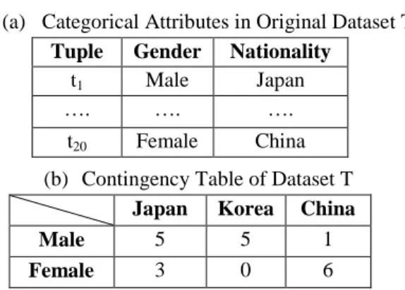
The first step in this approach is to build the contingency table which basically is the matrix format representation of the original table. The contingency table shows the frequency distribution of the variables and assists to measure the observation probability for each value of categorical attribute Aj. Then, the similarity between y1, the value of the first tuple (t1) in Aj, and the rest of the values in other tuples of Aj could be assessed. The values in Aj which have closer observational probability to y1 are defined as more similar and vice versa. Finally with the help of the similarity measurement between y1 and the rest of the values in other tuples of Aj the distances between t1 and the rest of the tuples in Aj could be defined. For example, the dataset T with two categorical attributes and its contingency table is shown in Figure 1.
(a) Categorical Attributes in Original Dataset T
Tuple Gender Nationality
t1 Male Japan
…. …. ….
t20 Female China
(b) Contingency Table of Dataset T Japan Korea China
Male 5 5 1
Female 3 0 6
Figure 1. (a) Categorical Attributes in Dataset T and (b) its Contingency Table
Regarding the similarity measurement in categorical attributes using contingency table we define the following terms.
Definition 1: The distance between identical
values is considered as zero. Therefore if the cardinality of a categorical attribute is one then
there is no need to measure the similarity for that attribute.
Definition 2: If the cardinality of a categorical
attribute is equal to two then the distance between the two values is defined as maximum distance equal to one.
Based on these definitions, only for categorical attribute with cardinality more than two the similarity measurement is required for distance definition.
In Figure 1, there are two categorical attributes, Sex = {Male, Female} with cardinality two and Nationality = {Japan, Korea, China} with cardinality three. Based on Definition 2 the distance between Male and Female is already defined as one therefore the contingency table is formed and shown in Figure 1(b) based on the original table in Figure 1(a) for similarity measurement between the values in Nationality attribute. As shown in Figure 1(a) the values of Sex and Nationality attributes in t1 are {Male} and {Japan}. By indicating the values in t1 we start the similarity measurement for attribute with minimum cardinality more than two, which in this example is Nationality attribute.
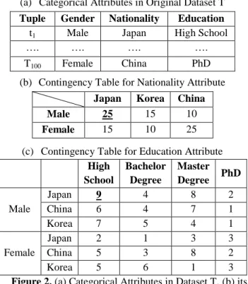
In this case since there are only two categorical attributes having one contingency table is enough. However, if there are more categorical attributes in dataset T, in order to find the similarities between the values in the next higher cardinality attribute, we add the next higher cardinality attribute to the existing contingency table after similarity measurement for lower cardinality attributes is done. An example with having more than one contingency table is shown in Figure 2.
(a) Categorical Attributes in Original Dataset T
Tuple Gender Nationality Education
t1 Male Japan High School
…. …. …. ….
T100 Female China PhD
(b) Contingency Table for Nationality Attribute
Japan Korea China
Male 25 15 10
Female 15 10 25
(c) Contingency Table for Education Attribute High
School
Bachelor Degree
Master Degree PhD
Male
Japan 9 4 8 2
China 6 4 7 1
Korea 7 5 4 1
Female
Japan 2 1 3 3
China 5 3 8 2
Korea 5 6 1 3
Figure 2. (a) Categorical Attributes in Dataset T, (b) its Contingency Table for Nationality Attribute and (c) The
Contingency Table for Education Attribute Similarity Measurement
In order to evaluate the similarity between values of an attribute, the total number of tuples in each row in each contingency table as shown in Table 3 needs to be calculated. Because the k-value is pre-defined and it determines the minimum number of tuples in every cluster, therefore if the total number of tuples in every row of the contingency table is greater than or equal to the pre-defined k value then the similarities are measured with respect to the total number of tuples in that row only, otherwise other rows in that specific attribute needs to be considered. In this example the k value is considered to be three and the total number of tuples in Male row in Table 3 is greater than k value. However if it was not, the Female row also would be considered for similarity measurement between the values in Nationality attributes.
Table 3. Contingency Table of Dataset T and the Total Number of Tuples in Each Row
Japan Korea China Total No. of Tuples
Male 5 5 1 5+5+1 = 11 k=3
Female 3 0 6 3+0+6 = 9 k=3
The similarity factor is actually defined using the conditional probability. Considering a dataset T with two categorical attributes M= { m1,…,mi } and N= { n1,…,nj }, the similarity factor for the values of attribute M when i , i , L and the total number of tuples in mK is more than k value, is defined as:
nL mk |nL| m
(|n1| |n |)m (6)
In the expression (6) the numerator |nL| m is the number of tuples which have the value of mK in M attribute and nL in N attribute. (|n1| |n|)m is the total number of tuples in attribute N with the value of mK in M attribute. This expression can be expanded for datasets with more than two categorical attributes.
By utilizing the above expression all the similarity factors or the observation probabilities for all the values in attribute N with respect to mK in M attribute can be calculated. Therefore the similarity between the value of t1 in attribute N and other values in N could be defined as the closer the nL mk is to n1 mk , the more similar nL is to n1. The similarity between the values of Nationality= {Japan, Korea, China} in Table 3 with respect to Male value in Gender attribute is
calculated as,
a an ale | a an| || orea a an|| ale| | ale 11 ,
orea ale 11 and hina ale 111. So now by having the similarity factors we can conclude that since a an ale is closer to ale than
hina ale then Japan is more similar to Korea. After the similarity measurement and knowing the most and least similar values to the value of t1 in Nationality attribute in this example, the distances can be defined.
maximum equal to one so we have
ale, emale 1. Moving on to the next minimum cardinality attribute (Nationality attribute) we start the distance definition between the value of t1 and the least similar value to the value of t1 which is a an, hina and define the distance as the minimum distance calculated in the lower cardinality attribute, which in this case is the distance between Male and Female in Gender attribute, over the cardinality of the attribute (Nationality attribute) minus one which basically indicates the number of distances to define in that
particular attribute. Therefore
a an, hina in Att.
| ard ationalit |-1
1
. In Nationality attribute the second least similarity is between Japan and Korea and a an, orea is defined as a an, hina divided by | ard ationalit |-1 . Therefore
a an, orea a an, hina 14 .In this example, finally by having ale, emale ,
a an, hina and a an, orea defined, the total distance between t1 and other tuples in dataset T regarding categorical attributes can be calculated as the sum of the ale, emale and
a an, or orea .
Considering the original dataset T with the numerical attributes { 1, , m} and categorical attributes { 1, , }, the total distance between two tuples t1 and t2 is defined as a sum of the distances in numerical and categorical attributes.
t1,t ∑ ( t1[ i],t [ i] ) i 1,…,m
∑ (t1[ ],t [ ]) 1,…,n
(7)
4.2SpatialDistance (SD) Greedy Algorithm Utilizing the introduced model on similarity and distance definition, we are able to obtain the total distance between any two tuples in the dataset. In this section we introduce a greedy algorithm with bottom-up approach called SpatialDistance (SD) algorithm which considers every tuple as a point in the Euclidean space. SD seeks to find and
cluster the k-1 closest tuples to the first tuple (t1) in dataset and place the tuples in the same equivalent class for anonymization through local recoding generalization.
In SD, the original dataset is sorted based on the maximum cardinality attribute and the total distances between t1 and other tuples are calculated using the introduced model. Then t1 and the tuple with minimum distance are moved to
Merge clause and deleted from T. The number of
tuples in Merge clause must be greater or equal to pre-defined k value, therefore if the group size in
Merge clause is less than k then more tuples need
to be added to Merge clause. So the center point (tc) of the tuples in Merge clause will replace t1 in original dataset and the distance between tc and the rest of the tuples in dataset T is calculated, so the tuple with minimum distance is moved to Merge clause and deleted from original dataset T.
Input: Original dataset T & K value Output: K - anonymous table T' Method:
1: Sort T Asc on Max_ Cardinality_Attribute 2: IF Atti is Categorical_ Att
Contingency table constructed & Define distances 3: WHILE |dataset T| > K DO {
Move t1 into Merge clause & Delete from T
WHILE |Merge clause| < K {
FOR i = 1 to |dataset T| DO{
Calculate DistanceTotal between t1 or tc & other tuples }
Move tuple (ti) with min (di) into Merge clause &
Delete ti from T & Calculate new tc }
Save Merge clause as Ej & Clear Merge & Update Contingency tables}
4: WHILE |dataset | && |dataset | ≠ {
FOR k = 1 to |dataset T| DO { FOR b = 1 to |Eb| DO {
Calculate tc of Eb & Calculate DistanceTotal between tc & tk }
Move tuple (tk) with min (db) into Eb & Delete tk from T }}
5: Generalize all E & Publish table T'
Figure 3. Pseudo Code of SD Algorithm
Merge clause is greater or equal to k value. Once
the number of tuples in Merge clause is equal or greater than k value the tuples in Merge clause considered as an equivalent class and anonymized through local recoding anonymization.
At the end if there is still some tuples left in the original dataset (number of tuples is less than k value), these remaining tuples will have to join one of the equivalent class with minimum distance. Therefore the tc of each equivalent class is obtained and the tuple will be added to the equivalent class with minimum distance. This process will repeat until there is no tuple left in original dataset T. The pseudo code for the SD algorithm is shown in Figure 3.
5 EXPERIMENTAL RESULTS
As we have mentioned earlier one of the ways to evaluate an algorithm on k-anonymity is to measure the information loss and the utility of anonymized data.
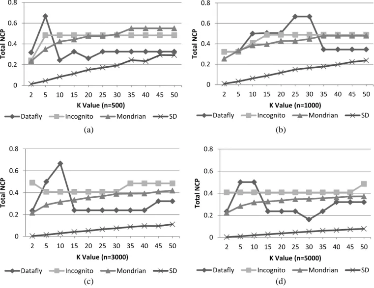
Therefore in order to evaluate our SD algorithm we have calculated the information loss using the total Normalized Certainty Penalty (NCP) metric and the utility of anonymized data for different anonymity degree (k = 2, 5, 10, 15, 20, 25, 30, 35, 40, 45, 50) on different size of datasets (n = 500, 1000, 3000, 5000) and compared the results with existing well-known algorithm such as Incognito, Datafly and Mondrian algorithms [18], [14], [19].
(a) (b)
(c) (d)
Figure 4. Information Loss Comparison between Mondrian, Incognito, Datafly and SD Algorithms
Regarding the sample dataset, we have used the Adult dataset from UCI Machine Learning
Repository, which contains census data and has become a benchmark for k-anonymity [22]. For
0 0.2 0.4 0.6 0.8
2 5 10 15 20 25 30 35 40 45 50
To
tal N
CP
K Value (n=500)
Datafly Incognito Mondrian SD
0 0.2 0.4 0.6 0.8
2 5 10 15 20 25 30 35 40 45 50
To
tal N
CP
K Value (n=1000)
Datafly Incognito Mondrian SD
0 0.2 0.4 0.6 0.8
2 5 10 15 20 25 30 35 40 45 50
To
tal N
CP
K Value (n=3000)
Datafly Incognito Mondrian SD
0 0.2 0.4 0.6 0.8
2 5 10 15 20 25 30 35 40 45 50
To
tal N
CP
K Value (n=5000)
the simulation of Mondrian, Incognito and Datafly algorithms we have used UTD anonymization toolbox which is available online [23]. In general because of the tradeoff relationship between the privacy (anonymity degree k) and data utility, by increasing the k value the information loss (total NCP) is supposed to be increasing. By looking at Figure 4, it is clear that the total NCP of the SD algorithm for the range of k values is much less than other algorithms while the same privacy level (k value) is kept. Also as the size of the dataset increases (Figure 4(d)) the difference between SD
and other algorithms especially in larger k values becomes more significant and the trend of total NCP in SD turns smoother. This advantage of SD algorithm in reducing the information loss significantly while maintaining the anonymity degree would result in a very high utility for anonymized data.
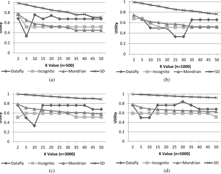
The comparison on utility of anonymized data using the expression (4) between SD, Mondrian, Incognito and Datafly algorithms are shown in Figure 5.
(a) (b)
(c) (d)
Figure 5. Comparison on Utility of Anonymized data between Mondrian, Incognito, Datafly and SD Algorithms
By looking at the SD results in Figure 5 the tradeoff relationship between the privacy and data utility is very obvious that by increasing the k value the utility is decreasing. However, in other algorithms such as Incognito and Datafly the tradeoff relationship is not very clear due to the
over generalization or inefficient clustering that caused high information loss even in small k values. As it was expected by having the result on total NCP measurement, the utility of anonymized data in SD algorithm is much higher than other algorithms in the range of k values as it is shown
0 0.2 0.4 0.6 0.8 1
2 5 10 15 20 25 30 35 40 45 50
Uti
li
ty
K Value (n=500)
Datafly Incognito Mondrian SD
0 0.2 0.4 0.6 0.8 1
2 5 10 15 20 25 30 35 40 45 50
Uti
li
ty
K Value (n=1000)
Datafly Incognito Mondrian SD
0 0.2 0.4 0.6 0.8 1
2 5 10 15 20 25 30 35 40 45 50
Uti
li
ty
K Value (n=3000)
Datafly Incognito Mondrian SD
0 0.2 0.4 0.6 0.8 1
2 5 10 15 20 25 30 35 40 45 50
Uti
li
ty
K Value (n=5000)
in the Figure 5. Also by investigating on the clusters made using SD algorithm, it is found that the outlier tuples are in the groups in which the total number of tuples are more than k value. This means that the outliers are provided with more privacy compare to regular tuples.
5.1SD Complexity Analysis
The computational complexity in SD actually depends on the k value which is defined for the dataset. The range of the k value is considered as
1 n. There are two primitive operations in SD the first one is calculating all the distance between t1 or tc with the rest of the tuples and the second operation is comparing the calculated distances. The worst case scenario for computational complexity is when k value is maximum (k n ⁄ ). Considering the maximum number of iterations to make one group with k tuples is k-1, therefore the complexity of the algorithm in the worst case is n . However, even though the number of tuples in datasets for real life applications is huge but the selected k value, which represents the desired privacy level, is not maximum or even close to it. It is mostly selected in a much smaller range. Therefore the computational complexity is much lower in real life applications.
6 CONCLUSION
In this paper, we have studied the most major issue in k-anonymity model which is the low data utility in k-anonymous table. We have also pointed out the issue in real life applications where the real datasets are a combination of numerical and categorical attributes and yet most of the existing models are considering only the numerical attributes or for categorical attributes they depend on the hierarchical taxonomies or some additional information which are mainly do not exist or defined. Then we have proposed a new model in which the distance between two tuples including numerical and categorical attributes can be obtained and k-anonymity through efficient clustering and local recoding generalization could be achieved. We Presented SD algorithm based on
the proposed model and finally evaluated our algorithm and compared the simulation results with respect to information loss and data utility with other well-known algorithms which show clearly that SD offers much higher utility for anonymized data and the information loss due to generalization is significantly reduced in addition of being independent of attribute hierarchies or any additional information.
7 PREFERENCES
1. L. weene , “k-Anonymity: A Model for Protecting
Privac ,” Int. ournal of Uncertaint , uzziness and
Knowledge-Based Systems, vol. 10, 2002, pp. 557– 570.
2. P. olle, “Revisiting the Uniqueness of im le
demogra hics in the U Po ulation,” Worksho on
Privacy in the Electronic Society (WPES), October 30, 2006, Alexandria, Virginia, USA, pp. 77–80. 3. P. Samarati and L. Sweeny, "Generalizing data to
provide anonymity when disclosing information." In: Proceedings of the ACM SIGACT-SIGMOD-SIGART symposium on principles of database
s stems P ’98 , A , . 188–188.
4. P. amarati,” Protecting Res ondents’ Identities in
icrodata Release,”I rans nowledge and
Data Eng., vol.13, no. 6, NOV./Dec. 2001, pp. 1010–1027.
5. R. Agrawal and R. rikant. “Privac -preserving
data mining,” A I Record, vol. 9,
2000, pp. 439–450.
6. G. Aggarwal, T. Feder, K. Kenthapadi, R. Motwani, R. Panigrahy, D. Thomas, and A. Zhu,
“A ro imation algorithms for k-anon mit ,” Journal of Privacy Technology, 2005, pp. 1–18. 7. A. ionis and . assa, “k-Anonymization with
minimal loss of information,” IEEE Trans. Knowl. Data Eng., vol. 21, no. 2, 2009, pp. 206–219. 8. A. Meyerson and R. Williams, “ n the com le it
of optimal k-anon mit ,” Proc. of A igmod -Sigact-Sigart Symposium, Pods, 2004, pp. 223–228. 9. G. Ghinita, P. Karras, P. Kalnis, and N.Mamoulis,
“A framework for efficient data anon mization
under privacy and accuracy constraints,” A Transactions on Database Systems (TODS), Volume 34, Number 2, June 2009, Article number 9. 10. A. ionis, A. azza, and . assa, “k
-Anon mization revisited,” in Proc. of I Int.
Conf. on Data Eng. (ICDE) , 2008, pp. 744–753. 11. M. E. Nergiz and . lifton, “ houghts on k
-anon mization,” ournal of ata and nowl. ng.,
12. V. . I engar, “ ransforming data to satisf rivac
constraints,” in Proc. of Int. Conf. on Knowl. Discovery and data mining, 2002, pp. 279–288. 13. Leon Willenborg and on e Waal, “ lements of
tatistical isclosure ontrol”, Lecture Notes in Statistics Volume 155, Springer, 2001, pp. 1–37. 14. L. weene ,”Achieving k-anonymity privacy
rotection using generalization and su ression,”
International Journal on Uncertainty, Fuzziness and Knowledge-based Systems, 10 (5), 2002, pp. 571– 588.
15. R. . Ba ardo and R. Agrawal, “ ata rivac through optimal k-anon mization,” Proc. of I Int. Conf. on Data Eng.(ICDE), 2005, pp. 217–228. 16. J. Xu, W. Wang, J. Pei, X. Wang, B. Shi, and A. Fu,
“Utilit -Based Anonymization Using Local
Recoding,” Proc. Int. onf. on nowl. discover
and data mining (KDD), 2006, pp. 785–790. 17. Md Nurul Huda, Shigeki Yamada, and Noboru
Sonehara, "On Enhancing Utility in k-Anonymization," International Journal of Computer Theory and Engineering vol. 4, no. 4, pp. 527–532, 2012.
18. K. LeFevre, D. DeWitt, and R. Ramakrishnan,
“Incognito: efficient full-domain k-anon mit ,” Proc. SIGMOD, 2005, pp. 49–60.
19. K. LeFevre, David J. DeWitt, and R. Ramakrishnan,
“ ondrian multidimensional k-anon mit ,” Proc. IEEE Int. Conf. on Data Eng. (ICDE), 2006, pp. 25–25.
20. . iao and . ao. “Anatom : im le and
ffective Privac Preservation,” In Proc. of VL B,
2006, pp. 139–150.
21. . iao, . ao, “Personalized rivac reservation,” SIGMOD '06 Proceedings of the 2006 ACM SIGMOD international conference on Management of data, pp. 229–240.
22. Frank, A. & Asuncion, A. (2010). UCI Machine Learning Repository [http://archive.ics.uci.edu/ml]. Irvine, CA: University of California, School of Information and Computer Science.
23. UTD Anonymization Toolbox,