ACPD
15, 19161–19196, 2015ACCESS-CCM evaluation
K. A. Stone et al.
Title Page
Abstract Introduction
Conclusions References
Tables Figures
◭ ◮
◭ ◮
Back Close
Full Screen / Esc
Printer-friendly Version Interactive Discussion
Discussion
P
a
per
|
Discussion
P
a
per
|
Discussion
P
a
per
|
Discussion
P
a
per
|
Atmos. Chem. Phys. Discuss., 15, 19161–19196, 2015 www.atmos-chem-phys-discuss.net/15/19161/2015/ doi:10.5194/acpd-15-19161-2015
© Author(s) 2015. CC Attribution 3.0 License.
This discussion paper is/has been under review for the journal Atmospheric Chemistry and Physics (ACP). Please refer to the corresponding final paper in ACP if available.
Evaluation of the Australian Community
Climate and Earth-System Simulator
Chemistry-Climate Model
K. A. Stone1,2, O. Morgenstern3, D. J. Karoly1,2, A. R. Klekociuk4,5, W. J. R. French4,5, N. L. Abraham6,7, and R. Schofield1,2
1
School of Earth Sciences, University of Melbourne, Melbourne, Australia 2
ARC Centre of Excellence for Climate System Science, Sydney, Australia 3
National Institute of Water and Atmospheric Research, Lauder, New Zealand 4
Australian Antarctic Division, Hobart, Australia 5
Antarctic Climate and EcoSystems Cooperative Research Centre, Hobart, Australia 6
National Centre for Atmospheric Science, UK 7
Centre for Atmospheric Science, Department of Chemistry, University of Cambridge, Cambridge, CB2 1EW, UK
Received: 24 May 2015 – Accepted: 17 June 2015 – Published: 13 July 2015
Correspondence to: K. A. Stone ([email protected])
ACPD
15, 19161–19196, 2015ACCESS-CCM evaluation
K. A. Stone et al.
Title Page
Abstract Introduction
Conclusions References
Tables Figures
◭ ◮
◭ ◮
Back Close
Full Screen / Esc
Printer-friendly Version Interactive Discussion
Discussion
P
a
per
|
Discussion
P
a
per
|
Discussion
P
a
per
|
Discussion
P
a
per
|
Abstract
Chemistry climate models are important tools for addressing interactions of compo-sition and climate in the Earth System. In particular, they are used for assessing the combined roles of greenhouse gases and ozone in Southern Hemisphere climate and weather. Here we present an evaluation of the Australian Community Climate and 5
Earth System Simulator-Chemistry Climate Model, focusing on the Southern Hemi-sphere and the Australian region. This model is used for the Australian contribution to the international Chemistry-Climate Model Initiative, which is soliciting hindcast, fu-ture projection and sensitivity simulations. The model simulates global total column ozone (TCO) distributions accurately, with a slight delay in the onset and recovery of 10
springtime Antarctic ozone depletion, and consistently higher ozone values. However, October averaged Antarctic TCO from 1960 to 2010 show a similar amount of deple-tion compared to observadeple-tions. A significant innovadeple-tion is the evaluadeple-tion of simulated vertical profiles of ozone and temperature with ozonesonde data from Australia, New Zealand and Antarctica from 38 to 90◦S. Excess ozone concentrations (up to 26.4 % 15
at Davis during winter) and stratospheric cold biases (up to 10.1 K at the South Pole) outside the period of perturbed springtime ozone depletion are seen during all sea-sons compared to ozonesondes. A disparity in the vertical location of ozone depletion is seen: centered around 100 hPa in ozonesonde data compared to above 50 hPa in the model. Analysis of vertical chlorine monoxide profiles indicates that colder Antarc-20
tic stratospheric temperatures (possibly due to reduced mid-latitude heat flux) are ar-tificially enhancing polar stratospheric cloud formation at high altitudes. The models inability to explicitly simulated supercooled ternary solution may also explain the lack of depletion at lower altitudes. The simulated Southern Annular Mode (SAM) index compares well with ERA-Interim data. Accompanying these modulations of the SAM, 25
reason-ACPD
15, 19161–19196, 2015ACCESS-CCM evaluation
K. A. Stone et al.
Title Page
Abstract Introduction
Conclusions References
Tables Figures
◭ ◮
◭ ◮
Back Close
Full Screen / Esc
Printer-friendly Version Interactive Discussion
Discussion
P
a
per
|
Discussion
P
a
per
|
Discussion
P
a
per
|
Discussion
P
a
per
|
ably captures the stratospheric ozone driven chemistry-climate interactions important for Australian climate and weather while highlighting areas for future model develop-ment.
1 Introduction
Coupled chemistry-climate models are designed to address the interactions between 5
atmospheric chemistry and the other components of the climate system. This involves the interactions between ozone, greenhouse gases (GHGs), and the dynamics of cli-mate and weather. Improved understanding of these links is important for the Australian region due to the regular springtime Antarctic ozone depletion and its role in modulating Southern Hemisphere surface climate. The Australian region will be affected by these 10
interactions over the course of this century due to ozone recovery as well as changes in GHGs. Thus, global collaborations, such as the currently ongoing Chemistry-Climate Model Initiative (CCMI) (Eyring et al., 2013b) and past chemistry climate modelling projects, will help shape our understanding of future Australian weather and climate.
The annual springtime depletion of Antarctic ozone is attributed to the anthropogenic 15
emissions of ozone-depleting substances (ODSs), mostly chlorofluorocarbons (CFCs), the presence of the polar vortex, and the formation of polar stratospheric clouds (PSCs) within it (Solomon, 1999). In 1987, the Montreal Protocol was signed to phase out the production and release of ODSs into the atmosphere. This has been very effective in halting the build-up of halogens in the stratosphere, with ozone depletion presently not 20
strengthening anymore, and peaking around the year 2000 (Dameris et al., 2014). This marks the first phase of ozone recovery, with the second phase being when ozone is consistently increasing. Antarctic ozone depletion over the previous half century has had a significant influence, equal to GHG increases, on Southern Hemisphere tro-pospheric climate during summer, mostly through the cooling of the stratosphere by 25
ACPD
15, 19161–19196, 2015ACCESS-CCM evaluation
K. A. Stone et al.
Title Page
Abstract Introduction
Conclusions References
Tables Figures
◭ ◮
◭ ◮
Back Close
Full Screen / Esc
Printer-friendly Version Interactive Discussion
Discussion
P
a
per
|
Discussion
P
a
per
|
Discussion
P
a
per
|
Discussion
P
a
per
|
Schmidt, 2004; Arblaster and Meehl, 2006; Thompson et al., 2011; Canziani et al., 2014). Another obvious surface impact is an increase in ultra violet (UV) radiation reaching the surface (World Meteorlogical Organization, WMO, 2011, 2014). There-fore future climate change in the Australian region is expected to be influenced both by stratospheric ozone recovery and by changes in GHG concentrations (Arblaster et al., 5
2011). Anthropogenic emissions of GHGs are also expected to influence stratospheric ozone concentrations, both through their dynamical and their chemical effects. GHG-induced cooling of the stratosphere is expected to contribute to an increase in the rate of ozone recovery by slowing gas-phase ozone loss reactions (Barnett et al., 1975; Jonsson et al., 2004). A warming troposphere and associated changes in wave activity 10
propagation from the troposphere into the stratosphere are also predicted to speed up the Brewer–Dobson circulation (Butchart et al., 2006). Thus, the combined effects of a cooler stratosphere and a strengthening of the Brewer–Dobson circulation, causing a speedup of tropical stratospheric ozone advection to mid-latitudes, is expected to re-duce the recovery rate in tropical stratospheric ozone, or even cause tropical ozone to 15
decrease again later this century (Austin et al., 2010), and produce a larger recovery trend in the mid-latitudes (Shepherd, 2008; Li et al., 2009).
A simulation of these interacting processes is required to fully capture and assess the impact of future ozone recovery alongside increasing GHGs for many aspects of Aus-tralian climate, such as westerly winds and Southern AusAus-tralian rainfall patterns. The 20
Australian Community Climate and Earth-System Simulator-Chemistry Climate Model (ACCESS-CCM) is used to produce hindcast and future projections, as well as sensi-tivity simulations to help address these questions and contribute to the CCMI project. CCMI is designed to bring together the current generation of global chemistry mod-els. This includes chemistry-transport and chemistry-climate models (CCMs), some of 25
ACPD
15, 19161–19196, 2015ACCESS-CCM evaluation
K. A. Stone et al.
Title Page
Abstract Introduction
Conclusions References
Tables Figures
◭ ◮
◭ ◮
Back Close
Full Screen / Esc
Printer-friendly Version Interactive Discussion
Discussion
P
a
per
|
Discussion
P
a
per
|
Discussion
P
a
per
|
Discussion
P
a
per
|
as the Chemistry Climate Model Validation (CCMVal) activity (SPARC-CCMVal, 2010), the Atmospheric Chemistry and Climate Model Inter-comparison Project (ACCMIP) (Lamarque et al., 2013), and Atmospheric Chemistry and Climate Hindcast (AC&C Hindcast) simulations which informed the 5th Assessment Report of IPCC.
In this paper we describe the key components of the model we have used in our 5
contribution to CCMI, which marks the first Australian contribution to an international chemistry-climate modelling project. We also describe the two main simulation setups used in this paper for the evaluation of the model. These include hindcast historical simulations and future projections. An evaluation of the model performance and an analysis of the simulation output, focusing on the Southern Hemisphere, are described. 10
Emphasis is placed on diagnosing the model performance through analysis of ozone and temperature vertical profiles at Australian, New Zealand and Antarctic sites. Analy-sis of diagnostics related to climate impacts most relevant to the Australian region, such as shifting surface winds through analysis of the SAM metric and the stratospheric po-lar vortex are also included.
15
2 Model description
The model is based on New Zealand’s National Institute of Water and Atmospheric Research (NIWA) version of the United Kingdom Chemistry and Aerosols (UKCA) chemistry-climate model (NIWA-UKCA) (Morgenstern et al., 2009, 2014). It includes the HadGEM3 background climate model in the Global Atmosphere (GA) 2 configura-20
tion (Hewitt et al., 2011), with the UKCA module for the chemistry component (Mor-genstern et al., 2013; O’Connor et al., 2014). It also incorporates the United Kingdom Meteorological Office’s (UKMO) Surface Exchange Scheme-II (MOSES-II). The model setup does not currently incorporate an interactive coupled ocean model; instead, pre-scribed time-evolving sea surface temperatures (SSTs) and sea ice concentrations 25
horizon-ACPD
15, 19161–19196, 2015ACCESS-CCM evaluation
K. A. Stone et al.
Title Page
Abstract Introduction
Conclusions References
Tables Figures
◭ ◮
◭ ◮
Back Close
Full Screen / Esc
Printer-friendly Version Interactive Discussion
Discussion
P
a
per
|
Discussion
P
a
per
|
Discussion
P
a
per
|
Discussion
P
a
per
|
tal resolution and L60 (60 hybrid height levels) vertical resolution with a model top of 84 km.
HadGEM3 has a non-hydrostatic setup (Davies et al., 2005) and a semi-Lagrangian advection scheme (Priestley, 1993). Gravity wave drag is made up of both an oro-graphic gravity wave drag component (Webster et al., 2003) and a parameterised 5
spectral gravity wave drag component, representing the non-orographic components (Scaife et al., 2002). Radiation is described by Edwards and Slingo (1996) and has nine bands in the long-wave part of the spectrum ranging from 3.3 µm to 1.0 cm and six bands in the short-wave part of the spectrum ranging from 200 nm to 10 µm.
The UKCA module includes both stratospheric and tropospheric chemistry with 90 10
chemical species, including species involved in Ox, NOx, HOx, BrOx, and ClOx chemi-cal family chemistry (Banerjee et al., 2014; Archibald et al., 2011). Appropriate species undergo dry and wet deposition. The chemical species undergo over 300 reactions, including bimolecular, termolecular, photolysis, and heterogeneous reactions on polar stratospheric clouds (PSCs). The model assumes two different kinds of PSCs, namely 15
type II water ice and type Ia nitric acid trihydrate (NAT); which is assumed to be in equi-librium with gas phase nitric acid (HNO3). Both undergo irreversible sedimentation, causing dehydration and denitrification of the polar vortex during winter (Morgenstern et al., 2009). Type 1b supercooled ternary solution of H2SO4-H2O-HNO3(STS) PSCs are not explicitly simulated. However, reactions on the surface of liquid sulpuric acid 20
are included. Photolysis reactions are calculated by the FASTJX scheme (Neu et al., 2007; Telford et al., 2013).
The model runs evaluated in this paper include the CCMI hindcast run, labeled REF-C1 from 1960–2010 and the historical part of a future projection run, labeled REF-C2 from 1960–2010 (Eyring et al., 2013b). For the REF-C1 run, SSTs and SICs are grid-25
pre-ACPD
15, 19161–19196, 2015ACCESS-CCM evaluation
K. A. Stone et al.
Title Page
Abstract Introduction
Conclusions References
Tables Figures
◭ ◮
◭ ◮
Back Close
Full Screen / Esc
Printer-friendly Version Interactive Discussion
Discussion
P
a
per
|
Discussion
P
a
per
|
Discussion
P
a
per
|
Discussion
P
a
per
|
dicted radiative forcing of 8.5 W m−2 at the top of the atmosphere by 2100 relative to pre-industrial values. ODSs follow the emission scenario that is balanced across all sources (A1B scenario) from World Meteorlogical Organization, WMO (2011). Anthro-pogenic and biofuel emissions follow Granier et al. (2011). Biomass burning emissions follow van der Werf et al. (2006); Schultz et al. (2008) and Lamarque et al. (2011). For 5
the REF-C2 run, the only change before 2005 is that SSTs and SICs are climate model estimates taken from a HadGEM2-ES r1p1i1 CMIP5 model run (Jones et al., 2011), and after 2005, all forcings follow RCP 6.0.
3 Observational datasets
Evaluation of the model is undertaken by comparing output to different observation and 10
model datasets, described below.
3.1 Total column ozone database
Simulated total column ozone (TCO) is evaluated against the monthly averaged TCO database (Bodeker et al., 2005). This database is assimilated from satellite observa-tions and spans the period from 1979–2012, where offsets between datasets have 15
been accounted for using Dobson and Brewer ground-based observations. It is impor-tant to note that it may not be prudent to directly compare Antarctic wintertime observa-tions from this dataset to model data. This is because of the satellite-assimilated data only being available in sunlit hours, which is in clear deficiency during the Antarctic winter.
20
3.2 CCMVal-2
ACPD
15, 19161–19196, 2015ACCESS-CCM evaluation
K. A. Stone et al.
Title Page
Abstract Introduction
Conclusions References
Tables Figures
◭ ◮
◭ ◮
Back Close
Full Screen / Esc
Printer-friendly Version Interactive Discussion
Discussion
P
a
per
|
Discussion
P
a
per
|
Discussion
P
a
per
|
Discussion
P
a
per
|
serves as the next iteration in this project, with improved chemistry climate models. We use the historical simulations from the CCMVal-2 dataset, from 1960 to 2005, la-beled REF-B1, to evaluate time-series of Antarctic TCO, stratospheric temperature, and stratospheric winds from the REF-C1 and the historical part of the REF-C2 simu-lation.
5
3.3 CMIP5
The Coupled Model Inter-comparison Project Phase 5 (CMIP5) evaluates coupled ocean-atmosphere models (Taylor et al., 2012), and includes some chemistry climate models. We use the recent past (1960–2005) of the historical simulations from CMIP5 models that used prescribed ozone in the evaluation of the seasonal SAM index for the 10
REF-C1 and the historical period of the REF-C2 simulations.
3.4 ERA-Interim
ERA-Interim re-analysis data, from the European Centre for Medium-Range Weather Forecasts (ECMWF), is used to compare stratospheric temperature and wind time se-ries from the recent past with the REF-C1 and the recent past segment of the REF-C2 15
simulations. Observations in conjunction with a forecast model are used to create the dataset (Dee et al., 2011), which spans the period of 1979 to present.
3.5 Ozonesondes
Ozonesondes are balloon-borne instruments that measure the vertical structure of ozone, along with other parameters such as temperature, pressure and humidity over 20
ACPD
15, 19161–19196, 2015ACCESS-CCM evaluation
K. A. Stone et al.
Title Page
Abstract Introduction
Conclusions References
Tables Figures
◭ ◮
◭ ◮
Back Close
Full Screen / Esc
Printer-friendly Version Interactive Discussion
Discussion
P
a
per
|
Discussion
P
a
per
|
Discussion
P
a
per
|
Discussion
P
a
per
|
3.6 Microwave Limb Sounder
The Microwave Limb Sounder (MLS) instrument onboard the Aura satellite is used to evaluate vertical profiles of chlorine monoxide (ClO) over the Antarctic region (Santee et al., 2008; Livesey et al., 2011). The Aura satellite orbits in a sun-synchronous or-bit with an inclination of 98.2◦. The MLS ClO measurements are scientifically useful 5
within the vertical range of 147–1 hPa and comparison of the model data with the MLS ClO measurements has taken into account all data quality control considerations. The data covers the period from late 2004–present. Comparison with the model data has also taken into account the MLS ClO a priori profiles and retrieved averaging kernels to ensure that the two datasets are sampled consistently, this is done by adding the 10
averaging kernel convolved model and a priori difference to the a priori (Livesey et al., 2011).
4 Model evaluation
To evaluate the performance of the model in the Southern Hemisphere and the Aus-tralian region, we have compared model data from the REF-C1 hindcast run and 15
the historical part of the REF-C2 run to observations and ERA-Interim data. A map of global ozone, as well as time series of October averaged Antarctic TCO, strato-spheric temperature, and stratostrato-spheric winds are used to investigate the model’s per-formance in simulating springtime ozone depletion and its stratospheric drivers and consequences. To analyse the influences of dynamical transport and chemistry on the 20
stratosphere, model-simulated ozone and temperature vertical profiles are compared to ozonesonde data from the five sites listed in Sect. 3.5. To analyse the difference in ozone vertical profiles over the Antarctic region, vertical ClO profiles from the MLS instrument are compared for the zonal area average of 67–70◦S.
The model’s ability to simulate the influence of ozone depletion on the SAM was in-25
ACPD
15, 19161–19196, 2015ACCESS-CCM evaluation
K. A. Stone et al.
Title Page
Abstract Introduction
Conclusions References
Tables Figures
◭ ◮
◭ ◮
Back Close
Full Screen / Esc
Printer-friendly Version Interactive Discussion
Discussion
P
a
per
|
Discussion
P
a
per
|
Discussion
P
a
per
|
Discussion
P
a
per
|
ERA-Interim data, and by comparing stratospheric zonal wind differences with ERA-Interim data. The combination of these metrics and diagnostics gives a comprehensive description of the model’s improvements and differences from the CCMVal-2 ensem-ble and differences from observations, as well as the model’s capability to simulate important metrics for Australian climate and weather.
5
4.1 Global ozone
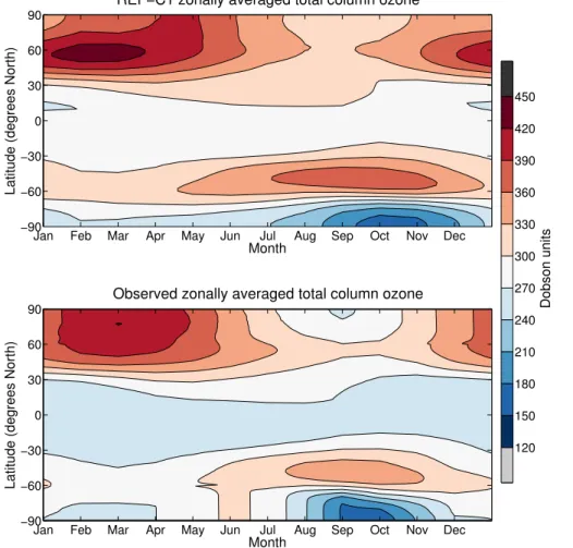
Figure 1 shows zonally averaged TCO over the 2001–2010 period for the REF-C1 hind-cast simulation compared to observations from the Bodeker Scientific TCO database. The yearly zonal structure of TCO compares well to observations. However, there is consistently more ozone almost globally within the REF-C1 simulation. The onset of 10
springtime Antarctic ozone depletion occurs a little later in the REF-C1 simulation com-pared to the observations. This is accompanied by the maximum in ozone depletion occurring later and the persistence of ozone depletion continuing later in the year for the simulation. Despite these temporal differences, the simulated amount of ozone de-stroyed during the ozone hole period is similar to what is observed.
15
4.2 Historical time series
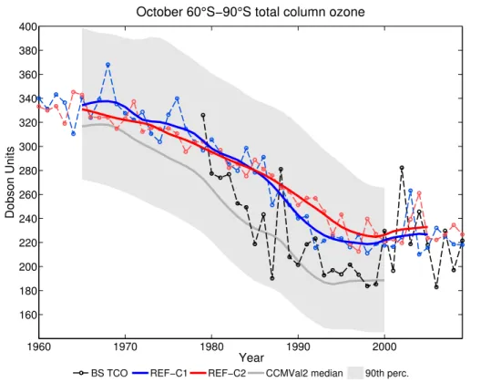
Figure 2 compares observations and the CCMVal-2 ensemble with C1 and REF-C2 simulations of Antarctic TCO averaged between 60–90◦S for October. The latitude range of 60–90◦S was chosen for the ozone comparison, as this area experiences the most significant springtime ozone depletion. The REF-C1 and REF-C2 simulations are 20
consistently producing larger TCOs over the entire historical period examined com-pared to observations and the CCMVal-2 ensemble. However, the C1 and REF-C2 simulations consistently lay inside the CCMVal-2 10th and 90th percentile, and the total amount of ozone depletion from 1960 to 2010 is similar. The inter-annual vari-ability simulated by the model is not as large as in the observations. There are also 25
pe-ACPD
15, 19161–19196, 2015ACCESS-CCM evaluation
K. A. Stone et al.
Title Page
Abstract Introduction
Conclusions References
Tables Figures
◭ ◮
◭ ◮
Back Close
Full Screen / Esc
Printer-friendly Version Interactive Discussion
Discussion
P
a
per
|
Discussion
P
a
per
|
Discussion
P
a
per
|
Discussion
P
a
per
|
riod. This can be attributed to the different SST and SIC datasets used, marking the only difference between the REF-C1 and the historical part of the REF-C2 simulation before 2005.
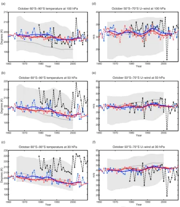
Figure 3 similarly compares the REF-C1 and REF-C2 60–90◦S averaged October temperature and 50–70◦S average zonal winds to ERA-Interim and the CCMVal-2 en-5
semble for the stratospheric pressure levels: 100, 50 and 30 hPa. The latitude range between 50–70◦S was chosen to examine the strong westerlies forming the polar vor-tex boundary.
At 100 hPa the REF-C1 and REF-C2 temperature simulations compare well to the ERA-Interim data, in contrast to the CCMVal-2 ensemble median, which shows a sub-10
stantial cold bias of up to 6 K. The CCMVal-2 ensemble median captures a trend of decreasing temperature; consistent with colder stratospheric temperatures expected to accompany historical ozone depletion. This decreasing temperature is also seen in the C1 and C2 simulations, albeit to a lesser scale. The C1 and REF-C2 zonal wind simulations at 100 hPa compare well with both ERA-Interim and the 15
CCMVal-2 ensemble, with only slightly weaker zonal winds present in CCMVal-2 and the REF-C1 and REF-C2 simulations. This is surprising, as the cold bias present in the 100 hPa CCMVal-2 temperature is expected to be associated with more intense zonal wind. However, these inconsistencies are most likely due to similar temperature gradients between the poles and mid-latitudes seen in both ACCESS-CCM and the 20
CCMVal-2 ensemble. The amount of variation in the REF-C1 and REF-C2 simulations is also similar to what is seen in the ERA-Interim data, and the ERA-Interim data lay entirely within the CCMVal-2 10th and 90th percentiles.
At 50 hPa a significant cold bias exists of around 5 K in the REF-C1 and REF-C2 model runs compared to ERA-Interim data. This is not as pronounced as the CCMVal-25
ACPD
15, 19161–19196, 2015ACCESS-CCM evaluation
K. A. Stone et al.
Title Page
Abstract Introduction
Conclusions References
Tables Figures
◭ ◮
◭ ◮
Back Close
Full Screen / Esc
Printer-friendly Version Interactive Discussion
Discussion
P
a
per
|
Discussion
P
a
per
|
Discussion
P
a
per
|
Discussion
P
a
per
|
the larger ozone concentration present in the ACCESS-CCM model compared to the CCMVal-2 ensemble, as a higher ozone concentration warms the stratosphere through more absorption of UV radiation. A slight decreasing temperature trend is simulated over the historical period, which is not as pronounced as in the CCMVal-2 ensemble. At 50 hPa there is an intensification of the polar vortex due to colder 50 hPa tempera-5
tures in the CCMVal-2 ensemble, however, the REF-C1 and REF-C2 simulations still agree well with ERA-Interim values. The differences between the CCMVal-2 ensemble median and the REF-C1 and REF-C2 simulations increase with time, reaching a max-imum of 5 ms−1at year 2000, and are reflective of the temperature differences.
At 30 hPa, the REF-C1 and REF-C2 simulations of temperature follow the CCMVal-2 10
ensemble median closely, with a large cold temperature bias relative to ERA-Interim, of 10–15 K. However, again the ERA-Interim mostly lay within CCMVal-2 inter-model vari-ability (10th and 90th percentiles). This cold bias is accompanied by slightly stronger zonal winds in the REF-C1 and REF-C2 simulations compared to ERA-Interim. An even stronger zonal wind is associated with the CCMVal-2 ensemble, with a maximum diff er-15
ence of 5 ms−1. The increasing trend in the polar vortex strength seen in the CCMVal-2 models is not as pronounced in the REF-C1 and REF-C2 simulations.
4.3 Ozone, temperature and ClO profiles
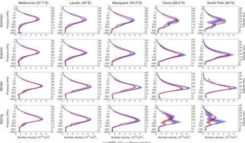
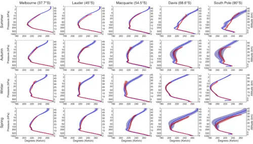
Figure 4 shows vertical ozone profiles seasonally averaged over 2001–2010 for the REF-C1 simulation compared to ozonesonde observations averaged over 2003–2012 20
for five Southern Hemisphere sites and their nearest coincident model grid box. Sim-ilarly, Fig. 5 shows vertical temperature profiles averaged over the same time period and locations. To highlight the variability, shaded regions show one standard devia-tion of the monthly averaged model output for the REF-C1 profiles and one standard deviation divided by√8 for the ozonesonde profiles. The ozonesonde standard devia-25
ACPD
15, 19161–19196, 2015ACCESS-CCM evaluation
K. A. Stone et al.
Title Page
Abstract Introduction
Conclusions References
Tables Figures
◭ ◮
◭ ◮
Back Close
Full Screen / Esc
Printer-friendly Version Interactive Discussion
Discussion
P
a
per
|
Discussion
P
a
per
|
Discussion
P
a
per
|
Discussion
P
a
per
|
between the two datasets for both ozone concentration and temperature are provided in Table 1. Anomalies are visibly present in the upper levels of ozonesonde measure-ments, particularly in the temperature profiles. At these levels measurement sample size is severely reduced, resulting in possible skewed seasonal averages.
Figures 4 and 5 illustrate that there is general agreement in both ozone and tem-5
perature profiles between the ozonesondes and the REF-C1 simulation for Melbourne. The location of the peak in ozone concentration is consistent between REF-C1 and ozonesondes throughout summer, autumn and winter. There is a slight difference dur-ing sprdur-ing, with the model simulatdur-ing a slightly higher ozone peak altitude relative to ozonesondes. Consistently the model simulates excessive ozone peak concentrations 10
between 20 and 25 km, as shown in Table 1. This is largest for autumn, with an ex-cess of 8 % simulated by the model. The REF-C1 temperature profiles agree well with ozonesondes below 100 hPa. However, above 100 hPa there are consistent cold biases of up to 3.1 K that extend up to 10 hPa during all seasons.
The comparison at Lauder and Macquarie Island illustrates poorer agreement be-15
tween the REF-C1 simulation and ozonesonde ozone observations. The ozone con-centration peak altitudes are still consistent between the datasets, with the largest exception at Macquarie during summer, where the REF-C1 profile peak is situated slightly higher. Again, the model is predicting excess ozone concentration peaks dur-ing all seasons, with the largest at Lauder of 13.4 % durdur-ing summer, and at Macquarie 20
of 20.1 % seem during winter. The REF-C1 temperature profiles generally agree well with ozonesondes. However, there is still a cold bias present above 100 hPa, up to 4.5 K seen during summer at Lauder, and 5.6 K at Macquarie near the tropopause at 170 hPa.
Davis (located within the polar vortex collar region) comparisons of REF-C1 and 25
win-ACPD
15, 19161–19196, 2015ACCESS-CCM evaluation
K. A. Stone et al.
Title Page
Abstract Introduction
Conclusions References
Tables Figures
◭ ◮
◭ ◮
Back Close
Full Screen / Esc
Printer-friendly Version Interactive Discussion
Discussion
P
a
per
|
Discussion
P
a
per
|
Discussion
P
a
per
|
Discussion
P
a
per
|
ter. Simulated summer and to a lesser extent, autumn, temperature profiles also show a cold temperature bias, most noticeable between 250 and 30 hPa of up to 6.1 K. The winter simulated temperature profile agrees very well with ozonesondes, in contrast to ozone concentrations, where there is a very large difference. Davis is located in an area that experiences perturbed springtime polar ozone depletion. Here, ozone depletion is 5
captured in the simulated ozone profiles mostly between 50 and 20 hPa. This is in con-trast to what is observed by ozonesonde profiles, where the majority of ozone depletion is seen at a lower altitude, below 50 hPa and centered around 100 hPa. This indicates a clear inadequacy of the model in capturing the springtime vertical ozone structure. The simulated temperature profiles at Davis also show a large cold bias above 70 hPa 10
of up to 13.4 K, associated with the altitude of ozone depletion in the model. The vari-ability, seen in the standard deviations is also much larger during spring for ozoneson-des and REF-C1 compared to other seasons. This is due to the variable nature of springtime Antarctic ozone depletion, and the location of Davis, which is often in the collar region of the polar vortex.
15
Due to the dynamical variability experienced by Davis, with Davis being in the polar vortex edge region, comparisons of simulated and ozonesonde vertical ozone concen-tration and temperature for the South Pole were conducted. The South Pole shows very similar differences between ozonesondes and REF-C1 model simulations for both ozone concentrations and temperature to Davis. Therefore the disparity in the vertical 20
location of springtime ozone depletion seen at Davis is not due to its potential location on the edge of the polar vortex. However, there are some differences. The amount of ozone depletion simulated during spring in the model is now enhanced greatly, with almost all ozone destroyed above 50 hPa. While ozonesondes only show slightly more ozone depletion. The discrepancy in the altitude of significant ozone depletion is still 25
ACPD
15, 19161–19196, 2015ACCESS-CCM evaluation
K. A. Stone et al.
Title Page
Abstract Introduction
Conclusions References
Tables Figures
◭ ◮
◭ ◮
Back Close
Full Screen / Esc
Printer-friendly Version Interactive Discussion
Discussion
P
a
per
|
Discussion
P
a
per
|
Discussion
P
a
per
|
Discussion
P
a
per
|
A consistent ozone excess at all stations during seasons that are not perturbed by springtime ozone loss is seen in the vertical ozone profiles, increasing with increasing latitude (Fig. 4). This suggests possible problems with transport in the model. Also, as the model shows excess ozone globally, cold biases above 10 hPa may also be aff ect-ing gas phase ozone chemical cycles. On a global average scale, the stratospheric cold 5
biases simulated by the model are likely due to incorrect concentrations and distribu-tions of radiatively active gas or problems with the radiative scheme (SPARC-CCMVal, 2010). The two main radiative gases that are tied into the chemistry scheme in the stratosphere are ozone and water vapour. Global water vapour distributions of a pre-vious iteration of this model where analysed in Morgenstern et al. (2009) and where 10
shown to agree well with ERA-40 climatology.
The large differences seen in the vertical structure of perturbed springtime ozone between the REF-C1 simulation and ozonesondes is either chemical or dynamical in nature, or some combination of both. The slightly colder winter temperatures seen in the model over Antarctic regions can have implications for PSC formation and are 15
likely a result of less pole-ward heat transport, analysed through comparison of 45– 75◦S heat flux with MERRA reanalysis (not shown). To investigate the links between the chemistry and dynamics of the problem, Fig. 6 shows a comparison of ClO volume mixing ratio, extracted for the zonal region of 67–70◦S corresponding to Davis and temporally averaged between 2001–2010 for the REF-C1 simulation and 2005–2014 20
for MLS satellite observations. The altitude of large ClO volume mixing ratios is an indi-cation of the altitude of where chemical cycles that are responsible for the destruction of ozone are occurring. ClO has a strong diurnal cycle, with concentrations peaking during sunlit hours. This may cause some disparity between the amount of ClO ob-served by the MLS instrument and simulated by the model. The MLS instrument only 25
ACPD
15, 19161–19196, 2015ACCESS-CCM evaluation
K. A. Stone et al.
Title Page
Abstract Introduction
Conclusions References
Tables Figures
◭ ◮
◭ ◮
Back Close
Full Screen / Esc
Printer-friendly Version Interactive Discussion
Discussion
P
a
per
|
Discussion
P
a
per
|
Discussion
P
a
per
|
Discussion
P
a
per
|
the monthly average model data used. However, while this type of comparison does not allow direct quantitative evaluation of the modelled ClO volume mixing ratios, it can give an indication of the vertical locations of the ClO volume mixing ratio peaks. This provides an indication of where the ozone loss chemical reactions are taking place.
During summer, the structure and peak of the simulated ClO profiles agrees well with 5
MLS measurements. During autumn the model simulates a peak in ClO volume mixing ratio at around 20 hPa that is not captured by the observations. This is most likely due to stratospheric cold bias seen in the model causing late autumn polar stratospheric cloud formation. The winter profiles show very good agreement of the ClO peak location below 20 hPa. However, above 20 hPa there are large differences, with the ClO decline 10
and minimum seen in the MLS measurements at 10 hPa being slightly lower in altitude and much less noticeable in the model. The peak in modelled ClO due to gas phase chemistry at higher altitudes is also slightly lower in the REF-C1 simulation compared to MLS observations. The large differences seen in the volume mixing ratios during winter can be attributed to the inability of the MLS instrument capturing the diurnal cycle at 15
these latitudes. There is a large difference between the REF-C1 simulated ClO and that observed by MLS during spring. At 50 hPa and below, the MLS observed peak in ClO is not captured by the REF-C1 simulations. Above 50 hPa, the REF-C1 simulated ClO peak is also a little lower in altitude compared to MLS, similar to what is seen in winter. These ClO observations are consistent with the vertical structure of springtime 20
ozone concentrations, and that the altitude of ozone depletion is misrepresented by our model over Davis and the South Pole.
These results suggest the colder Antarctic stratospheric temperatures above 100 hPa seen in the model are causing enhanced PSC formation at higher altitudes, and thus more heterogeneous reactions on the surface of PSCs. This is indeed the 25
ACPD
15, 19161–19196, 2015ACCESS-CCM evaluation
K. A. Stone et al.
Title Page
Abstract Introduction
Conclusions References
Tables Figures
◭ ◮
◭ ◮
Back Close
Full Screen / Esc
Printer-friendly Version Interactive Discussion
Discussion
P
a
per
|
Discussion
P
a
per
|
Discussion
P
a
per
|
Discussion
P
a
per
|
further highlighted by the disparity in MLS measured and modelled ClO springtime profiles, with MLS showing a peak due to heterogeneous reactions on PSCs at 50 hPa and below that is not captured well by the model. There is also absence of a defined minimum in the modelled ClO profile seen around 20 hPa in MLS measurements. This agrees well with the large differences seen in the vertical location of ozone depletion 5
simulated for at Davis and the South Pole, consistent with the large springtime cold biases present in the model at 50 and 30 hPa. The lack of ozone depletion at lower altitudes compared to ozonesondes could possible be explained by the lack of STS simulated by the model due to their higher effectiveness at lower altitudes (Solomon, 1999).
10
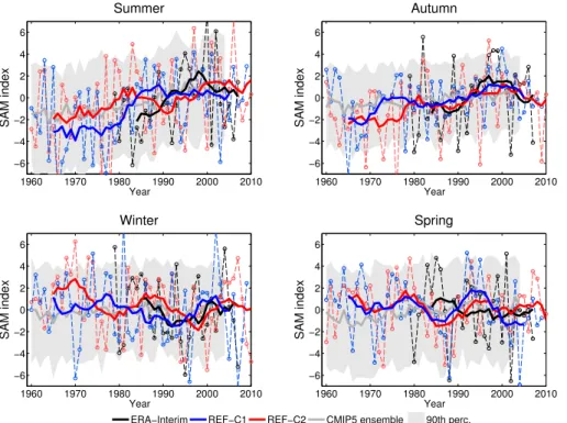
4.4 Southern annular mode
Figure 7 shows Southern Hemisphere seasonal SAM indices for REF-C1 and the his-torical part of REF-C2 compared to ERA-Interim data from 1979–2010 and the recent past section of the historical simulations from CMIP5 runs that used prescribed ozone (Eyring et al., 2013a). The seasonal SAM index was calculated following Morgenstern 15
et al. (2014), using the seasonally averaged difference in area-averaged surface pres-sure between 38.75–61.25◦S and 63.75–90◦S. To be able to appropriately compare to ERA-Interim and CMIP5 data, this value was normalised by subtracting the 1979–2005 mean of the calculated SAM indices. The REF-C1, REF-C2 and ERA-Interim seasonal SAM indices are shown as both the yearly seasonal average (highlighting the year-to-20
year variability) and also as a ten-year running mean (highlighting the comparison to the CMIP5 ensemble). The CMIP5 time series shows the ensemble median and the 10th and 90th percentiles interval of the ensemble range.
During summer the CMIP5 ensemble captures a noticeable increase in the SAM in-dex between 1960–2005, consistent with historical Antarctic ozone depletion. A large 25
year-ACPD
15, 19161–19196, 2015ACCESS-CCM evaluation
K. A. Stone et al.
Title Page
Abstract Introduction
Conclusions References
Tables Figures
◭ ◮
◭ ◮
Back Close
Full Screen / Esc
Printer-friendly Version Interactive Discussion
Discussion
P
a
per
|
Discussion
P
a
per
|
Discussion
P
a
per
|
Discussion
P
a
per
|
to-year variability in the REF-C1 and REF-C2 time-series, which mostly lay within the CMIP5 10th and 90th percentiles and very similar to what is seen in the ERA-Interim data. There are also noticeable differences between the REF-C1 and REF-C2 data, mostly before 1985. This can be mostly attributed to different SSTs and the SICs used between the two model runs, or random climate fluctuations. The differences 5
in temporal Antarctic stratospheric ozone depletion between the REF-C1 and REF-C2 would also be an important influence. The increasing SAM index is representative of a southward shift of the westerly winds and precipitation regimes, and is attributed to both decreasing Antarctic stratospheric ozone concentrations and increasing GHGs. An increasing summer SAM index simulated by the model not only agrees with CMIP5 10
data and ERA-Interim re-analysis, it also complements conclusions from Keeble et al. (2014), which show significant increases in SAM attributed to lower stratospheric ozone depletion within a similar model environment.
Autumn also shows an increase in the SAM index in the CMIP5 ensemble, albeit on a smaller scale to that seen in summer. The REF-C1 and REF-C2 time-series agree 15
well with the CMIP5 data and especially well with the ERA-Interim data. An increase in the SAM index over time is consistent with the CMIP5 ensemble, and the year-to-year variability of the REF-C1 time-series is consistently within the CMIP5 10th and 90th percentiles. However, the REF-C2 seasonal variation shows a frequent low SAM index values outside of the CMIP5 variability, most frequently before 1980. The cause of the 20
positive SAM trend observed during autumn is currently not well understood (Canziani et al., 2014). The seasonal variation seen in the REF-C1 and REF-C2 time-series is also similar to that seen in the ERA-Interim data. The differences between the REF-C1 and REF-C2 time-series are much less pronounced, especially after 1980 where they follow each other closely. The differences before 1980 can be attributed to the 25
different SSTs and SICs used or random climate fluctuations, and less likely due to the differences in stratospheric ozone.
ACPD
15, 19161–19196, 2015ACCESS-CCM evaluation
K. A. Stone et al.
Title Page
Abstract Introduction
Conclusions References
Tables Figures
◭ ◮
◭ ◮
Back Close
Full Screen / Esc
Printer-friendly Version Interactive Discussion
Discussion
P
a
per
|
Discussion
P
a
per
|
Discussion
P
a
per
|
Discussion
P
a
per
|
with the REF-C1 and REF-C2 time series agreeing well. The largest excursion from the CMIP5 ensemble median is seen in the REF-C2 time-series centered around 1970 during winter, where a positive SAM index is seen consistently over 3 years. A notice-able difference between the REF-C1 and REF-C2 winter and spring SAM indexes is a strong decadal correlation during spring, in contrast to the winter comparison. 5
4.5 Zonal wind anomalies
Figure 8 shows 50 hPa average zonal winds of 1979–1988 minus the 2001–2010 av-erage for REF-C1, REF-C2, and ERA-Interim data for the months of August, October and December. The ten-year averages represent the earliest time available in the ERA-Interim and the latest time available in the historical simulations, while also being able 10
to represent important phases in stratospheric springtime Antarctic ozone depletion, with 1979–1988 representing the onset of ozone depletion while 2001–2010 repre-senting the maximum springtime ozone depletion. The months of August, October and December where chosen to represent different stages of the annually forming ozone hole. The ozone hole typically begins forming in late August, reaching a maximum by 15
the end of October, and closing by mid-December.
August shows some small-scale differences between the REF-C1 and REF-C2 rel-ative to ERA-Interim, most likely caused by differences in decadal variations between the model and observations. October shows some larger differences, with an opposite dipole in the western hemisphere when comparing REF-C1 and REF-C2 with ERA-20
Interim. Again, this can be attributed to decadal differences in the variations, and pos-sible differences in the maximum location in zonal wind, which is more pole-ward in ERA-Interim compared to the model simulations. The December differences are very consistent across the REF-C1, REF-C2, and ERA-Interim data, with increasing zonal wind seen south of 60◦S. This is an indication of the strengthening of the polar vortex 25
ACPD
15, 19161–19196, 2015ACCESS-CCM evaluation
K. A. Stone et al.
Title Page
Abstract Introduction
Conclusions References
Tables Figures
◭ ◮
◭ ◮
Back Close
Full Screen / Esc
Printer-friendly Version Interactive Discussion
Discussion
P
a
per
|
Discussion
P
a
per
|
Discussion
P
a
per
|
Discussion
P
a
per
|
5 Conclusions
The ACCESS-CCM model presented here is able to confidently provide an initial con-tribution from Australia to the international community via the Chemistry-Climate Model Initiative (CCMI). It simulates slightly larger October total column ozone values com-pared to observations and the CCMVal-2 ensemble, however simulates a similar ozone 5
decline over the historical period (1960 to 2010). A cold bias compared to ERA-Interim of up to 5 K at 50 hPa and 10–15 K at 30 hPa is present during October. This is an im-provement from the CCMVal-2 ensemble, which shows colder temperatures compared to ACCESS-CCM at 100 and 50 hPa of up to of 5 and 3 K respectively. Our model simulates polar vortex strength above 100 hPa closer to ERA-Interim compared to the 10
CCMVal-2 ensemble median.
Model-simulated seasonal averaged vertical profiles of ozone and temperature com-pared to Southern Hemisphere ozonesondes show very good agreement in ozone ver-tical distribution, concentration and seasonal variation for Melbourne. However, there is less agreement at higher latitudes sites, with peak ozone concentrations in excess of 15
observed values. The largest difference is seen at Davis during winter, with ACCESS-CCM simulating 26.4% excess. A stratospheric cold bias is also present, mostly above 100 hPa and noticeably over polar latitudes during summer of up to 15.3 K. The majority of springtime ozone depletion at Davis and the South Pole is occurring above 50 hPa in ACCESS-CCM compared to being centered near 100 hPa in ozonesondes. This also 20
induces a significant cold bias in the stratosphere during spring at the altitudes of ozone depletion in the model.
The altitude differences of springtime polar ozone loss can be attributed to diff er-ences in simulated ClO profiles during spring, pointing to a modelling deficiency in simulating heterogeneous chlorine release. The MLS instrument shows a peak in ClO 25
alti-ACPD
15, 19161–19196, 2015ACCESS-CCM evaluation
K. A. Stone et al.
Title Page
Abstract Introduction
Conclusions References
Tables Figures
◭ ◮
◭ ◮
Back Close
Full Screen / Esc
Printer-friendly Version Interactive Discussion
Discussion
P
a
per
|
Discussion
P
a
per
|
Discussion
P
a
per
|
Discussion
P
a
per
|
tudes, and thus providing a mechanism for increased ozone loss at higher altitudes. The deficiency in modelling a large springtime ClO peak at lower altitudes, explains the relatively small simulated ozone loss at these altitudes relative to ozonesonde ob-servations, and could possible be due to the models inability simulating supercooled ternary solution polar stratospheric clouds.
5
The large model-ozonesonde differences in the ozone profiles during summer, au-tumn and winter, seasons outside perturbed polar springtime ozone loss conditions, is consistent with the excess ozone seen in the global total column ozone map (Fig. 1), and time series (Fig. 2). This could possibly be due to too much transport in the model, and cold biases above 10 hPa affecting the gas-phase ozone chemical cycles. The 10
drivers of the cold biases and excessive transport within the ACCESS-CCM are un-clear, however, mid-latitude cold biases are likely influenced by incorrect radiatively active gases such as ozone and water vapour or inaccuracies in the radiation scheme. Whereas lower simulated mid-latitude heat flux is likely a driver of the high latitude cold biases.
15
The SAM index for ACCESS-CCM agrees well with ERA-Interim and CMIP5 ensem-ble. All show an increasing SAM index during summer and to a lesser extent autumn, indicating a southward shift of mid-latitude winds and storm tracks. Zonal wind diff er-ences of 1979–1988 average minus 2001–2010 average at 50 hPa during December show increasing high south latitude wind strength, consistent with the simulated in-20
crease in the SAM during summer.
Future versions of this model will follow the UKCA release candidates, with a major goal of obtaining a fully coupled chemistry-climate-ocean model.
Acknowledgements. This work was supported through funding by the Australian Government’s Australian Antarctic Science Grant Program (FoRCES 4012), the Australian Research
Coun-25
cil’s Centre of Excellence for Climate System Science (CE110001028), the Commonwealth Department of the Environment (grant 2011/16853), and NIWA as part of its New Zealand Government-funded, core research, and by the Marsden Fund Council from Government fund-ing, administered by the Royal Society of New Zealand (grant 12-NIW-006). This research was undertaken with the assistance of resources provided at the NCI National Facility systems at
ACPD
15, 19161–19196, 2015ACCESS-CCM evaluation
K. A. Stone et al.
Title Page
Abstract Introduction
Conclusions References
Tables Figures
◭ ◮
◭ ◮
Back Close
Full Screen / Esc
Printer-friendly Version Interactive Discussion
Discussion
P
a
per
|
Discussion
P
a
per
|
Discussion
P
a
per
|
Discussion
P
a
per
|
the Australian National University through the National Computational Merit Allocation Scheme supported by the Australian Government. The authors wish to thank all past ozonesonde ob-servers. All data used in this paper can be downloaded from the CCMI web portal or obtained
from the lead author. We acknowledge the UK Met Office for use of the MetUM.
References 5
Arblaster, J. M. and Meehl, G. A.: Contributions of external forcings to southern annular mode trends, J. Climate, 19, 2896–2905, doi:10.1175/JCLI3774.1, 2006. 19164
Arblaster, J. M., Meehl, G. A., and Karoly, D. J.: Future climate change in the Southern
Hemi-sphere: competing effects of ozone and greenhouse gases, Geophys. Res. Lett., 38, L02701,
doi:10.1029/2010GL045384, 2011. 19164
10
Archibald, A. T., Levine, J. G., and Abraham, N. L.: Impacts of HOxregeneration and recycling
in the oxidation of isoprene: consequences for the composition of past, present and future atmospheres, Geophys. Res. Lett., 38, L05804, doi:10.1029/2010GL046520, 2011. 19166 Austin, J., Scinocca, J., Plummer, D., Oman, L., Waugh, D., Akiyoshi, H., Bekki, S.,
Braesicke, P., Butchart, N., Chipperfield, M., Cugnet, D., Dameris, M., Dhomse, S., Eyring, V.,
15
Frith, S., Garcia, R. R., Garny, H., Gettelman, A., Hardiman, S. C., Kinnison, D., Lamar-que, J. F., Mancini, E., Marchand, M., Michou, M., Morgenstern, O., Nakamura, T., Paw-son, S., Pitari, G., Pyle, J., Rozanov, E., Shepherd, T. G., Shibata, K., Teyssèdre, H., Wil-son, R. J., and Yamashita, Y.: Decline and recovery of total column ozone using a multimodel time series analysis, J. Geophys. Res., 115, D00M10, doi:10.1029/2010JD013857, 2010.
20
19164
Banerjee, A., Archibald, A. T., Maycock, A. C., Telford, P., Abraham, N. L., Yang, X.,
Braesicke, P., and Pyle, J. A.: Lightning NOx, a key chemistry–climate interaction: impacts of
future climate change and consequences for tropospheric oxidising capacity, Atmos. Chem. Phys., 14, 9871–9881, doi:10.5194/acp-14-9871-2014, 2014. 19166
25
Barnett, J. J., Houghton, J. T., and Pyle, J. A.: The temperature dependence of the ozone concentration near the stratopause, Q.J. Roy. Meteor. Soc., 101, 245–257, doi:10.1002/qj.49710142808, 1975. 19164
Bodeker, G. E., Shiona, H., and Eskes, H.: Indicators of Antarctic ozone depletion, Atmos. Chem. Phys., 5, 2603–2615, doi:10.5194/acp-5-2603-2005, 2005. 19167
ACPD
15, 19161–19196, 2015ACCESS-CCM evaluation
K. A. Stone et al.
Title Page
Abstract Introduction
Conclusions References
Tables Figures
◭ ◮
◭ ◮
Back Close
Full Screen / Esc
Printer-friendly Version Interactive Discussion
Discussion
P
a
per
|
Discussion
P
a
per
|
Discussion
P
a
per
|
Discussion
P
a
per
|
Butchart, N., Scaife, A. A., Bourqui, M., and De Grandpre, J.: Simulations of anthropogenic change in the strength of the Brewer–Dobson circulation, Clim. Dynam., 27, 727–741, doi:10.1007/s00382-006-0162-4, 2006. 19164
Canziani, P. O., O’Neill, A., Schofield, R., Raphael, M., Marshall, G. J., and Redaelli, G.: World
climate research programme special workshop on climatic effects of ozone depletion in the
5
Southern Hemisphere, B. Am. Meteorol. Soc., 95, ES101–ES105, doi:10.1175/BAMS-D-13-00143.1, 2014. 19164, 19178
Dameris, M., Godin-Beekmann, S., Alexander, S., Braesicke, P., Chipperfield, M., de Laat, A. T. J., Orsolini, Y., Rex, M., and Santee, M. L.: Update on Polar ozone: past, present, and future, in: Chapter 3 in Scientific Assessment of Ozone Depletion: 2014, Global
10
Ozone Research and Monitoring Project, Report No. 55, World Meteorological Organization, Geneva, Switzerland, 2014. 19163
Davies, T., Cullen, M., and Malcolm, A. J.: A new dynamical core for the Met Office’s global
and regional modelling of the atmosphere, Q. J. Roy. Meteor. Soc., 131, 1759–1782, doi:10.1256/qj.04.101, 2005. 19166
15
Dee, D. P., Uppala, S. M., Simmons, A. J., Berrisford, P., Poli, P., Kobayashi, S., Andrae, U., Balmaseda, M. A., Balsamo, G., Bauer, P., Bechtold, P., Beljaars, A. C. M., van de Berg, L., Bidlot, J., Bormann, N., Delsol, C., Dragani, R., Fuentes, M., Geer, A. J., Haimberger, L., Healy, S. B., Hersbach, H., Hólm, E. V., Isaksen, L., Kållberg, P., Köhler, M., Matricardi, M., McNally, A. P., Monge-Sanz, B. M., Morcrette, J. J., Park, B. K., Peubey, C., de
Ros-20
nay, P., Tavolato, C., Thépaut, J. N., and Vitart, F.: The ERA-Interim reanalysis: configuration and performance of the data assimilation system, Q. J. Roy. Meteor. Soc., 137, 553–597, doi:10.1002/qj.828, 2011. 19168
Edwards, J. M. and Slingo, A.: Studies with a flexible new radiation code. I: Choos-ing a configuration for a large-scale model , Q. J. Roy. Meteor. Soc., 122, 689–719,
25
doi:10.1002/qj.49712253107, 1996. 19166
Eyring, V., Arblaster, J. M., and Cionni, I.: Long-term ozone changes and associated climate impacts in CMIP5 simulations, J. Geophys. Res., 118, 5029–5060, doi:10.1002/jgrd.50316, 2013a. 19177
Eyring, V., Lamarque, J.-F., Hess, P., Arfeuille, F., Bowman, K., Chipperfiel, M. P., Duncan, B.,
30
ACPD
15, 19161–19196, 2015ACCESS-CCM evaluation
K. A. Stone et al.
Title Page
Abstract Introduction
Conclusions References
Tables Figures
◭ ◮
◭ ◮
Back Close
Full Screen / Esc
Printer-friendly Version Interactive Discussion
Discussion
P
a
per
|
Discussion
P
a
per
|
Discussion
P
a
per
|
Discussion
P
a
per
|
Tegtmeier, S., Thomason, L., Tilmes, S., Vernier, J.-P., Waugh, D., and Young, P. Y.: Overview of IGAC/SPARC Chemistry-Climate Model Initiative (CCMI) community simulations in sup-port of upcoming ozone and climate assessments, SPARC Newsletter, 40, 48–66, 2013b. 19163, 19166
Gillett, N. P. and Thompson, D. W. J.: Simulation of recent Southern Hemisphere climate
5
change, Science, 302, 273–275, doi:10.1126/science.1087440, 2003. 19163
Granier, C., Bessagnet, B., Bond, T., D’Angiola, A., Denier van der Gon, H., Frost, G. J., Heil, A., Kaiser, J. W., Kinne, S., Klimont, Z., Kloster, S., Lamarque, J.-F., Liousse, C., Masui, T., Meleux, F., Mieville, A., Ohara, T., Raut, J.-C., Riahi, K., Schultz, M. G., Smith, S. J., Thomp-son, A., van Aardenne, J., van der Werf, G. R., and van Vuuren, D. P.: Evolution of
anthro-10
pogenic and biomass burning emissions of air pollutants at global and regional scales during the 1980–2010 period, Climatic Change, 109, 163–190, doi:10.1007/s10584-011-0154-1, 2011. 19167
Hewitt, H. T., Copsey, D., Culverwell, I. D., Harris, C. M., Hill, R. S. R., Keen, A. B., McLaren, A. J., and Hunke, E. C.: Design and implementation of the infrastructure of
15
HadGEM3: the next-generation Met Office climate modelling system, Geosci. Model Dev.,
4, 223–253, doi:10.5194/gmd-4-223-2011, 2011. 19165
Jones, C. D., Hughes, J. K., Bellouin, N., Hardiman, S. C., Jones, G. S., Knight, J., Lid-dicoat, S., O’Connor, F. M., Andres, R. J., Bell, C., Boo, K.-O., Bozzo, A., Butchart, N., Cadule, P., Corbin, K. D., Doutriaux-Boucher, M., Friedlingstein, P., Gornall, J., Gray, L.,
20
Halloran, P. R., Hurtt, G., Ingram, W. J., Lamarque, J.-F., Law, R. M., Meinshausen, M., Osprey, S., Palin, E. J., Parsons Chini, L., Raddatz, T., Sanderson, M. G., Sellar, A. A., Schurer, A., Valdes, P., Wood, N., Woodward, S., Yoshioka, M., and Zerroukat, M.: The HadGEM2-ES implementation of CMIP5 centennial simulations, Geosci. Model Dev., 4, 543– 570, doi:10.5194/gmd-4-543-2011, 2011. 19167
25
Jonsson, A. I., De Grandpre, J., and Fomichev, V. I.: Doubled CO2-induced cooling in the middle
atmosphere: photochemical analysis of the ozone radiative feedback, J. Geophys. Res., 109, D24103, doi:10.1029/2004JD005093, 2004. 19164
Keeble, J., Braesicke, P., Abraham, N. L., Roscoe, H. K., and Pyle, J. A.: The impact of po-lar stratospheric ozone loss on Southern Hemisphere stratospheric circulation and climate,
30
ACPD
15, 19161–19196, 2015ACCESS-CCM evaluation
K. A. Stone et al.
Title Page
Abstract Introduction
Conclusions References
Tables Figures
◭ ◮
◭ ◮
Back Close
Full Screen / Esc
Printer-friendly Version Interactive Discussion
Discussion
P
a
per
|
Discussion
P
a
per
|
Discussion
P
a
per
|
Discussion
P
a
per
|
Lamarque, J. F., Kyle, G. P., Meinshausen, M., and Riahi, K.: Global and regional evolution of short-lived radiatively-active gases and aerosols in the Representative Concentration Path-ways, Climatic Change, 109, 191–212, doi:10.1007/s10584-011-0155-0, 2011. 19167 Lamarque, J.-F., Shindell, D. T., Josse, B., Young, P. J., Cionni, I., Eyring, V., Bergmann, D.,
Cameron-Smith, P., Collins, W. J., Doherty, R., Dalsoren, S., Faluvegi, G., Folberth, G.,
5
Ghan, S. J., Horowitz, L. W., Lee, Y. H., MacKenzie, I. A., Nagashima, T., Naik, V., Plum-mer, D., Righi, M., Rumbold, S. T., Schulz, M., Skeie, R. B., Stevenson, D. S., Strode, S., Sudo, K., Szopa, S., Voulgarakis, A., and Zeng, G.: The Atmospheric Chemistry and Cli-mate Model Intercomparison Project (ACCMIP): overview and description of models, sim-ulations and climate diagnostics, Geosci. Model Dev., 6, 179–206,
doi:10.5194/gmd-6-179-10
2013, 2013. 19165
Li, F., Stolarski, R. S., and Newman, P. A.: Stratospheric ozone in the post-CFC era, Atmos. Chem. Phys., 9, 2207–2213, doi:10.5194/acp-9-2207-2009, 2009. 19164
Livesey, N. J., Read, W. G., Froidevaux, L., Lambert, A., Manney, G. L., Pumphrey, H. C., Santee, M. L., Schwartz, M. J., Wang, S., and Cofield, R. E.: Version 3.3 Level 2 data
qual-15
ity and description document, Jet Propulsion Laboratory, California Institute of Technology, Pasadena, California, D-33509, 2011. 19169
Meinshausen, M., Smith, S. J., Calvin, K., Daniel, J. S., Kainuma, M. L. T., Lamarque, J. F., Matsumoto, K., Montzka, S. A., Raper, S. C. B., Riahi, K., Thomson, A., Velders, G. J. M., and Vuuren, D. P. P.: The RCP greenhouse gas concentrations and their extensions from 1765 to
20
2300, Climatic Change, 109, 213–241, doi:10.1007/s10584-011-0156-z, 2011. 19166 Morgenstern, O., Braesicke, P., O’Connor, F. M., Bushell, A. C., Johnson, C. E., Osprey, S. M.,
and Pyle, J. A.: Evaluation of the new UKCA climate-composition model – Part 1: The strato-sphere, Geosci. Model Dev., 2, 43–57, doi:10.5194/gmd-2-43-2009, 2009. 19165, 19166, 19175
25
Morgenstern, O., Zeng, G., Luke Abraham, N., Telford, P. J., Braesicke, P., Pyle, J. A., Hardi-man, S. C., O’Connor, F. M., and Johnson, C. E.: Impacts of climate change, ozone recovery, and increasing methane on surface ozone and the tropospheric oxidizing capacity, J. Geo-phys. Res.-Atmos., 118, 1028–1041, doi:10.1029/2012JD018382, 2013. 19165
Morgenstern, O., Zeng, G., and Dean, S. M.: Direct and ozone-mediated forcing of the
30
ACPD
15, 19161–19196, 2015ACCESS-CCM evaluation
K. A. Stone et al.
Title Page
Abstract Introduction
Conclusions References
Tables Figures
◭ ◮
◭ ◮
Back Close
Full Screen / Esc
Printer-friendly Version Interactive Discussion
Discussion
P
a
per
|
Discussion
P
a
per
|
Discussion
P
a
per
|
Discussion
P
a
per
|
Neu, J. L., Prather, M. J., and Penner, J. E.: Global atmospheric chemistry: integrating over fractional cloud cover, J. Geophys. Res., 112, D11306, doi:10.1029/2006JD008007, 2007. 19166
O’Connor, F. M., Johnson, C. E., Morgenstern, O., Abraham, N. L., Braesicke, P., Dalvi, M., Folberth, G. A., Sanderson, M. G., Telford, P. J., Voulgarakis, A., Young, P. J., Zeng, G.,
5
Collins, W. J., and Pyle, J. A.: Evaluation of the new UKCA climate-composition model – Part 2: The Troposphere, Geosci. Model Dev., 7, 41–91, doi:10.5194/gmd-7-41-2014, 2014. 19165
Priestley, A.: A quasi-conservative version of the semi-Lagrangian advection scheme, Mon. Weather Rev., 121, 621–629, doi:10.1175/1520-0493(1993)121<0621:AQCVOT>2.0.CO;2,
10
1993. 19166
Rayner, N. A., Parker, D. E., and Horton, E. B.: Global analyses of sea surface temperature, sea ice, and night marine air temperature since the late nineteenth century, J. Geophys. Res., 108, 4407, doi:10.1029/2002JD002670, 2003. 19166
Riahi, K., Rao, S., Krey, V., Cho, C., Chirkov, V., Fischer, G., Kindermann, G., Nakicenovic, N.,
15
and Rafaj, P.: RCP 8.5 – a scenario of comparatively high greenhouse gas emissions, Cli-matic Change, 109, 33–57, doi:10.1007/s10584-011-0149-y, 2011. 19166
Santee, M. L., Lambert, A., and Read, W. G.: Validation of the Aura Microwave Limb Sounder ClO measurements, J. Geophys. Res., 113, D15S22, doi:10.1029/2007JD008762, 2008. 19169
20
Scaife, A. A., Butchart, N., Warner, C. D., and Swinbank, R.: Impact of a spectral gravity wave
parameterization on the stratosphere in the met office unified model, J. Atmos. Sci., 59,
1473–1489, doi:10.1175/1520-0469(2002)059<1473:IOASGW>2.0.CO;2, 2002. 19166 Schultz, M. G., Heil, A., and Hoelzemann, J. J.: Global wildland fire emissions from 1960 to
2000, Global Biogeochem. Cy., 22, GB2002, doi:10.1029/2007GB003031, 2008. 19167
25
Shepherd, T. G.: Dynamics, stratospheric ozone, and climate change, Atmos. Ocean, 46, 117– 138, doi:10.3137/ao.460106, 2008. 19164
Shindell, D. T. and Schmidt, G. A.: Southern Hemisphere climate response to ozone changes and greenhouse gas increases, Geophy. Res. Lett., 31, L18209, doi:10.1029/2004GL020724, 2004. 19163
30
ACPD
15, 19161–19196, 2015ACCESS-CCM evaluation
K. A. Stone et al.
Title Page
Abstract Introduction
Conclusions References
Tables Figures
◭ ◮
◭ ◮
Back Close
Full Screen / Esc
Printer-friendly Version Interactive Discussion
Discussion
P
a
per
|
Discussion
P
a
per
|
Discussion
P
a
per
|
Discussion
P
a
per
|
SPARC-CCMVal: SPARC CCMVal report on the evaluation of chemistry-climate models, SPARC Report No. 5, WCRP-132, WMO/TD-No. 152, 2010. 19165, 19167, 19175
Taylor, K. E., Stouffer, R. J., and Meehl, G. A.: An overview of CMIP5 and the experiment design,
B. Am. Meteorol. Soc., 93, 485–498, doi:10.1175/BAMS-D-11-00094.1, 2012. 19168 Telford, P. J., Abraham, N. L., Archibald, A. T., Braesicke, P., Dalvi, M., Morgenstern, O.,
5
O’Connor, F. M., Richards, N. A. D., and Pyle, J. A.: Implementation of the Fast-JX Photoly-sis scheme (v6.4) into the UKCA component of the MetUM chemistry-climate model (v7.3), Geosci. Model Dev., 6, 161–177, doi:10.5194/gmd-6-161-2013, 2013. 19166
Thompson, D. W. J., Solomon, S., Kushner, P. J., England, M. H., Grise, K. M., and Karoly, D. J.: Signatures of the Antarctic ozone hole in Southern Hemisphere surface climate change, Nat.
10
Geosci., 4, 741–749, doi:10.1038/ngeo1296, 2011. 19164
van der Werf, G. R., Randerson, J. T., Giglio, L., Collatz, G. J., Kasibhatla, P. S., and Arel-lano Jr., A. F.: Interannual variability in global biomass burning emissions from 1997 to 2004, Atmos. Chem. Phys., 6, 3423–3441, doi:10.5194/acp-6-3423-2006, 2006. 19167
Webster, S., Brown, A. R., and Cameron, D. R.: Improvements to the representation of
15
orography in the Met Office Unified Model, Q. J. Roy. Meteor. Soc., 129, 1989–2010,
doi:10.1256/qj.02.133, 2003. 19166
World Meteorlogical Organization (WMO): Scientific Assessment of Ozone Depletion: 2010, Global Ozone Research and Monitoring Project, Report No. 52, Geneva, Switzerland, 516 pp., 2011. 19164, 19167
20
ACPD
15, 19161–19196, 2015ACCESS-CCM evaluation
K. A. Stone et al.
Title Page
Abstract Introduction
Conclusions References
Tables Figures
◭ ◮
◭ ◮
Back Close
Full Screen / Esc
Printer-friendly Version Interactive Discussion
Discussion
P
a
per
|
Discussion
P
a
per
|
Discussion
P
a
per
|
Discussion
P
a
per
|
Table 1.Vertical profile maximum differences.
Station Melbourne Lauder Macquarie Davis South Pole
Summer Ozone (%) 7.3 13.4 8.9 −5.0 −16.5
Temperature (K) 3.1 4.5 2.5 6.6 10.1
Autumn Ozone (%) 8.0 10.8 14.9 14.8 4.0
Temperature (K) 3.1 2.5 2.7 4.1 5.3
Winter Ozone (%) 5.1 10.4 20.1 26.4 17.1
Temperature (K) 3.1 1.3 4.0 0.5 5.3
Spring Ozone (%) 5.7 7.9 9.0 30.4 40.2
ACPD
15, 19161–19196, 2015ACCESS-CCM evaluation
K. A. Stone et al.
Title Page
Abstract Introduction
Conclusions References
Tables Figures
◭ ◮
◭ ◮
Back Close
Full Screen / Esc
Printer-friendly Version Interactive Discussion
Discussion
P
a
per
|
Discussion
P
a
per
|
Discussion
P
a
per
|
Discussion
P
a
per
|
Month
Latitude (degrees North)
REF−C1 zonally averaged total column ozone
Jan Feb Mar Apr May Jun Jul Aug Sep Oct Nov Dec −90
−60 −30 0 30 60 90
Month
Latitude (degrees North)
Observed zonally averaged total column ozone
Jan Feb Mar Apr May Jun Jul Aug Sep Oct Nov Dec −90
−60 −30 0 30 60 90
120 150 180 210 240 270 300 330 360 390 420 450
Dobson units
Figure 1.Zonally 2001–2010 averaged TCO for REF-C1 hindcast simulation compared to
ACPD
15, 19161–19196, 2015ACCESS-CCM evaluation
K. A. Stone et al.
Title Page
Abstract Introduction
Conclusions References
Tables Figures
◭ ◮
◭ ◮
Back Close
Full Screen / Esc
Printer-friendly Version Interactive Discussion
Discussion
P
a
per
|
Discussion
P
a
per
|
Discussion
P
a
per
|
Discussion
P
a
per
|
1960 1970 1980 1990 2000
160 180 200 220 240 260 280 300 320 340 360 380 400
Year
Dobson Units
October 60°S−90°S total column ozone
BS TCO REF−C1 REF−C2 CCMVal2 median 90th perc.
Figure 2.Time series of REF-C1 and REF-C2 TCO averaged between 60–90◦S compared with