www.atmos-chem-phys.net/14/9403/2014/ doi:10.5194/acp-14-9403-2014
© Author(s) 2014. CC Attribution 3.0 License.
Advances in understanding and parameterization of small-scale
physical processes in the marine Arctic climate system: a review
T. Vihma1,2, R. Pirazzini1, I. Fer3, I. A. Renfrew4, J. Sedlar5,6, M. Tjernström5,6, C. Lüpkes7, T. Nygård1, D. Notz8, J. Weiss9, D. Marsan10, B. Cheng1, G. Birnbaum7, S. Gerland11, D. Chechin12, and J. C. Gascard13
1Finnish Meteorological Institute, Helsinki, Finland 2The University Centre in Svalbard, Longyearbyen, Norway 3University of Bergen, Bergen, Norway
4University of East Anglia, Norwich, UK
5Bert Bolin Center for Climate Research, Stockholm, Sweden
6Department of Meteorology, Stockholm University, Stockholm, Sweden
7Alfred-Wegener-Institut Helmholtz-Zentrum für Polar- und Meeresforschung, Bremerhaven, Germany 8Max Planck Institute for Meteorology, Hamburg, Germany
9LGGE, Université de Grenoble, CNRS, Grenoble, France
10ISTerre, Université de Savoie, CNRS, Le Bourget-du-Lac, France 11Norwegian Polar Institute, Tromsø, Norway
12A. M. Obukhov Institute of Atmospheric Physics, Russian Academy of Sciences, Moscow, Russia 13Université Pierre et Marie Curie, Paris, France
Correspondence to: T. Vihma ([email protected])
Received: 13 November 2013 – Published in Atmos. Chem. Phys. Discuss.: 13 December 2013 Revised: 16 July 2014 – Accepted: 21 July 2014 – Published: 10 September 2014
Abstract. The Arctic climate system includes numerous highly interactive small-scale physical processes in the at-mosphere, sea ice, and ocean. During and since the Interna-tional Polar Year 2007–2009, significant advances have been made in understanding these processes. Here, these recent advances are reviewed, synthesized, and discussed. In atmo-spheric physics, the primary advances have been in cloud physics, radiative transfer, mesoscale cyclones, coastal, and fjordic processes as well as in boundary layer processes and surface fluxes. In sea ice and its snow cover, advances have been made in understanding of the surface albedo and its re-lationships with snow properties, the internal structure of sea ice, the heat and salt transfer in ice, the formation of super-imposed ice and snow ice, and the small-scale dynamics of sea ice. For the ocean, significant advances have been related to exchange processes at the ice–ocean interface, diapycnal mixing, double-diffusive convection, tidal currents and diur-nal resonance. Despite this recent progress, some of these small-scale physical processes are still not sufficiently un-derstood: these include wave–turbulence interactions in the
atmosphere and ocean, the exchange of heat and salt at the ice–ocean interface, and the mechanical weakening of sea ice. Many other processes are reasonably well understood as stand-alone processes but the challenge is to understand their interactions with and impacts and feedbacks on other processes. Uncertainty in the parameterization of small-scale processes continues to be among the greatest challenges fac-ing climate modellfac-ing, particularly in high latitudes. Further improvements in parameterization require new year-round field campaigns on the Arctic sea ice, closely combined with satellite remote sensing studies and numerical model experi-ments.
1 Introduction
parameterized in climate or meteorological/oceanographic forecast models, with their current horizontal resolutions typ-ically of the order of 1 to 100 km. These processes include (a) turbulent mixing in the atmosphere and ocean, (b) cloud and aerosol physics, (c) radiative transfer in the atmosphere, snow, ice, and ocean, (d) exchange of momentum, heat, and matter at air–sea, air–snow, air–ice, snow–ice, and ice–water interfaces, (e) small-scale mechanics in sea ice, (f) sea ice growth and melt, (g) formation of snow ice, superimposed ice, and frazil ice, and (h) topographic effects on the atmo-sphere and ocean in coastal and continental shelf regions.
Better understanding and modelling of the Arctic sea ice decline requires comprehensive, synthetic knowledge of small-scale processes in the atmosphere, snow, ice, and ocean. Such knowledge and related modelling capabilities are also prerequisites for a better understanding of the Arctic amplification of climate warming (Serreze and Barry, 2011), for which several processes have been proposed. Among them, the snow/ice albedo feedback has received most atten-tion (e.g. Flanner et al., 2011; Hudson, 2011); in addiatten-tion to its direct effect, it enhances the Arctic amplification by strengthening the water vapour and cloud radiative feedbacks (Graversen and Wang, 2009). Further, feedbacks related to the shape of the temperature profile (Pithan and Mauritsen, 2014), the small heat capacity of the shallow stably strati-fied boundary layer (Esau and Zilitinkevich, 2010) and in-creased autumn–winter energy loss from the ocean (Over-land et al., 2008; Screen and Simmonds, 2010a) tend to am-plify Arctic warming as do the effects of aerosols. It has been suggested that black carbon aerosols reduce the sur-face albedo (e.g. Hadley and Kirchstetter, 2012) and warm the atmosphere (e.g. Quinn et al., 2008), while other aerosols affect the optical properties of the clouds and precipitation processes (e.g. Fridlind et al., 2012; Solomon et al., 2011). In addition to the above-mentioned small-scale processes, an increase in the advection of heat and moisture from lower lat-itudes also contributes to the Arctic amplification (Graversen et al., 2008; Kapsch et al., 2013). The relative importance of the above-mentioned processes in the Arctic is not well un-derstood.
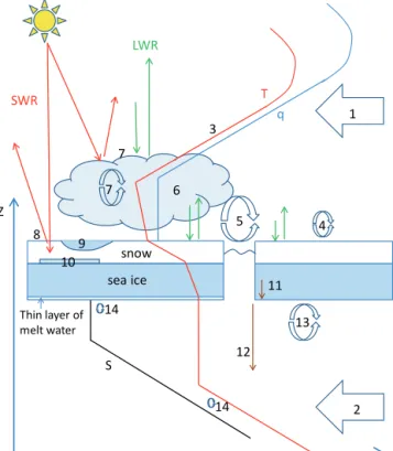
Small-scale processes are most active and important in a layer that starts from the base of the ocean pycnocline and extends up to the top of the boundary layer capping inver-sion in the atmosphere, as schematically illustrated in Fig. 1. This layer extends down 300 m into the ocean (Dmitrenko et al., 2008) and typically up 100–1000 m in the atmosphere (Tjernström and Graversen, 2009), but seasonal and regional variations are large. This layer includes large vertical gradi-ents in temperature, salinity, air humidity, and wind/current speed; these gradients are generated by a complex interac-tion of large-scale circulainterac-tion and small-scale processes. The large gradients are the driving force for turbulent and con-ductive exchange processes in a vertical direction. Further, the layer bounded by the ocean pycnocline and air tempera-ture inversion includes major variations in radiative transfer.
4 snow
sea ice
T q
LWR
SWR
S
Increasing temperature (T), specific humidity (q), and salinity (S) Z
3
2 5
6 7
8 9
1
7
11 10
13
12
14 14
Thin layer of melt water
Figure 1. Simplified presentation of physical processes and verti-cal profiles of temperature (T), air humidity (q), and ocean salinity (S) in the marine Arctic climate system. In reality, the shape of the profiles varies in time and space. The numbers indicate the follow-ing processes: 1 – atmospheric advection of heat and moisture to the Arctic; 2 – oceanic advection of heat and salt to the Arctic; 3 – generation of temperature and humidity inversions; 4 – turbulence in stable boundary layer; 5 – convection over leads and polynyas; 6 – cloud microphysics; 7 – cloud–radiation–turbulence interactions; 8 – reflection and penetration of solar radiation in snow/ice; 9 – sur-face melt and pond formation; 10 – formation of superimposed ice and snow ice; 11 – gravity drainage of salt in sea ice; 12 – brine for-mation; 13 – turbulent exchange of momentum, heat and salt during ice growth; and 14 – double-diffusive convection. More detailed il-lustration of small-scale processes is given in Figs. 2–12.
Compared to a dry atmosphere, the ocean, sea ice, snow, and clouds have a much higher long-wave emissivity and a much lower shortwave transmissivity (Perovich et al., 2007a, b).
except for sea ice dynamics where many important small-scale processes act horizontally.
Processes on different scales are strongly interactive. On one hand, large-scale circulation and related lateral advec-tion of heat and water vapour/freshwater in the atmosphere (Graversen et al., 2011; Sedlar and Devasthale, 2012; Kap-sch et al., 2013) and ocean (Mauldin et al., 2010; Lique and Steele, 2012) strongly affect the boundary conditions for small-scale processes in the Arctic. On the other hand, small-scale processes modify the large-scale circulation via a number of interactive processes. For example, frictional con-vergence in the atmospheric boundary layer (ABL; see Ta-ble A1 for acronyms) affects the evolution of cyclones while brine release from sea ice affects deep convection and ver-tical stratification in the ocean and, hence, the global ther-mohaline circulation. From the point of view of climate and operational modelling, the wide spatial and temporal range of important processes is a major restriction. The important scales range from micrometres (e.g. cloud physics) to thou-sands of kilometres (planetary waves). As models cannot re-solve all scales of motion, many fundamentally important processes need to be parameterized using simplified physics and empirical relationships to resolved grid-scale variables. Variability on the “mesoscale” (approximately 5–500 km in scale) is at the boundary of what is resolved and what must be parameterized in global numerical weather prediction and climate models. In the Arctic, this includes polar mesoscale cyclones, fronts, and orographic flows while there are also a wide range of oceanographic processes at these scales.
In sub-grid-scale parameterizations, the small-scale pro-cesses are presented as functions of those variables that can be resolved by the model grid. Sub-grid-scale parameteri-zation is one of the issues in climate models that are most prone to uncertainties and errors. This is for several reasons: (a) processes are often so complicated that it is not possible to accurately describe them solely on the basis of resolved variables, (b) models have errors in the resolved variables, (c) the resolved variables represent a large volume (grid cell) but there are large variations in the sub-grid-scale processes inside the grid cell, (d) the physics of small-scale processes is often not sufficiently well understood, (e) parameterizations require experimental data to constrain closure assumptions and the amount of such data may not be sufficient (in vol-ume or in range), and (f) parameterizations are often tuned to make the overall performance of models better, according to Steeneveld et al. (2010), even when this makes the descrip-tion of the particular small-scale process worse. The latter is a source of compensating errors and further inhibits model development, since improvements in one particular process via tuning often results in degradation in the overall model performance.
Present-day climate and numerical weather prediction (NWP) models and atmospheric reanalyses include large er-rors in small-scale processes. For example, in a validation of six regional climate models against year-round
observa-tions at the drifting ice station of the Surface Heat Budget of the Arctic Ocean (SHEBA), Tjernström et al. (2005) ob-served that the turbulent heat fluxes were mostly unreliable with insignificant correlations with observed fluxes and an-nual accumulated values an order of magnitude larger than observed. The downward shortwave and long-wave radiation in the six models were systematically biased negative. Tjern-ström et al. (2008) showed that the radiation errors were strongly related to errors in cloud occurrence, heights, and properties (such as water and ice content and their vertical distribution). In an evaluation of the latest atmospheric re-analyses against independent tethersonde sounding data from the central Arctic sea ice, Jakobson et al. (2012) showed that all five reanalyses included in the evaluation had large systematic errors. Even the best one (ERA-Interim of the ECMWF, 2012; Dee et al., 2011) suffered from a warm bias of up to 2◦C in the lowermost 400 m layer and a significant moist bias throughout the lowermost 900 m. The observed bi-ases in temperature, humidity, and wind speed were in many cases comparable to or even larger than the climatological trends during the latest decades. This represents a major chal-lenge for investigations of the recent Arctic warming, which are often based on atmospheric reanalyses. If the errors are solely systematic, then reanalyses may still yield useful in-formation on trends, but for many variables and regions, we lack the observations to determine if the errors are systematic or not.
The above-mentioned evaluation studies have addressed reanalyses and climate models, but little is known about the quality of operational weather forecasts in the central Arctic. Nordeng et al. (2007) reviewed the challenges in the field, and Jung and Leutbecher (2007) evaluated the ECMWF fore-casting system, but quantitative comparisons between oper-ational forecasts and observations taken at ice stations, re-search vessels, and aircraft in the central Arctic have been very limited (Birch et al., 2009). More studies have been car-ried out for the Arctic marginal seas and coastal areas (Hines and Bromwich, 2008, Lammert et al., 2010; Renfrew et al., 2009b). Forecasting of polar lows and other mesoscale cy-clones is discussed in Sect. 2.3.2.
latitudes; the latter is separated from the free atmosphere by the residual layer (Zilitinkevich and Esau, 2005). This makes the Arctic ABL more liable to the effects of propagating in-ternal gravity waves. Also, the common presence of mixed-phase clouds in the Arctic marks a drastic difference from lower latitudes; observations of liquid water present in clouds at temperatures down to−34◦C during SHEBA (Beesley et al., 2000; Intrieri et al., 2002) demonstrated the need to de-velop better parameterization schemes for the ice and liquid water fractions (Gorodetskaya et al., 2008). In the past, fore-cast centres running global climate or NWP models have not paid enough attention to problems in physical parameteriza-tions in the Arctic, but the situation is improving with the Arctic coming more into focus, driven by the worldwide at-tention to Arctic climate change and the increasing need for operational weather and marine forecasting services in the Arctic.
During the International Polar Year 2007–2009 (IPY), a large effort was made for new field observations, data analy-ses, and model experiments addressing small-scale processes in the Arctic atmosphere–sea-ice–ocean system. One of the major efforts was the European project “Developing Arctic Modeling and Observing Capabilities for Long-term Envi-ronmental Studies” (DAMOCLES, in 2005–2009), for which this special issue is dedicated. The project included an exten-sive amount of in situ observations in the Arctic, supported by remote sensing, data analyses, and model experiments. During DAMOCLES, the drifting ice station Tara was a plat-form for oceanographic, sea ice, and meteorological research (Gascard et al., 2008). In addition, oceanographic and sea ice observations were carried out by several ships, meteo-rological research was conducted on ships, including short drift stations, by research aircraft, and at coastal sites. Fur-thermore, drifting buoys, underwater gliders, and moorings collected extensive sets of oceanographic, sea ice, and mete-orological observations. A DAMOCLES synthesis paper on the large-scale state and change of the Arctic climate sys-tem is presented in Döscher et al. (2014), while our focus is on small-scale processes. Small-scale physical processes in the Arctic Ocean were reviewed by Padman (1995), and other reviews on certain aspects on small-scale processes in high latitudes have been published more recently. Bourassa et al. (2013) focused on radiative and turbulent surface fluxes and remote sensing observations, and Heygster et al. (2012) addressed the DAMOCLES advances in sea ice remote sens-ing, which is related to micro-scale processes in snow and ice. Hunke et al. (2011) and Notz (2012) focused on sea ice physics and modelling, and Meier et al. (2014) reviewed the recent changes in Arctic sea ice and their impacts on biology and human activity. Rudels et al. (2013) reviewed the ocean circulation and water mass properties in the Eurasian Basin of the Arctic Ocean.
In this review we focus on the advances in research on small-scale processes in the Arctic since the start of the IPY, addressing physical processes only and defining small-scale
processes as those that need to be parameterized in climate models. Due to the above-mentioned recent papers, we will not address issues related to remote sensing of the ocean sur-face and sea ice. This review is organized in separate sec-tions for small-scale processes in the atmosphere (Sect. 2), sea ice and snow (Sect. 3), and ocean (Sect. 4), with a cross-disciplinary synthesis, discussion, conclusions, and outlook in Sects. 5 and 6. A reader not interested in specifics of all fields can skip some of Sects. 2, 3, or 4.
2 Atmosphere
2.1 Vertical structure and boundary layer processes Many of the small-scale processes in the Arctic atmosphere closely interact with the vertical structure of the atmo-sphere, modifying it and being constrained by it. The ver-tical structure of the Arctic atmosphere is characterized by an ABL capped by temperature and specific humidity inver-sions (hereafter “humidity inverinver-sions”), The inverinver-sions are generated by the combined effects of the negative radiation balance of the sea ice surface, the direct radiative cooling of the air, and the horizontal advection from lower latitudes (Fig. 1). The temperature inversion layer has a strong sta-ble stratification, whereas the ABL stratification is typically stable or near-neutral; the latter stage is most often due to wind shear but, in conditions of large downward radiation, also due to surface heating. Above the ABL, mixed layers can also occur inside and below clouds (Sect. 2.2).
2.1.1 Temperature and humidity inversions
inversions capping a near-neutral ABL, with no intermediary state. In winter, shifts between the two states are rapid, pre-sumably depending on the presence of stratocumulus clouds, in which radiative processes and in-cloud turbulent dynam-ics together cause the shift of the inversion base from the surface to the air (Tjernström and Graversen, 2009). There is also a pronounced annual cycle; in SHEBA, data surface-based inversions were most common in winter and autumn, accounting for roughly 50 % of the cases whereas in sum-mer practically all inversions were elevated ones on top of a near-neutral ABL. Since SHEBA, however, the occurrence of surface-based inversions in autumn has most probably de-creased due to the sea ice decline.
Using the Atmospheric Infrared Sounder data, Devasthale et al. (2010) estimated that the area-averaged (70 to 90◦N) clear-sky temperature inversion frequency is 70–90 % for summer and approximately 90 % for winter. Raddatz et al. (2011) found similar temperature inversion frequencies for a Canadian polynya region, whereas Tjernström and Gra-versen (2009) reported, based on SHEBA, that inversions, ei-ther surface-based or elevated, are practically always present in the central Arctic. The spatial distribution of temperature inversions is inhomogeneous and strongly controlled by the surface type, the prevailing large-scale circulation conditions and by coastal topography (Pavelsky et al., 2011; Wetzel and Brummer, 2011; Kilpeläinen et al., 2012).
The strongest temperature inversions are most often found in the lowermost kilometre whereas the subsequent weaker inversions are nearly randomly distributed in the lowest 3 km (Tjernström and Graversen, 2009). The frequency, depth, and strength of temperature inversions have been found to cor-relate positively with each other, both spatially and tempo-rally, and correlate negatively with surface temperature (Dev-asthale et al., 2010; Zhang et al., 2011). However, the nega-tive correlation between the inversion strength and surface temperature is noticeably weaker in summer (Fig. 2), pre-sumably due to a different formation mechanism: the sum-mer inversion formation is probably dominated by warm air advection from lower latitudes while in winter the inversions are often generated due to radiation loss at the surface (Dev-asthale et al., 2010). Vihma et al. (2011) reported that temper-ature inversions on the coast of Svalbard are strongly affected by the synoptic-scale weather conditions such as 850 hPa geopotential, temperature, and humidity. In addition, during winter temperature inversion strength over the ocean has a negative correlation with sea ice concentration (Pavelsky et al., 2011).
A particular feature in the Arctic atmosphere that rarely, if ever, occurs at lower latitudes is that specific humidity very often increases across the ABL capping inversion, even for cases where the relative humidity in fact drops in the vertical (Tjernström et al., 2004). Importantly, this causes the entrain-ment of free troposphere air into the ABL to be a source of moisture, rather than a sink which is the case practically ev-erywhere else on Earth. This contributes to the very moist
Figure 2. Histograms of inversion strength and surface temperature for summer (left column) and winter (right column) months in the Arctic, based on Atmospheric Infrared Sounder data. Note that the
xandyaxes are different for summer and winter months and inver-sion strength is multiplied by 10. Each temperature–temperature bin is normalized by the total number of observations in the entire his-togram. Reproduced with permission from Devasthale et al. (2010).
al. (2012) include SHEBA and several years of data from Barrow, hence possibly indicating that there may also be re-gional differences. A nonlinear relationship between humid-ity and temperature inversion strength is clearly found in all seasons except during summer (Devasthale et al., 2011).
Temperature and humidity inversions also have no-table implications for the long-wave radiation. Bintanja et al. (2011) and Pithan and Mauritsen (2014) demonstrated that atmospheric near-surface cooling efficiency decreases markedly with temperature inversion strength, as the inver-sion layer damps the infrared cooling to space, and Boé et al. (2009) obtained analogous results for the role of air tem-perature inversion in reducing the radiative cooling of the ocean surface. Humidity inversions, in turn, can contribute up to 50 % of the total amount of condensed water vapour in a relatively dry atmosphere in winter and spring, which can significantly influence the long-wave radiative characteristics of the atmosphere (Devasthale et al., 2011), and they are pre-sumably vital for the formation and maintenance of Arctic clouds (Sect. 2.2.1).
Inversions are a robust metric to evaluate the reproducibil-ity of ABL processes in numerical models (Devasthale et al., 2011). Currently, Arctic temperature and humidity inver-sions are not realistically captured with respect to strength, depth, and base height by operational weather forecasting models (Lammert et al., 2010), climate models (Medeiros et al., 2011), high-resolution mesoscale models (Kilpeläinen et al., 2012), or even reanalyses (Lüpkes et al., 2010; Jakobson et al., 2012; Serreze et al., 2012). In particular, it is the nature of the Arctic atmosphere to contain multiple inversion layers and this is not reproduced in the models (Kilpeläinen et al., 2012). The errors in temperature inversion characteristics are related to deficits in the simulation of stable boundary layer (SBL) turbulence, clouds, radiative transfer, and surface en-ergy budget (Lammert et al., 2010; Kilpeläinen et al., 2012) but are also sensitive to vertical resolution in models.
2.1.2 Stable boundary layer
Over sea ice in the central Arctic, the ABL is typically sta-bly stratified during 6 winter months and is near-neutral or weakly stable during the other months (Persson et al., 2002; Sect. 2.1.1). Although cases of near-neutral stratification oc-cur throughout the year, from the point of view of under-standing and parameterization of the ABL over sea ice, the main challenges are related to stable stratification and this will be our focus here. The inner part of the Arctic Ocean, where the ice concentration is high and the surface is rela-tively flat and homogeneous, is ideal for SBL studies (e.g. Heinemann, 2008). Research on the Arctic SBL is strongly motivated by the major problems that climate models and re-analyses have in stably stratified conditions. Further, there are important feedback mechanisms related to temperature inversion (Sect. 5.3).
A large part of the recent advance in research is still based on analyses of data from the SHEBA experiment. Important issues addressed in recent research include (a) scaling of SBL turbulence and (b) presence of turbulence under very stable stratification. Related to both (a) and (b), one of the main sources of uncertainty in SBL data analyses and modelling is the large scatter between experimental functions that de-scribe the stability-dependent relationships between vertical gradients and fluxes. Until recently, these formulae have not been based on Arctic data, but Grachev et al. (2007a, b) de-rived new formulae for stable stratification on the basis of SHEBA data. Considering (a), the traditional scaling, based on the Monin–Obukhov similarity theory, is such that the flux–gradient relationships depend on the stability parame-terz / L, where the Obukhov lengthLdepends on the turbu-lent fluxes. Mauritsen and Svensson (2007) and Grachev et al. (2012) demonstrated that, for moderately and very stable conditions, a scaling simply based on the vertical gradients (expressed in terms of the gradient Richardson number, Ri) is better, because in such conditions the vertical gradients are large and their errors are relatively small. Further, there is no self-correlation between fluxes andz / L.
Considering (b), on the basis of SHEBA and mid-latitude data, Sorbjan and Grachev (2010) concluded that the neces-sary condition for the presence of continuous turbulence is that Ri < 0.7, which is a much larger value than expected on the basis of older studies. Intermittent turbulence is, how-ever, present in the atmosphere even under very stable strat-ification with Ri≫1. This is related to the anisotropy of turbulence, which allows enhanced horizontal mixing, and to internal waves, which preserve vertical momentum mix-ing (Galperin et al., 2007; Mauritsen and Svensson, 2007). The energy of internal waves is associated with the turbu-lent potential energy (TPE), the importance of which has re-cently been better understood (Mauritsen et al., 2007; Zil-itinkevich et al., 2013), in addition to the well-known impor-tance of the turbulent kinetic energy, TKE. If TPE is taken into account, it follows that there is no critical Ri and tur-bulence can survive in the very stable boundary layer. An-other approach to treat the very stable stratification is based on the quasi-normal-scale elimination (QNSE) theory, which also takes into account waves and the turbulence anisotropy (Sukoriansky et al., 2005). This is enabled by the spectral na-ture of QNSE, based on ensemble averaging over infinitesi-mally thin spectral shells. Implemented in the NWP model HIRLAM, the QNSE approach yielded promising results for the Arctic compared against SHEBA data (Sukoriansky et al., 2005).
lead or polynya
sea ice sea ice
wind
Sen Growth of convective IBL
Growth of stable IBL
sea smoke wind acceleration
form drag due to floe edge
entrainment
enhanced turbulence
Turbulence due to wind shear only
new ice formation Lat
H
b
a
Figure 3. Convection over leads and polynyas: (a) sea smoke originating from leads in the Fram Strait on 7 March 2013 (photo: C. Lüpkes), (b) schematic presentation of ABL processes over a lead/polynya. Sen and Lat are the turbulent fluxes of sensible and latent heat, respectively.
thermal coupling between the snow surface and near-surface air. Also, Sterk et al. (2013) simulated the lowest near-surface temperatures in conditions of non-zero wind speed.
A low-level jet (LLJ) is a distinctive feature of the SBL; it is often generated by inertial oscillations related to the estab-lishment of stable stratification, and it affects the SBL turbu-lence via top-down mixing due to the large wind shear below the jet core. An analytical model for an LLJ was presented by Thorpe and Guymer (1977). Recently, ReVelle and Nils-son (2008) improved the description of frictional effects in such a model and obtained promising results for the Arctic Ocean. New observations of LLJs over the Arctic Ocean in-clude the work of Jakobson et al. (2013) based on tethered soundings at Tara. In their data, baroclinicity related to tran-sient cyclones was the most important forcing mechanism for LLJs. On average, the baroclinic jets were strong and warm, occurring at lower altitudes than other jets, related among others to inertial oscillations and gusts.
Considering ABL modelling, it is well understood that the ABL schemes commonly applied in climate models and NWP yield excessive heat and momentum fluxes in the SBL (Cuxart et al., 2006; Tjernström et al., 2005), typically
re-sulting in a warm bias near the surface (Atlaskin and Vihma, 2012). In the Arctic, Byrkjedal et al. (2007) demonstrated the importance of a high vertical resolution: not surprisingly, model experiments with 90 levels in the vertical yielded much better results than those with 31 levels, the latter be-ing typical for climate models contributbe-ing to the IPCC AR4. The high-resolution simulations significantly reduced the warm bias and the excessive turbulent fluxes of heat and momentum that were present in the coarse resolution results over the Arctic Ocean.
2.1.3 Convection over leads, polynyas, and the open ocean
Although the Arctic ABL has a predominantly stable or near-neutral stratification, convection occurs as well. This is mostly due to the coexistence of ice and open water surfaces causing strong gradients in the surface temperatures. The in-fluence of open water on the atmosphere strongly depends on the season, being largest in winter and smallest in sum-mer (Bromwich et al., 2009; Kay et al., 2011). Convection may appear over leads, polynyas, and over the open ocean during cold air outbreaks. Thus, there is a large variability in the involved spatial scales, and different parameterizations of turbulence are required. Convection over leads and polynyas (Fig. 3) has been studied since the 1970s (e.g. Andreas et al., 1979). As summarized by Lüpkes et al. (2012b) progress has been made during recent decades mainly with respect to the parameterization of energy fluxes at the lead surface. For example, the Andreas and Cash (1999) parameterization states that the transport of sensible heat is more efficient over small leads than over large leads due to the combined ef-fect of forced and free convection. Recently, based on the lead distribution as analysed from a SPOT satellite image, Marcq and Weiss (2012) found that this dependence can in-crease heat fluxes over a large region of the Arctic by up to 55 % since the small leads are dominating. Also, Over-land et al. (2000) (observations) and Lüpkes et al. (2008a) (one-dimensional air–ice modelling) point to the strong po-tential impact of atmospheric convection over leads on the surface energy budget. Both found that the net heat flux over an ice-covered region in the inner Arctic was close to zero due to a balance of downward fluxes during slightly stable near-surface stratification and upward fluxes from leads.
Although the effect of a single lead on the temperature is small, the integral effect of convection over leads can be very large: according to the model simulations by Lüpkes et al. (2008a), during polar night under clear skies, a 1 % de-crease in sea ice concentration results in up to a 3.5 K in-crease of the near-surface air temperature, if the air mass flows over the sea ice long enough (48 h). Polar WRF experi-ments by Bromwich et al. (2009) revealed that in winter over a region with an ice concentration of about 60 %, the grid-averaged surface temperature increased by 14 K compared to an experiment with 100 % ice concentration. For Antarctic winter, Valkonen et al. (2008) obtained a maximum of 13 K sensitivity of the 2 m air temperature to the sea ice concen-tration data set applied (all based on passive microwave ob-servations). A related modelling challenge is the formation of new ice in leads and polynyas (Fig. 3; Sect. 4.1), which strongly affects the surface temperature, the release of la-tent and sensible heat, and further the evolution of the ABL (Tisler et al., 2008). In particular, the modelling of thin ice growth is difficult due to the required resolution, but also the relation between the transfer coefficients of momentum and heat/humidity still requires future work (Fiedler et al., 2010).
The height reached by convective plumes strongly depends on the width of the lead/polynya, wind speed, surface air tem-perature difference, and the background stratification against which the convection has to work (e.g. Liu et al., 2006). On the basis of airborne observations and high-resolution mod-elling, Lüpkes et al. (2008b, 2012b) concluded that convec-tion over 1–2 km wide leads reached altitudes of 50–300 m depending on the boundary layer structure on the upstream side of leads. On the basis of aircraft in situ, drop sonde, and lidar observations, Lampert et al. (2012) observed that over areas with many leads, the potential temperature decreased with height in the lowermost 50 m and then was nearly con-stant due to convective mixing up to the height of 100–200 m. When the leads were frozen and their fraction was small, however, an SBL extended up to a height of 200–300 m.
Ebner et al. (2011) showed in a modelling study that con-vective plumes generated over the Laptev Sea polynya influ-ence atmospheric turbulinflu-ence even 500 km downstream of the polynya, and Hebbinghaus et al. (2006) found that cyclonic vortices can be generated or intensified over polynyas due to convective processes. Such processes over large polynyas may be important with respect to the drastic changes in sea ice cover observed in recent years.
In models, difficulties arise in the treatment of plumes generated over leads, which interact with the stable or near-neutral environment when the convective internal boundary layer is growing (Fig. 3). Only first attempts have been made to account for the nonlocal character of turbulent fluxes in the plume regions at higher ABL levels (Lüpkes et al., 2008b). Processes in the upper ABL need to be investigated in fu-ture also with the help of Large Eddy Simulation (LES). For example, Esau (2007) found that the structure of turbulent regimes over leads can be extremely complicated under light winds as often found in Arctic regions. This finding forms a challenge for future improved parameterizations of energy transport.
on the regional ocean–atmosphere heat flux. Furthermore, strong off-ice winds, typical for CAOs, have a large impact on the drift of sea ice in the marginal ice zone (MIZ), which in turn affects the CAO development. Thus, it is important to investigate small-scale physical processes in CAOs such as ABL turbulence in strong convective regimes as well as cloud physics.
Lüpkes et al. (2012b) determined that the simplest possi-bility for successfully parameterizing turbulent transport in a strong convective regime is to use closures allowing counter-gradient transport of heat. Applying a mesoscale model with different grid sizes, Chechin et al. (2013) found for ideal-ized cases that the strength of the ice breeze developing in CAOs over open water downstream of the MIZ was strongly affected by the grid sizes: models with grid sizes larger than 20 km tend to underestimate the wind speed close to the ice edge. This finding confirms earlier results by Renfrew et al. (2009a, b) and Haine et al. (2009). Since the ice breeze occurring in a region of roughly 100 km width along the po-lar ice edges influences the energy fluxes, there might be a systematic underestimation of surface energy fluxes in large-scale models.
One of the most striking small-scale features during CAOs is the occurrence of roll convection, which has been exten-sively studied in the last decades (Liu et al., 2006). There are, however, still fundamental questions under discussion. Gryschka et al. (2008) found in an LES study that in case of strong surface heating and weak wind shear, surface inhomo-geneity in the MIZ is an important factor for the generation of convection rolls. This finding also stresses the importance of a close-to-reality treatment of the MIZ processes including the near-surface-fluxes (see Sect. 2.1.4).
2.1.4 Surface roughness and momentum flux
The drift speed of Arctic sea ice has increased during re-cent decades (Rampal et al., 2009; Spreen et al., 2011). In-creased wind speeds have contributed to the drift acceleration between 1950 and 2006 (Häkkinen et al., 2008), but not be-tween 1989 and 2009 (Vihma et al., 2012). Instead, the recent increasing trend in drift speeds is mostly due to ice becoming thinner and mechanically weaker (Sect. 3.3.1). To reliably model the ice drift velocity field and ice export out of the Arctic, it is essential to accurately parameterize the transport of momentum from the atmosphere to the sea ice. Moreover, the friction at the surface determines the atmospheric cross-isobaric mass flux, sometimes called Ekman transport, that is very important for the proper simulation of the lifetime of synoptic-scale weather systems.
The momentum flux depends on the wind velocity, ther-mal stratification in the ABL, and aerodynamic roughness of ice/snow surface, which can be expressed as a roughness length (z0) or drag coefficient (CD10N referring to that at 10 m height under neutral stratification). In addition to the skin friction over smooth ice/snow surface, the aerodynamic
roughness of sea ice is affected by factors generating form drag: ridges, floe edges, and sastrugi (Andreas et al., 2010a, b; Andreas, 2011; Lüpkes et al., 2012a, 2013). This generates a challenge for operational modelling: the above-mentioned characteristics of sea ice surface vary rapidly in time and of-ten over small spatial scales, but they are difficult to observe by remote sensing. Over broken sea ice cover, however, the form drag is mostly caused by floe edges, whose occurrence is related to the sea ice concentration, which can be observed by remote sensing.
z0 of sea ice can be calculated on the basis of tower or aircraft observations. However, the results are not directly comparable as tower observations are not necessarily rep-resentative of the wider surroundings where the occurrence of ice ridges, floe edges, and sastrugi may differ from that in the footprint area of the tower. New results for the Arc-tic sea ice, based on the tower observations from SHEBA, include those by Andreas et al. (2010a, b). A significant ad-vance has been the better understanding of the differences betweenz0in winter and summer. For winter conditions, An-dreas et al. (2010a) propose a constantz0for a large range of friction velocities, and argue that the former stronger de-pendence on friction velocity found by Brunke et al. (2006) might have occurred due to a fictitious self-correlation. An-dreas et al. (2010b) addressed the Arctic summer, when open water is present due to melt ponds and leads, and proposed CD10Nwith a dependence on the sea ice concentration. Lüp-kes et al. (2012a) revised this dependence by including a drag partitioning concept distinguishing between skin drag over sea ice and open water in melt ponds and leads and form drag caused by the edges of ponds and leads. They proposed a hi-erarchy of drag parameterizations whose complexity depends on the background model used (e.g. stand-alone atmosphere or coupled ocean–sea-ice–atmosphere model). Compared to pre-IPY results, the role of melt ponds in the parameteriza-tions by Andreas et al. (2010) and Lüpkes et al. (2012a) is a new aspect. Lüpkes et al. (2013) showed on the basis of sea ice concentration and melt pond fraction data obtained by MODIS (Rösel et al., 2012) that the inclusion of the melt pond effect on roughness has a significant impact on the drag coefficients to be used in climate models.
Compared to the large number of studies related to aero-dynamic roughness, only few studies have addressed the ef-fect of stratification on the wind stress over Arctic sea ice. Considering differences between sea ice and open water, the effects of stratification and roughness usually tend to com-pensate each other. At least for low wind speeds, open water (leads, polynyas, and the open ocean) usually has a lowerz0 than sea ice but for most of the year the stratification over open water is unstable, which enhances the vertical transport of momentum. Demonstrating the dominating effect of strat-ification, a larger momentum flux over open water than sea ice has been observed (Brümmer and Thiemann, 2002) and obtained in modelling studies (Tisler et al., 2008; Kilpeläi-nen et al., 2011). At a global scale, advances have also been made in studies of momentum flux over the open ocean (see Bourassa et al. (2013) for a review).
The surface momentum flux also affects drifting/blowing snow. Most of the recent research advances originate from Antarctica and Greenland, but the issue is relevant also for the Arctic sea ice: via redistributing the snow thickness, drift-ing/blowing snow further affects the locations of melt pond formation (Sect. 3.1). Andreas et al. (2010a) showed that, un-der wind speeds strong enough for the occurrence of drifting snow, the z0 of snow-covered sea ice is independent of the friction velocity (see above), which is in contrast to many commonly applied parameterizations.
2.2 Clouds and radiation 2.2.1 Cloud physics
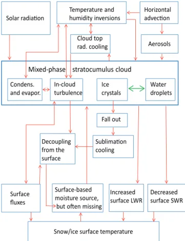
Clouds are ubiquitous in the Arctic. As mentioned in Sect. 2.1, clouds interact with the temperature and humidity inversions and affect the ABL stratification (Figs. 1 and 4), and fog (sea smoke) is often formed over leads and polynyas (Fig. 3). The cloud fraction has an annual cycle with a max-imum in early autumn and minmax-imum during late winter (e.g. Curry et al., 1996; Shupe et al., 2011). This has been ob-served since the beginning of the satellite era (Liu et al., 2012), yet atmospheric models continue to struggle with even this first-order cloud property. An ensemble average of state-of-the-art CMIP3 climate models generally agree with satel-lite observations of the Arctic cloud fraction annual cycle. In-dividually, however, models display a substantial inter-model spread, largest during winter and smallest in summer, which dramatically biases their ability to capture the correct annual cycle amplitude and some models even have an inverse an-nual cycle with less clouds in summer and more in winter (Karlsson and Svensson, 2011). Summer clouds also posed problems for the Community Atmospheric Model version 4 (CAM4) (Kay et al., 2011), and simulation of clouds was one of the main problems in testing of the Polar WRF model against SHEBA data (Bromwich et al., 2009) and recently against the Arctic Summer Cloud–Ocean Study (ASCOS) data (Wesslen et al., 2014) as part of the Arctic System
Re-Water droplets Mixed-phase stratocumulus cloud
Temperature and humidity inversions
Ice crystals
Decoupling from the surface
Cloud top rad. cooling
Increased surface LWR In-cloud
turbulence Solar radiation
Surface fluxes Condens. and evapor.
Decreased surface SWR Fall out
Sublimation cooling
Surface-based moisture source,
but often missing
Snow/ice surface temperature
Horizontal advection
Aerosols
Figure 4. Schematic diagram on the effects and interactions related to mixed-phase stratocumulus clouds and radiative transfer. Macro-and microphysical processes Macro-and interactions are shown as arrows, the green arrow representing numerous microphysical processes re-lated to aerosols, nucleation, evaporation, depositional ice growth, cloud layer glaciation, and effects of saturation vapour pressure dif-ferences of liquid and ice (see e.g. Morrison et al., 2012).
analysis effort. Models also have difficulties in representing the correct amount and vertical distribution of cloud hydrom-eteor phase partitioning over polar regions, under a wide range of annual temperatures. These biases lead to direct consequences for the surface radiation budget, near-surface temperature, and the lower ABL thermal stability and tur-bulent structure (Tjernström et al., 2008; Birch et al., 2009; Karlsson and Svensson, 2011; Kay et al., 2011; Cesana et al., 2012; Liu et al., 2012).
more frequent. The MPS clouds have a profound impact on the surface energy balance, since liquid water generates significantly more long-wave radiation to the surface than do ice clouds (Tjernström et al., 2008; Sedlar et al., 2011; Wesslen et al., 2014), and hence on the surface melt and freeze (Fig. 4). Therefore, MPS clouds will be a focus here.
An obvious connection between cloud phase and atmo-spheric temperature is present. MPS clouds are often the preferential cloud class when temperatures range between −15 to near 0◦C (Shupe, 2011; de Boer et al., 2009), but liquid water has been observed in clouds at temperatures as low as below−34◦C (Intrieri et al., 2002). Complicating the matter, the presence of liquid droplets and ice crystals to-gether forms an unstable equilibrium due to the saturation vapour pressure differences of ice and liquid, the Wegener– Bergeron–Findeisen (WBF) process (c.f. Morrison et al., 2012). Despite this instability, liquid-topped clouds with ice and/or drizzle precipitating from this layer are the norm within the lower Arctic troposphere from spring through au-tumn (Tjernström et al., 2004; de Boer et al., 2009; Shupe, 2011; Sedlar et al., 2011). Shupe et al. (2011) observed mean duration times of the order of 10 h for these cloud systems, but they may also occur as quasi-stationary systems persist-ing for days (Shupe et al., 2008; Sedlar et al., 2011; Shupe, 2011).
The generally long lifetime of MPS clouds suggests that relative humidity with respect to liquid (RHliq) is kept high within and near the cloud layer. If RHliq becomes sub-saturated in the presence of ice crystals, liquid droplets must evaporate following the WBF process, and hence would cause a rapid depositional ice growth and cloud layer glacia-tion. Instead, Shupe (2011) has shown that in-cloud RHliq and temperature distributions at a number of Arctic stations are in fact surprisingly similar, lending support for a sys-tem that is both conditioned for, and dependent upon, mixed-phase clouds. In general, stratiform clouds do not need large-scale updrafts, e.g. convection, to sustain them. Instead, these clouds rely on cloud-driven (in-cloud production of) vertical motion where the small-scale dynamics (turbulence) depends on the presence of liquid, through the cloud-top cooling, but also supplies the moisture that sustain that liquid layer.
Cloud top radiative cooling is typically very efficient as near-adiabatic liquid water content (LWC) profiles are com-mon in the Arctic (Curry, 1986; Shupe et al., 2008). Arctic MPS droplet radii generally also increase with height (e.g. Curry, 1986) and droplet effective radii often range between 4 to 15 µm. Typical LWC in MPS peaks between 0.1 and 0.2 g m−3 (McFarquhar et al., 2007) and together with rel-atively thin liquid layers (Shupe et al., 2008; Shupe 2011), cloud liquid water path (LWP) is often below 100 g m−2(de Boer et al., 2009; Sedlar et al., 2011; Shupe et al., 2011). In-cloud ice water contents (IWC) are generally largest be-tween cloud mid-level and base, decreasing upwards towards cloud top where they are initially formed (Shupe et al., 2008). Recent campaigns report a wide spectrum of ice crystal
ef-fective diameters, ranging from 20–60 µm (McFarquhar et al., 2007; Shupe et al., 2008) and upwards of 100 µm when falling through the sub-cloud layer (de Boer et al., 2009).
The ratio of LWC to total water content is often larger than 0.8 (McFarquhar et al., 2007; Shupe et al., 2008) in-dicating the resilience of cloud liquid despite near-constant drizzle and ice precipitation. In fact, de Boer et al. (2011) found evidence that liquid saturation occurs prior to ice crys-tal development even in a supersaturated environment with respect to ice. The authors suggest that ice nucleation mech-anisms in the Arctic MPS thus tend to be controlled by pro-cesses that rely on the presence of liquid condensate, further emphasising the importance of cloud motions in controlling the resilience of MPS.
In contrast to subtropical stratocumulus where decoupling between the surface and the cloud layer occurs during day-time as a part of a diurnal cycle, the Arctic ABL and sub-cloud thermodynamic structure often feature a persistent de-coupling between the surface and the cloud layers (Shupe et al., 2013), and the mechanisms are different. This de-coupling appears to be most common during the cold, dark months but also occurs during the transition and summer sea-sons (Kahl, 1990; Tjernström et al., 2004, 2012; Sedlar et al., 2011, 2012; Solomon et al., 2011; Shupe et al., 2013). Thus, the surface-based moisture source for Arctic MPS is often missing (Fig. 4). Sedlar and Tjernström (2009) and Sedlar et al. (2012) identified a common, persistent Arctic MPS cloud regime over the Arctic where the cloud layer is de-coupled from the surface, a liquid cloud top extending above the stably stratified temperature inversion base, and ice crys-tals precipitating from the cloud. They hypothesize that the presence of specific humidity inversions, a common Arctic phenomenon (see Sect. 2.1.1), are vital to Arctic MPS sur-vival. Surface turbulent heat and moisture fluxes are gener-ally small over sea ice (Persson et al., 2002; Tjernström et al., 2005, 2012), and ice crystals falling from the cloud into the sub-saturated sub-cloud layer will further enhance de-coupling due to cooling from ice crystal sublimation (Fig. 4; Harrington et al., 1999). Thus, instead of moisture originat-ing from the surface, the increased humidity within the inver-sion structure may be the moisture source which sustains the cloud system (Solomon et al., 2011; Sedlar et al., 2012).
were observed, ice production generally ceased and fewer ice crystals grew to large sizes and fell from the still-present, yet slightly more tenuous, liquid layer. Hence the coexistence of liquid and ice is intimately linked to cloud-scale motions, which in turn depends on the presence of liquid water.
Tjernström (2007) suggested that most of the boundary layer turbulence in the Arctic is in fact generated by bound-ary layer clouds, at least in summer. If the in-cloud turbu-lence production is strong and stratification below the cloud layer is weak, the cloud-induced turbulent eddies may pene-trate to the surface, hence affecting the surface fluxes of mo-mentum, heat, and moisture (Fig. 4). Cloud-generated mix-ing is found beneath cloud base, but the extent to which these turbulent motions reach the surface is often limited by a sub-cloud stable layer (Shupe et al., 2013; Sedlar and Shupe, 2014) and is also dependent on the distance from the cloud base to the surface and the sublimation of precipitation in the layer below the cloud base (Fig. 4). Hence the strongest but also most variable turbulence generation is due to buoyant cloud overturning due to cloud top cooling, which generates eddies that often persist below the cloud base. Mechanical generation of turbulence at the surface, on the other hand, is seldom very strong and intense buoyant mixing is essentially absent over sea ice (other than over winter leads/polynyas), and the ABL is therefore most often shallow. Coupling, or the lack thereof, of MPS clouds to the surface and surface fluxes are therefore more often dependent on if the cloud-generated turbulence can reach down to the ABL or not, rather than the other way around. This in turn is sensitive to the cloud-generated turbulence but also to the cloud base height (Fig. 4; Tjernström et al., 2012; Shupe et al., 2013; Sotiropoulou et al., 2014).
Spectral analysis of in-cloud vertical velocities reveals only modest changes to the cloud-generated temporal fre-quencies and horizontal wavelengths of vertical velocity when the cloud layer transitions between a surface–cloud coupled and decoupled state (Sedlar and Shupe, 2014); the authors concluded that the surface–cloud coupling state is therefore a result of the cloud processes and not dependent on the turbulence generated near the surface. Analysis of winter soundings from SHEBA in Tjernström and Graversen (2009) additionally shows how the boundary layer structure changes are almost binary between a well-mixed state, simi-lar to summer conditions when clouds containing liquid wa-ter are present, and a distinct surface inversion structure when clouds are either absent or optically thin.
In terms of temperature, the radiative cooling from the liq-uid cloud top (Harrington et al., 1999) dominates over other local processes and hence, in the absence of frontal passages or other large-scale controls, cloud droplets will continuously form to replace the water that precipitates out. Cloud droplets can persist as long as a moisture source is present. The pres-ence of humidity inversions near cloud top provide such a source (Fig. 4), and Solomon et al. (2011) describe how cloud-generated vertical motions, and small but appreciable
droplet condensation above the temperature inversion base, create the link between the cloud layer and the stable upper entrainment zone. This is a feature unique to the low-level Arctic thermodynamic structure, not observed in lower lat-itudes where large-scale subsidence generally prohibits hu-midity increases near cloud top. Furthermore, this situation is maintained by ice crystal formation and fallout (Shupe et al., 2008), effectively limiting the LWC near cloud top.
In addition to moisture, clouds need aerosol particles on which to condense and freeze (Fig. 4). These cloud con-densation nuclei (CCN) and ice nuclei largely determine the clouds’ microphysical structure and hence their radia-tive properties. Over the Arctic, where local sources of pollu-tion generally do not exist, transport in the region is consid-ered a large contributor to the concentration and composition of CCN and ice nuclei (e.g. Shaw, 1975). In winter, when the ocean is ice covered, there is a substantial transport of aerosols and aerosol precursor gases into the Arctic (Barrie, 1986; Garrett and Zhao, 2006; Lubin and Vogelmann, 2006). In summer, the meridional transport is smaller and the for-mation of low clouds and fog at the MIZ, as sub-Arctic ma-rine air adjusts to the frozen or melting surface, forms an effective filter for the transport of aerosols in the lower tropo-sphere. Thus, in the summer boundary layer the aerosol con-centrations are generally very low compared to further south (Tjernström et al., 2014) while transport of aerosols from lower latitudes may occur at higher elevations (Lance et al., 2011). While the ocean surface is more exposed in summer, local production of aerosols may be important (Tjernström et al., 2014). Low aerosol concentrations and low temperatures both contribute to a preference for optically thin clouds and also promote precipitation formation.
2.2.2 Cloud–radiation interaction
The central Arctic imposes unique boundary conditions on both shortwave (solar) and long-wave (infrared) radiative transfer, controlled by the large seasonal variations in the incoming fluxes and a wide range of surface albedo condi-tions (Sect. 3.1.2). The presence of cloud cover impacts ra-diation reaching the surface in two competing ways. First, cloud hydrometeors absorb long-wave radiation, increasing the emissivity relative to a clear-sky atmosphere. This re-sults in a net warming effect at the surface, especially over the Arctic where clear-sky effective emissivity is generally low, but simultaneously leads to cooling of the upper portion of the clouds. Conversely, clouds reflect incoming shortwave radiation to space resulting in a net surface cooling effect. Over the Arctic, the efficiency of shortwave cloud cooling is further limited by relatively large solar zenith angles (SZAs) and surface albedos; the latter is often as high as that of the overlying cloud. In fact, it still remains uncertain whether the net radiative effect of clouds in summer is to cool the surface over the large-scale Arctic Basin, even though observations from SHEBA suggest a net cloud cooling effect during June and July (Intrieri et al., 2002; Shupe and Intrieri, 2004). In an Arctic-wide sense, this net cloud effect is significantly connected to time of year, geographic location and surface albedo, notwithstanding the cloud physical properties.
The surface energy residuals, available for melting or freezing of the ice, are therefore strongly modified by the cloud radiative forcing. During ASCOS, surface energy bud-get analysis during the end of the 2008 melt season, towards the initiation of freeze-up, demonstrated the delicate inter-play of clouds, radiation, turbulence, and heat conduction in snow and ice (Sedlar et al., 2011). A week-long delay of the autumn freeze-up was realized through the manifesta-tion of a positive long-wave cloud radiative forcing of about 70 W m−2, while the shortwave radiative cooling was limited to about−40 W m−2by surface albedo and SZA constraints. Net surface energy residuals, however, were significantly re-duced by redistribution of heat and moisture via near-surface turbulence and heat conduction in snow/ice. The increase of the surface albedo, that eventually put the energy balance be-yond recovery, was not gradual but a result of heavy frost formation and melt pond freezing during a short colder pe-riod with new snowfall (Sedlar et al., 2011; Sirevaag et al., 2011; Tjernström et al., 2012). The onset of freeze-up was not realized until the low-level Arctic MPS became tenuous and cloud LWP decreased below 20 g m−2 – essentially di-minishing the cloud greenhouse effect.
Comparing various climate models, the monthly averaged spread in LWP and ice water path (IWP) in the Arctic can be as large as a factor of 3 (Karlsson and Svensson, 2011). Such variability inherently results in differences in cloud fraction as well as in the cloud–radiation interaction (Karlsson and Svensson, 2011). Tjernström et al. (2008) identified signifi-cant biases in several regional climate model simulations of
surface radiative fluxes during SHEBA. Both downwelling shortwave and long-wave radiation were negatively biased, while the bias magnitudes varied depending on the model. Tjernström et al. (2008) found a significant underestima-tion (overestimaunderestima-tion) in cloud LWP above (below) 20 g m−2. Conversely, nearly all models underestimated the IWP and there were clear biases in the model simulations of liquid to total cloud water path. The authors speculated that the biases in downwelling long-wave radiation might be due to an absence of sufficient liquid water in winter and that the downwelling shortwave radiation bias was due to too-opaque clouds, i.e. too-high cloud albedo. However, even when the actual errors in LWP and IWP were cancelled in the analysis a bias remained. Thus, even if the distribution of ice and liquid were properly resolved, the modelled cloud-radiation interaction tends to be misrepresented, and this er-ror will propagate to surface radiation balance erer-rors for the ice and the ocean in coupled Earth System Models. These results point at the importance of a proper handling of the aerosol/cloud/radiation feedback in resolving the proper ra-diation balance at the surface (Sect. 5.3).
2.3 Partly resolved processes 2.3.1 Coastal and fjordic features
Coastal regions and in particular coastal mountain ranges can have a pronounced impact on the mesoscale and boundary layer meteorology of the adjacent coastal waters. This impact arises from the combined effects of orography and spatial differences between the surface temperatures of snow/ice-covered land, sea ice, and the open ocean. Considering oro-graphic effects, when the wind is flowing towards a bar-rier it must either rise over it or be distorted by it, i.e. it turns to flow along the coast as a barrier wind or related feature, such as a tip jet (common near the southern tip of Greenland). On the downstream side of a barrier there is of-ten some sort of orographic forcing mechanism leading to mesoscale features such as gap winds, katabatic winds, foehn winds or wake effects. The surface temperature differences affect the thermodynamics of the ABL and further the wind field, sometimes also generating mesoscale circulations. All of these mesoscale phenomena are only partially resolved in current climate models and global NWP models, although NWP models can adequately simulate these features if ap-propriate parameterizations are used and the grid size is suf-ficiently small.
winds off southeastern Greenland are documented in Pe-tersen et al. (2009). They found barrier-effect enhancements of up to 20 m s−1and peak wind speeds of up to 40 m s−1. The structure of the barrier winds was strongly dependent on the synoptic-scale situation, often consisting of a cold bar-rier jet undercutting a warmer maritime air mass and gener-ally with a significant ageostrophic component of the flow. A climatology of these barrier winds shows that they occur typically once a week, but with a large interannual variability determined primarily by the broader-scale situation (Harden et al., 2011). Off SE Greenland, there are two distinct areas of occurrence (Harden et al., 2011). Idealized numerical sim-ulations (Harden and Renfrew, 2012) and reanalyses work (Moore, 2012) have shown that these two areas are related to two areas of steep topography, separated by a major fjord. In SE Greenland, barrier winds are known to play a key role in generating a fjordic ocean circulation leading to submarine melting and thus the rapid retreat of ice shelves that is now being seen there (Straneo et al., 2010).
The first in situ observations of a tip jet off Cape Farewell, Greenland documented near-surface winds of over 35 m s−1 and peak jet winds of almost 50 m s−1 (Renfrew et al., 2009a), while a dynamical analysis of these events showed their characteristic curve around the “tip” was associated with a collapse in the cross-jet pressure gradient as the bar-rier decreases in height (Outten et al., 2009, 2010). Tip jets are also found off Svalbard (e.g. Reeve and Kolstad, 2011), and over the Bering Sea (Moore and Pickart, 2012); while gap flows were observed by an instrumented aircraft in the Svalbard region during the Norwegian IPY-Thorpex experi-ment (Barstad and Adakudlu, 2011).
There are generally very high winds associated with all of these coastal jet features, so consequently there are ele-vated momentum fluxes and often eleele-vated heat and moisture fluxes, depending on the source of the air, i.e. the air–sea tem-perature difference. Petersen and Renfrew (2009) provided observations from six GFDex flights into tip jets and barrier winds using the eddy covariance method and found fluxes up to 1.9 N m−2(momentum), 300 W m−2 (sensible heat), and 300 W m−2(latent heat). These are among the highest fluxes ever directly measured and certainly significant enough to lead to enhanced ocean mixing, water mass changes, and po-tentially circulation changes in the ocean (e.g. Våge et al., 2008; Haine et al., 2009, Sproson et al., 2010). Although large air–sea heat fluxes are not always the case; the heat fluxes associated with Greenland’s easterly tip jets tend to be more moderate and are not associated with the deep open ocean convection events that tend to occur in the SE Labrador Sea (Sproson et al., 2008).
The spatial variability of atmospheric variables within a fjord may be very large (Fig. 5). For Svalbard fjords, Kilpeläinen et al. (2011) reported that variability can reach levels comparable to the synoptic-scale temporal variability. The contribution of surface type to the spatial variability of turbulent heat fluxes increases with increasing air–sea
tem-Figure 5. Examples demonstrating large spatial variations in air temperature and wind (a and b) and sensible heat flux (c and d) over a complex fjord (Isfjorden in Svalbard, length approx-imately 100 km), as simulated applying a high-resolution atmo-spheric model. Redrawn with permission from Kilpeläinen (2011).
presence of sea ice cover was found as a very important fac-tor for determining whether a katabatic flow can reach the fjord surface or be elevated above the stable boundary layer (Vihma et al., 2011). Effects of sea ice cover on spatial varia-tions in the ABL over a Svalbard fjord were also detected by Láska et al. (2012).
Orographic effects are sometimes responsible for the gen-esis of polar mesoscale cyclones, e.g. in the case of lee cy-clones southeast off Greenland. In most cases, however, po-lar mesoscale cyclones are not directly related to orographic forcing and are discussed in a separate section below.
2.3.2 Mesoscale cyclones
Polar mesoscale cyclones are vortices north of the main po-lar frontal zone, with the most intense ones (near-surface wind speeds more than 15 m s−1) being classified as polar lows. They are typically short-lived (12–48 h in duration) and generally occur over the subpolar seas. They fall broadly into two classes: those that are fundamentally convective, i.e. forced by large air–sea heat fluxes, and those that are fun-damentally baroclinic, i.e. instabilities of a horizontal tem-perature gradient, often associated with Arctic fronts. In re-ality, most polar mesoscale cyclones have a mixture of these forcing mechanisms at different stages of their life cycle. Po-lar mesoscale cyclones tend to occur over the sub-poPo-lar seas, e.g. the Greenland, Norwegian, Iceland, Barents, Irminger, Labrador, and Bering seas, the Sea of Japan, and the Gulf of Alaska in the Northern Hemisphere. Further background can be found in, e.g. Renfrew (2003) and Rasmussen and Turner (2003).
In recent years there has been an upsurge of interest in po-lar lows. The IPY was a focal point for a number of field cam-paigns which observed polar lows, including GFDex (e.g. Renfrew et al., 2008) and the Norwegian IPY-Thorpex cam-paign (Kristjánsson et al., 2011). In the latter, arguably the most comprehensive set of observations of a polar low to date were obtained for a case over the northern Norwegian Sea, enabling studies of the structure, dynamics, lifecycle, simulation accuracy, and predictability of this event (e.g. Lin-ders and Saetra, 2010; Føre et al., 2011; Føre and Nordeng, 2012; McInnes et al., 2011; Wagner et al., 2011; Irvine et al., 2011; Aspelien et al., 2011; Kristiansen et al., 2011). Find-ing, for example, that this case had critical upper-level forc-ing (Føre et al., 2011), and was more accurately simulated with a convection-permitting grid resolution of 4 or 1 km (McInnes et al., 2011). Operational weather forecasting sys-tems have now reached the state where polar lows should be able to be predicted routinely. Numerical weather prediction grid sizes have been adequate for some time, but observing and data assimilation systems have not always been able to consistently provide suitable initial conditions; for example, in Irvine et al. (2011) there was strong sensitivity to the ini-tial conditions. Regional high-resolution ensemble prediction systems (EPS) provide a realistic prospect of robust
predic-Figure 6. Differences in the monthly maximum depth of open-ocean convection in open-ocean model experiments with and without po-lar lows included in the atmospheric forcing (a) the Greenland Sea and (b) the Norwegian Sea. Reproduced with permission from Con-dron and Renfrew (2013).
tions at the mesoscale, tackling initial condition sensitivity for example. These regional EPS systems are still being de-veloped and optimizing their setup for polar lows is a current challenge (Aspelien et al., 2011; Kristiansen et al., 2011). For example, Kristiansen et al. (2011) found a crucial depen-dence on EPS domain size and location, as well as on certain parameterization settings.
Polar mesoscale cyclones are not explicitly resolved by the current generation of global climate models. Due to their high impact, predictions of any changes in frequency or loca-tion of occurrence are important. A couple of recent studies address this: Kolstad and Bracegirdle (2008) use marine cold air outbreaks as a proxy for polar low activity; while Zahn and von Storch (2010) use dynamical downscaling to sim-ulate polar mesoscale cyclones. In both studies a migration northwards is found, following the retreating sea ice pack, and consequently there is a decrease in the frequency of po-lar lows through the 21st century.
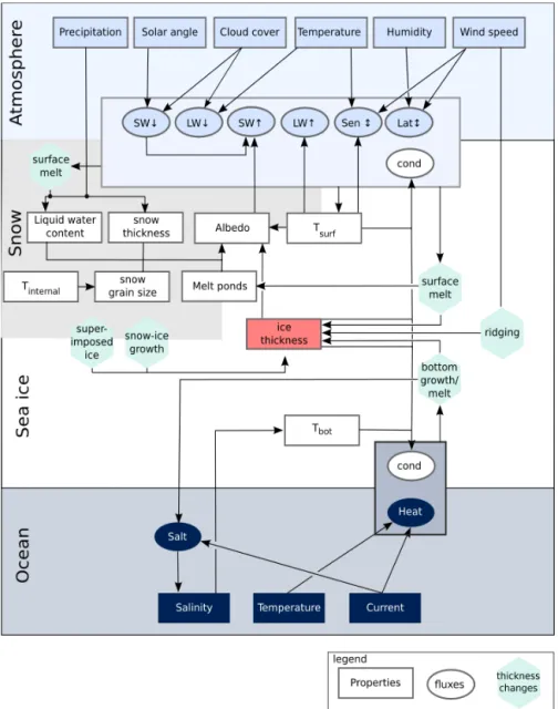
Figure 7. Schematic overview of some of the processes that influence and are influenced by the growth and melt of sea ice. Only the most important pathways of interaction are shown. SW is shortwave radiation, LW is long-wave radiation, Lat is latent heat flux, Sen is sensible heat flux, Cond is conductive heat flux in the ice, Heat is oceanic heat flux, Salt is oceanic salt flux,Tbotis ice bottom temperature, andTsurf is surface temperature.
up the Greenland Sea gyre, and increases the momentum and heat transported north in the North Atlantic subpolar gyre as well as the frequency of dense water flowing south out of the Nordic seas. The impact of polar lows on the coupled cli-mate system is still uncertain: their occurrence is subject to changes in both the atmosphere and ocean, and any changes will potentially feedback on both the atmosphere and ocean.
3 Sea ice and snow
3.1 Radiative processes and properties 3.1.1 Melt onset