www.ocean-sci.net/11/743/2015/ doi:10.5194/os-11-743-2015
© Author(s) 2015. CC Attribution 3.0 License.
Transport of volume, heat, and salt towards the Arctic in the Faroe
Current 1993–2013
B. Hansen1, K. M. H. Larsen1, H. Hátún1, R. Kristiansen1, E. Mortensen1, and S. Østerhus2 1Faroe Marine Research Institute, Tórshavn, Faroe Islands
2Uni Research Climate, Bergen, Norway
Correspondence to:B. Hansen ([email protected])
Received: 24 April 2015 – Published in Ocean Sci. Discuss.: 9 June 2015
Revised: 29 August 2015 – Accepted: 8 September 2015 – Published: 22 September 2015
Abstract. The flow of warm and saline water from the At-lantic Ocean, across the Greenland–Scotland Ridge, into the Nordic Seas – the Atlantic inflow – is split into three sepa-rate branches. The most intense of these branches is the in-flow between Iceland and the Faroe Islands (Faroes), which is focused into the Faroe Current, north of the Faroes. The Atlantic inflow is an integral part of the North Atlantic ther-mohaline circulation (THC), which is projected to weaken during the 21st century and might conceivably reduce the oceanic heat and salt transports towards the Arctic. Since the mid-1990s, hydrographic properties and current velocities of the Faroe Current have been monitored along a section ex-tending north from the Faroe shelf. From these in situ obser-vations, time series of volume, heat, and salt transport have previously been reported, but the high variability of the trans-port has made it difficult to establish whether there are trends. Here, we present results from a new analysis of the Faroe Current where the in situ observations have been combined with satellite altimetry. For the period 1993 to 2013, we find the average volume transport of Atlantic water in the Faroe Current to be 3.8±0.5 Sv (1 Sv=106m3s−1)with a heat transport relative to 0◦C of 124±15 TW (1 TW=1012W). Consistent with other results for the Northeast Atlantic com-ponent of the THC, we find no indication of weakening. The transports of the Faroe Current, on the contrary, increased. The overall increase over the 2 decades of observation was 9±8 % for volume transport and 18±9 % for heat transport (95 % confidence intervals). During the same period, the salt transport relative to the salinity of the deep Faroe Bank Chan-nel overflow (34.93) more than doubled, potentially strength-ening the feedback on thermohaline intensity. The increased heat and salt transports are partly caused by the increased
volume transport and partly by increased temperatures and salinities of the Atlantic inflow, which have been claimed mainly to be caused by the weakened subpolar gyre.
1 Introduction
The flow of warm and saline water from the Atlantic Ocean, across the Greenland–Scotland Ridge, into the Nordic Seas, theAtlantic inflow, occurs in three separate branches (plus
flow over continental shelf areas). The two main branches pass between Iceland and the Scottish shelf on either side of the Faroes (Faroe Islands). This study treats the branch that flows between Iceland and the Faroes, theIF inflow(Fig. 1a),
across the Iceland-Faroe Ridge (IFR) and continues in the
Faroe Current.
This flow carries heat towards the Arctic and is an in-tegral part of the North Atlantic thermohaline circulation (THC), which is projected to weaken due to global warming (Collins et al., 2013). It has therefore long been an ambition to monitor its transport of water (volume, mass), heat, and salt. The hydrographic properties (temperature and salinity) of the Faroe Current have been monitored along a section,
section N, extending northwards from the Faroes since the
late 1980s. In the mid-1990s, this section was instrumented with moored Acoustic Doppler Current Profilers (ADCPs) to monitor the transports (Fig. 1b). During and after crossing the IFR, the Atlantic water meets and mixes with colder and less saline water masses, which here are collectively termed
Arctic water. In this study, we focus on the Atlantic water
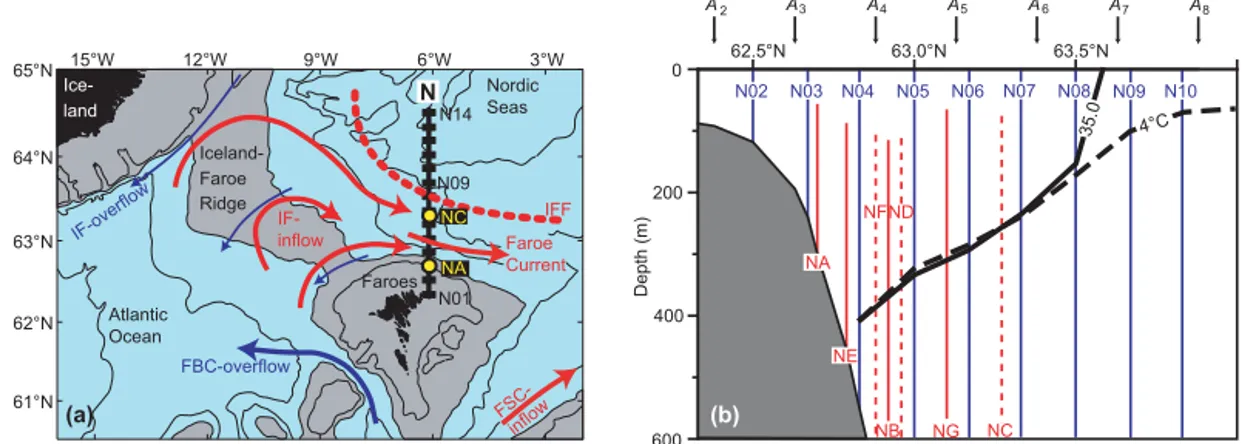
Figure 1. (a)The region between Iceland and the Scottish shelf with gray areas shallower than 500 m. The two main Atlantic inflow branches are indicated by red arrows. The Iceland–Faroe inflow (IF inflow) crosses the IFR, meets colder waters, termed Arctic water, in the Iceland-Faroe Front (IFF), and flows north of Iceland-Faroes in the Iceland-Faroe Current. The other main inflow branch (the FSC inflow) is also shown. The black line extending northwards from the Faroe shelf is section N with CTD standard stations N01 to N14 indicated by black rectangles. Yellow circles indicate the innermost (NA) and the outermost (NC) ADCP mooring sites on the section. Blue arrows indicate deep overflow into the Atlantic.(b)The southernmost part of section N with bottom topography (gray). Standard CTD stations are indicated by blue lines labeled N02 to N10. ADCP profiles are marked by red lines that indicate the typical range with continuous lines indicating the long-term sites. Altimetry grid points A2to A8are marked by black arrows and the thick black lines indicate the average depth of the 4◦C isotherm (dashed) and the 35.0 isohaline (continuous) on the section.
A priori, it might seem inappropriate to locate the moni-toring section downstream of the IFR rather than on it. The ridge is, however, wide and inflow has been reported to oc-cur over most of its width (Orvik and Niiler, 2002; Jakobsen et al., 2003; Rossby et al., 2009). Strong mesoscale activ-ity and the counterflow of cold overflow water (IF overflow) below the Atlantic water also requires high spatial resolu-tion of velocity as well as temperature and salinity measure-ments. Monitoring on the IFR would therefore require a pro-hibitively large number of moorings, which would have to be protected from fishing gear. The chosen monitoring sec-tion, section N, in contrast, has a much more focused inflow, where most of the ADCPs may be deployed sufficiently deep to avoid loss from fishing gear. Only over the relatively nar-row Faroe slope is it necessary to protect the ADCPs by bot-tom mounted frames (sites NA and NE on Fig. 1b).
After some initial experimentation, monitoring started in summer 1997 with an ADCP array with three moorings (NA, NB, and NC). The array has been altered and mooring sites have been changed, but as a whole, it has continued oper-ating since then, although with gaps during annual servic-ing and due to instrument failure or loss. In parallel, regular CTD (conductivity, temperature, depth) cruises have gath-ered hydrographic data at standard stations (Fig. 1), usually 3–5 times a year.
Based on the combined CTD and ADCP data sets, time series of volume transport and heat and salt transport were reported in Hansen et al. (2003) for the 1997–2000 period and in Hansen et al. (2010) for the 1997–2008 period. In both cases, the transport values were based on the in situ data (CTD and ADCP), solely, using the methodology described
in Hansen et al. (2003). It appeared that there was good corre-spondence between these in situ based estimates and satellite altimetry (Hátún and McClimans, 2003; Hansen et al., 2010) and it was recognized that better estimates might be made by combining the in situ observations with satellite altimetry.
We have therefore re-analyzed the complete updated data set including both the in situ data and altimetry data from a line of grid points parallel to and close to the monitoring section (Fig. 1b). This task involves a large number of tech-nical issues that will not be detailed here. These details are described in a Supplementary document, which we will refer to repeatedly. In this paper, we focus on the main results from the analysis, which are the time series of volume, heat, and salt transport by the Atlantic water component of the Faroe Current. We report average values and estimate seasonal vari-ations, but the main aim is to resolve, whether any of the transport series exhibit overall trends over the observational period, and to quantify them.
2 Material and methods
All the in situ observations (available at www.envofar.fo) were collected along section N (Fig. 1). Altimetry data are selected along a line following longitude 6.125◦W, which is so close that we consider it to be along the same section. 2.1 Hydrographic observations
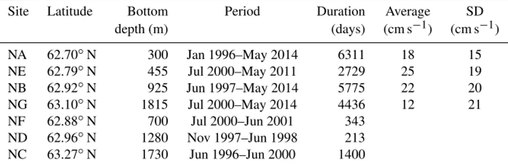
Table 1.Main characteristics of the measurements at the seven ADCP sites. For the four long-term deployment sites, the table also lists
averages and standard deviations of the extrapolated eastward surface velocity.
Site Latitude Bottom Period Duration Average SD depth (m) (days) (cm s−1) (cm s−1)
NA 62.70◦N 300 Jan 1996–May 2014 6311 18 15 NE 62.79◦N 455 Jul 2000–May 2011 2729 25 19 NB 62.92◦N 925 Jun 1997–May 2014 5775 22 20 NG 63.10◦N 1815 Jul 2000–May 2014 4436 12 21 NF 62.88◦N 700 Jul 2000–Jun 2001 343
ND 62.96◦N 1280 Nov 1997–Jun 1998 213 NC 63.27◦N 1730 Jun 1996–Jun 2000 1400
64.5◦N (N14 is at longitude 6.000◦W). Properties at these stations are labeled by the indexj (j=1 to 14). Typically, the section has been occupied on four cruises each year since 1988 although bad weather and other conditions have pre-vented complete coverage in some cases. Thus, some stations have been occupied almost a hundred times, but others con-siderably less often, especially in the northernmost part.
We use quality-controlled and calibrated CTD data aver-aged to meter intervals with a main focus on data between stations N02 and N11, which contain that part of the section through which the Atlantic water passes. Accuracy is better than 0.01◦C for temperature and 0.01 for salinity through-out the period although salinity spikes in strong thermoclines may exceed this threshold prior to 1997 when the high qual-ity (SeaBird 911+) CTD model was first acquired.
2.2 In situ current velocity observations
Between January 1996 and May 2014, ADCPs have been moored at seven different sites along the section (Table 1). Each site is labeled by a two-letter code beginning with “N”. At two sites (NF and ND), only single deployments were made. The other sites have had repeated deployments, with moorings usually deployed in summer one year and re-covered the year after. Thus, there are typically gaps of 2– 4 weeks every summer.
The most complete coverage has been when all four “long-term” sites (NA+NE+NB+NG) were occupied, from summer 2000 to summer 2001 and from summer 2004 to summer 2011. At most sites, the ADCPs have been deployed in the top of traditional moorings at sufficient depth to pre-vent loss from fishing gear. At the shallow sites, NA and NE, it has been necessary to put the ADCPs into protective buoy-ant frames attached by acoustic releases to concrete anchors deployed on the bottom (Fig. S2.2.1 in the Supplement). The ADCPs have typically pinged every 20 min (single pings).
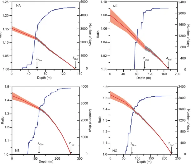
After extensive editing and quality control, the data have been averaged to daily values with accuracy ≈0.2 cm s−1. From the observations, we find that the shape of the ADCP profiles at each site is very consistent so that the ratio be-tween eastward velocities at two different depths is relatively
constant in time (Fig. 2). Using observed and extrapolated values for this ratio (Fig. 2), we have extrapolated all the profiles from the long-term sites to the surface. We also use the bottom temperature measured by the ADCP temperature sensor at site NE,TNE, close to the typical boundary between Atlantic and Arctic water masses (Fig. 1b). This sensor may have offsets several tenths of a degree, but that is adequate for our purpose.
2.3 Satellite altimetry
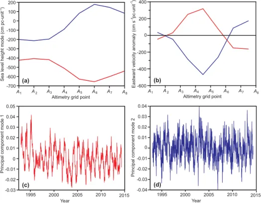
Daily averaged altimetry was selected from the global grid-ded (0.25◦×0.25◦) AVISO+ sea level anomaly (SLA) field produced by Ssalto/Duacs and distributed by Aviso with support from Cnes (http://www.aviso.altimetry.fr). We have used the DT MSLA “all sat merged” data set (http://www.aviso.altimetry.fr/fileadmin/documents/data/ tools/hdbk_duacs.pdf). SLA values were selected for 8 grid points, which we label A1 to A8, along 6.125◦W from 62.125 to 63.875◦N (Fig. 1b). We use the index k (k=1 to 8) to identify these points. For each of these points, we have sea level anomaliesHk(t ) for 7791 days from 1 Jan-uary 1993 to 1 May 2014. An empirical orthogonal function (EOF) analysis on the SLA values from these eight points re-vealed that the first two modes explained 95 % of the variance with 87 % in the first mode (Fig. 3). The associated princi-pal components (temporal variation) are denoted PC1(t )and PC2(t ), respectively. The EOF modes also revealed that the flow variations are confined to the region north of A2, which is the region we will focus on.
At timescales exceeding a few days, we expect approx-imate geostrophic balance, so that the horizontally aver-aged eastward surface (z=0) velocityUk(0, t )between grid points Akand Ak+1 is proportional to the difference in
Figure 2.Vertical variation of eastward velocity for the long-term ADCP sites. Each panel shows for one of the long-term ADCP sites, the number of days with data at each depth (blue curve, right scale) and the ratioU (z, t )/U (zRef, t )(red curve, left scale). Here,U (z, t )is eastward velocity at depthzfor timetandzRefis the depth, up to which all profiles from the site are complete. Profiles with|U (zRef, t )|< 10 cm s−1are excluded. Fromz
Refup to the depthzObs, the ratio represented by the red curve is the average ratio based on observed ADCP profiles and the shaded gray area is±one standard error. AbovezObs, graphical extrapolation is applied up to 50 m depth. From there to the surface, the red curve is based on average geostrophic profiles. The shaded red area is graphically extrapolated from the gray area and indicates uncertainty.
each interval: Uk(0, t )=
g
f·L·
Hk(t )−Hk+1(t )
+Uk0, (1)
whereg andf are gravity and Coriolis parameter, respec-tively, andLis the distance between the altimetry grid points. The constantsUk0for each altimetry interval could be deter-mined from the mean dynamic topography (MDT), available from AVISO, but this would have given a surface current that was broader and considerably weaker than indicated by our in situ observations, especially between A3 and A5, where most of the Atlantic water transport occurs (Fig. S2.4.4). In-stead, we use values forUk0that are determined from ADCP data and average geostrophic profiles that are derived from the CTD data as elaborated in Sect. 3.1.
2.4 Combining ADCP and altimetry to generate velocity at depth
Once calibrated by Eq. (1), the altimetry data provide us with a time series of horizontally averaged eastward surface veloc-ityUk(0,t )for each altimetry interval Akto Ak+1. To find the
horizontally averaged velocityUk(z, t )for intervalkat depth z, we multiply the surface velocity Uk(0, t ) by a function ϕk(z, t ), which we term therelative profile:
Uk(z, t )=Uk(0, t )·φk(z, t ). (2) If, in a certain period, there is one ADCP that is considered to represent the altimetry intervalk, then we may assume that:
as long as uADCP (0, t ) is not too close to zero. Much of the time, we have to replaceϕk(z, t )by an average relative profile 8k(z) for each interval, however. The average rel-ative profiles are based on average ADCP profiles and on average geostrophic profiles, calculated from the CTD data (Fig. S3.2.2).
2.5 Calculation of transport time series
With the eastward surface velocityUk(0,t )determined from calibrated altimetry by Eq. (1) and its vertical variation Uk(z, t )given by Eq. (2), time series of volume transport, Q(t ), between grid points A2and A8, may be determined as:
Q(t )= 7 X
k=2 600 X
z=1
Uk(z, t )·Wk(z, t ), (4) whereWk(z, t )is the width of the interval from Akto Ak+1at
depthzand timet. If we want to integrate down to 600 m all along the section, then Wk(z, t )=L,the distance between grid points, for all k,z, andt, except where the bottom is shallower than 600 m. More generally, we may wish to in-tegrate down to a certain boundary (e.g., the 4◦C isotherm) that varies in depth along the section and also with time. In that case, we can writeWk(z, t )=L·rk(z, t )whererk(z, t ) is the fraction (between 0 and 1) of the width of altimetry intervalkat depthzthat is above the boundary or bottom at timet.
To calculate heat transport relative to a specified reference temperatureTRef, we use:
QHeat(t ) (5)
=ρ·CH· 7 X
k=2 600 X
z=1
[Tk(z, t )−TRef]·Uk(z, t )·Wk(z, t ),
whereρis density,CHis the specific heat, andTk(z, t )is the temperature at depthzand timet, horizontally averaged from Akto Ak+1.
The salt transport through section N by Atlantic water is well defined in an absolute sense. Every cubic meter passing across the IFR with a practical salinitySrepresents an input of salt to the Nordic Seas (Fig. 1a) equal toρ·CS·Skg where CSis a (approximately constant) factor converting from prac-tical to absolute salinity. The salt transport, relative to some specified reference salinitySRef, is therefore given by:
QSalt(t ) (6)
=ρ·CS· 7 X
k=2 600 X
z=1
[Sk(z, t )−SRef]·Uk(z, t )·Wk(z, t ).
3 Results
The basic results of this study are the characteristics of the velocity field, generated by combining ADCP and altimetry
data, and the characteristics of the temperature and salinity fields, mainly based on the CTD observations. By combin-ing these results, we can produce continuous time series of Atlantic water characteristics (T and S) and spatial extent on the section and we can simulate distributions of velocity, temperature, and salinity with reasonable accuracy. Together, these series allow us to generate the main results: continuous time series of volume, heat, and salt transport for the whole altimetry period.
3.1 Velocity distribution on the section
The average velocity profiles from the ADCPs and from geostrophy (Fig. 4) are compatible. We also find that the rel-ative profiles – theϕk(z, t )functions introduced in Sect. 2.4 – are consistent in shape. This is verified by correlating the ex-trapolated eastward surface velocity and the vertically aver-aged eastward velocity for individual long-term ADCP sites. For weekly averages, we find correlation coefficients be-tween 0.94 and 0.98 (Table S3.2.1 and Fig. S3.2.1 in the Supplement). This indicates that replacingϕk(z, t )by the av-erage relative profile8k(z)in Eq. (2) should generally be a good approximation.
After extrapolation to the surface, average eastward veloc-ities for the four long-term ADCP sites (Table 1) combined with more scattered observational evidence in the Faroe shelf region give a consistent picture of the horizontal variation of the average eastward surface current (black curve in Fig. 5). Farther north on the section, average geostrophic profiles combined with deep current measurements complete this pic-ture (blue lines in Fig. 5). By averaging over each altimetry interval, this leads to values forUk0fork=2 to 7 (red line in Fig. 5).
3.2 Temperature and salinity distributions
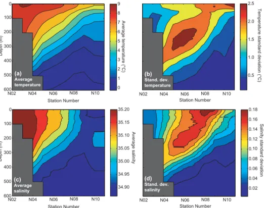
In the CTD data set, there are 78 cruises with complete cov-erage from station N02–N11 in the period 1993–2013. The average temperature (Fig. 6a) and salinity (Fig. 6c) distribu-tions on the section illustrate the characteristic difference be-tween the warm and saline Atlantic water and the colder and less saline Arctic water masses except that seasonal heating blurs the water mass characteristics in the uppermost layers in the northern part of the section (Fig. S4.1).
Seasonal heating is also indicated by a relatively high standard deviation of temperature in the near-surface layer, but the highest standard deviations for both temperature and salinity are in the pycnocline region (Fig. 6b and d) and il-lustrate variations in Atlantic water extent.
Figure 3.The first two EOF modes of the altimetry data and their principal components.(a)SLA mode 1 (red) and 2 (blue).(b)The eastward
surface velocity anomaly associated with SLA mode 1 (red) and 2 (blue) using Eq. (1) withUk0=0.(c)Principal component of SLA mode 1, PC1(t ).(d)Principal component of SLA mode 2, PC2(t ).
Figure 4. Average eastward geostrophic velocity profiles (black)
between each pair of neighboring standard stations from N03 to N07 and eastward ADCP velocity profiles from all sites (red). The surface expressions of the geostrophic profiles are located in the middle of the associated station pairs. For the long-term sites, the profiles have been extrapolated to the surface where they are located at the ADCP positions.
(frontal variations). In the next three sections, we try to esti-mate these.
3.2.1 Atlantic water temperature and salinity
As seen in Fig. 6, the southernmost stations over the shelf and inner slope are usually dominated by Atlantic water (reddish colors) and this region has also been most frequently
sam-pled in the CTD cruises. We have therefore generated time series of Atlantic water temperature and salinity by averag-ing between 100 and 150 m depth at station N03. These time series are termedTA(t )andSA(t ).
For both of these parameters, we have extracted the sea-sonal (Fig. S4.5.3) and the interannual variations (Fig. 7) us-ing an iterative procedure (Appendix B in the Supplement). The Atlantic water temperature increased about 1◦C from 1993 to 2003, after which there are no consistent trends. The salinity changes of the Atlantic water parallel the tempera-ture changes with an overall increase of about 0.1.
3.2.2 Atlantic water extent on the section
In this study, we define Atlantic water to be water that has recently crossed the IFR. In order to include only this com-ponent of the volume, heat, and salt transports, Eqs. (4)–(6) require that we are able to establish a boundary between the Atlantic and the Arctic domain on the section at any time. In reality, this boundary will be diffuse and different methods may be used to solve this (Hansen et al., 2003) but they all suffer from lack of sufficiently comprehensive hydrographic observations.
Figure 5.Values for the altimetry offsetUk0 (red line) plotted to-gether with average values for eastward surface velocity from the four long-term ADCP sites (rectangles) and from average geostro-phy (Table S2.4.3) (blue line). South of site NA, the velocity is esti-mated from various scattered observations (Fig. S2.4.4). The black curve shows a graphical interpolation from this region and between ADCP sites and values forU20,U30, andU40are averaged from these. The value forU50is a combination of ADCP site NG and geostro-phy between N06 and N07 (blue line). Values forU60andU70are based on geostrophy combined with deep current measurements (Table S2.4.3).
boundary between the Atlantic and the Arctic domain on the section. The amount of Arctic water that has been mixed into the area above this isotherm should be similar to the amount of Atlantic water that has been mixed below it. The depth of this isotherm at stationj and timet is denotedDj(t ).
From direct observations, we only know the depth of this isoline at the times of CTD cruises. As shown by Hátún et al. (2004), the temperature (and salinity) field is, however, linked to the velocity field, which again is linked to the al-timetry. To investigate this, all CTD cruises since 1993 were analyzed to find the depth of the 4◦C isotherm at stations N04–N11. No clear overall trend or seasonal variation were evident (Fig. S4.2.1). These depth values were then corre-lated with various parameters that might be considered to in-fluence isotherm depth (Table S4.2.1).
For most stations, the altimetry data provided the best in-dicator of the 4◦C isotherm depth and a multiple linear re-gression on two separate altimetry parameters could explain between 56 and 65 % of the variance in 4◦C isotherm depth for the five stations from N05 to N09. For stations N10 and N11, the explained variance decreased to 47 and 42 %, re-spectively (Table S4.2.1).
For station N04, only 30 % of the 4◦C isotherm depth variance could be explained by altimetry and ADCP veloc-ity data, solely, but the inclusion of bottom temperature ob-served at ADCP site NE increased the explained variance to 58 %. This site is located where the thermocline typi-cally intersects the bottom (Fig. 1b) and the bottom temper-ature exhibits large variations – even on monthly timescales (Fig. S4.3.1) – that indicate Atlantic water extent in the area.
Using the coefficients from these regression analyses, the depth of the 4◦C isotherm at most stations,D
j(t ), may be simulated with reasonable accuracy for every day with al-timetry data, i.e., since 1 January 1993. Especially for days in this period with bottom temperature measurement at site NE, we can simulate the 4◦C isotherm depth from its inter-sect with the Faroe slope north to station N09, explaining more than half of its total variance.
At station N09, the isotherm already approaches the sur-face and has diverged from the 35.0 isohaline (Fig. 1b). Here, temperature is no longer a good indicator of Atlantic water extent. To simulate the northern boundary of the Atlantic wa-ter extent, we instead seek to simulate the location of the 35.0 isohaline in the near-surface layer (Fig. 1b). This was also explored by multiple linear regressions on various altimetry parameters using CTD observations from the 1997 to 2013 period, for which the salinity data have the best quality.
Based on this, an algorithm was developed that allowed simulation of the latitude of the 35.0 isohaline at 100 m depth from altimetry data, explaining 44 % of its variance (Fig. S4.4.1). This is used to determine the northern bound-ary of the Atlantic water extent for the top 100 m layer.
As elaborated in Sect. 3.6, the choice of boundary for At-lantic water extent is a dominant source of uncertainty for av-erage transport estimates. Since the regression equations for Dj(t )include mainly altimetry parameters (Table S4.2.2), our results are not, however, very sensitive to changes in the Atlantic water properties. Thus, this choice should not intro-duce appreciable uncertainties to the temporal variations and trends of the transport series.
3.2.3 Simulating daily temperature and salinity fields With continuous simulation of the boundary of Atlantic wa-ter extent, Eqs. (1)–(4) allow calculation of the volume trans-port of Atlantic water, but for heat and salt transtrans-port, we need continuous simulations of temperature and salinity dis-tributions on the section, as well. To develop these, we used the CTD data from all the 78 cruises 1993–2013 that had complete coverage from station N02–N11. We found that the temperature distribution is well explained as a linear combi-nation of a seasonal signal, the Atlantic water temperature, TA(t )(Fig. 7) and the depth of the 4◦C isothermDj(t ). For stations N04 to N11, the temperatureTj(z, t ) at station j, depthz, and timetis expressed as:
Tj(z, t ) (7)
=TjSeas(z, t )+aj(z)·TA(t )+bj(z)·Dj(t )+cj(z).
Figure 6.Hydrographic conditions on section N based on 78 CTD sections in the period 1993 to 2013.(a)Average temperature;(b)standard deviation of temperature;(c)average salinity;(d)standard deviation of salinity. Gray areas indicate the bottom.
instead of Dj(t )in Eq. (7). The explanatory power of this expression varies across the section, but over the average At-lantic water extent, Eq. (7) explains 61 % of the total vari-ance, on average (Fig. S4.6.2).
For salinity, the seasonal variation is less pronounced (Fig. S4.8.1). To simulate the salinity at station j (j=4 to 11), depthz, and timet,Sj(z, t ), we therefore use the expres-sion:
Sj(z, t )=dj(z)·SA(t )+ej(z)·Dj(t )+fj(z), (8) whereSA(t )is the salinity of the Atlantic water (Fig. 7) and d,e, andf are regression coefficients. At stations N02 and N03,Dj(t )is again replaced by PC1(t ). On average over the average Atlantic water extent, Eq. (8) explains 47 % of the total variance in the observed salinity (Fig. S4.8.2).
3.3 Volume transport 3.3.1 Total volume transport
Once appropriate choices for the relative profile functions ϕk(z, t )and8k(z)have been made for each altimetry inter-valk(Table S5.3.1), Eqs. (1)–(4) allow calculation of volume transport, as long as theWk(z, t )functions are specified. As a test case, we consider the volume transport from the surface to 500 m and from N02 (midway between A2and A3)out to A8 (Fig. 1b), which we here denote total volume transport. This requiresW2(z, t )=L/2 andWk(z, t )=Lfork=3 to
7 for all depthsz=1 to 500 (or bottom where shallower). Outside of this areaWk(z, t )=0.
From 1 January 1993 to 1 May 2014, there are 223 weeks for which we have altimetry data, as well as data from all four long-term ADCP sites (NA, NE, NB, and NG). For these weeks, we can compare transport estimates based on the in-stantaneous relative profilesϕk(z, t )with estimates based on the average relative profiles 8k(z). For monthly (4-week) averages, the correlation coefficient between these two es-timates is 0.94 with an average difference of 0.03 Sv and a rms (root-mean-square) difference of 0.3 Sv (Table S5.3.2). This is 6 % of the average volume transport and well below its estimated uncertainty (Sect. 3.6).
This implies that the average relative profiles8k(z)may be used instead ofϕk(z, t ) without appreciable error. More importantly, it implies that the 8k(z) functions, which do not depend upon time, give a sufficiently good representation of the velocity variation, vertically, to allow accurate trans-port calculation whenever the surface velocity is known. As a consequence, we can calculate transports; not only for pe-riods with good ADCP coverage, but for the whole altimetry period since 1 January 1993.
3.3.2 Volume transport of Atlantic water
Table 2. Average (1 January 1993–1 May 2014) volume transport between N02 and A8 above either a fixed depth of 500 m, a selected
average isotherm (T =), or a selected average isohaline (S=) in the hydrographic fields.
Isoline D=500 m T=2◦C T=3◦C T=4◦C T=5◦C T =6◦C T=7◦C S=34.9 S=35.0 S=35.1
Transport (Sv) 4.66 4.46 4.28 4.05 3.76 3.35 2.70 4.56 3.95 3.26
Figure 7.Interannual variation of Atlantic water temperature,TA (red) and salinity,SA(green) and of the inverted subpolar gyre in-dex (black). For TA and SA, the figure shows annually averaged deseasoned values (thin curves) and 3-year running mean of desea-soned values (thick curves) with background colors indicating± one standard error over each 3-year period. The inverted (for easier comparison) gyre index (updated from Larsen et al., 2012) is shown in a relative scale.
have to be specified, so that the transport estimate only in-cludes water that has crossed the IFR recently. One way to do that is to assume that the Atlantic water on the sec-tion is bounded by a specified isotherm or isohaline. Table 2 compares volume transports using different choices for the bounding isoline and assuming that it remains fixed to its av-erage depth.
In reality, the isolines do not stay at fixed depths and the deep boundary of the Atlantic water extent, as well as its northward surface boundary, vary in time. As argued in Sect. 3.2.2, we use the 4◦C isotherm (or bottom where shal-lower) to define the deep boundary and the 35.0 isohaline to define the northward boundary in the 0–100 m depth layer. Both of these may be simulated for each day in the al-timetry period, as discussed in Sect. 3.2.2 (Table S4.2.2 and Eq. S4.4.2), allowing daily estimates ofWk(z, t ).
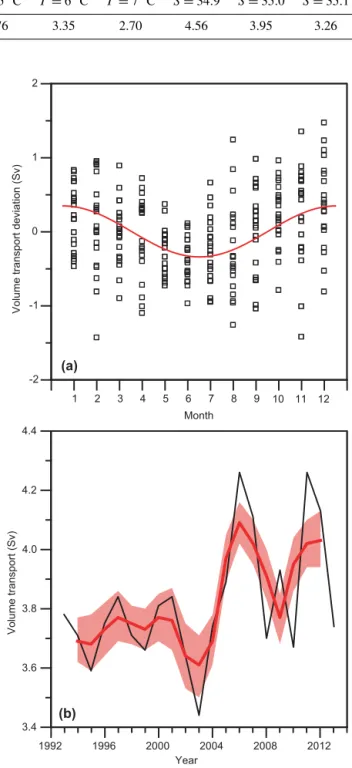
The data set, thus, allows daily estimates of Atlantic wa-ter volume transport, but the algorithms are developed from
Figure 8.Seasonal(a)and interannual(b)variations of Atlantic wa-ter volume transport 1993–2013.(a)Each square represents
trans-port deviation from the 3-year running mean for 1 month. The red curve represents the iteratively determined sinusoidal seasonal fit (Appendix B in the Supplement).(b)Annually averaged transport
regression analyses, that will give better estimates for longer averaging periods. Also, we expect the quality of the altime-try data, and even the validity of geostrophy, to increase with the averaging period. In the following, we therefore will con-sider monthly averaged transport values.
To study the variations in Atlantic water volume transport, monthly averages were calculated for the 1993–2013 period. The overall average was 3.82 Sv and an iterative procedure (Appendix B in the Supplement) was used to extract seasonal (Fig. 8a) and interannual (Fig. 8b) variations. In contrast to previous studies (Hansen et al., 2003, 2010), there is an indi-cation of a seasonal variation with maximum flow around the turn of the year. The maximum correlation coefficient in the fit with the sinusoidal signal was, however, not very high and the seasonal amplitude was below one tenth of the average (Table 3). On average, more than 70 % of the Atlantic water transport occurs between A3and A5(Fig. S5.4.1).
As previously noted (Hansen et al., 2010), the annually averaged Atlantic water volume transport had a minimum in 2003, but since then, it seems to have been at a generally higher level than before 2003 (Fig. 8b). A linear regression on time reveals an increasing trend: 0.016±0.015 Sv yr−1 (Table 3) with a 95 % confidence interval (Sect. 3.6).
3.4 Heat transport
The heat delivered by any inflow branch to the Arctic Mediterranean (Nordic Seas and Arctic Ocean) equals the heat lost by the water before it exits again. Thus, the heat transport is proportional to the temperature of the inflow-ing water minus the temperature of the water when it re-turns back to the Atlantic Ocean either as overflow or as sur-face outflow in the East Greenland Current or through the Canadian Archipelago. Thus, the heat transport of the Faroe Current is only well defined if we know the average outflow temperature, which is the appropriate reference temperature, TRefin Eq. (5). The detailed pathways of the various inflow branches are not well known, but most likely the average outflow temperature of the water that entered in the Faroe Current is close to 0◦C (Hansen et al., 2008). We therefore calculate heat transport relative toTRef=0◦C and term this relative heat transport.
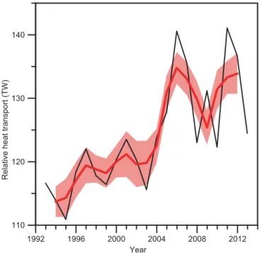
As noted in Sect. 3.2.3, we may simulate daily temperature fieldsTj(z, t )for the whole altimetry period with reasonable accuracy. This allows us to use Eq. (5) to calculate relative heat transport, but it is not obvious that the 4◦C isotherm is the appropriate boundary in this case, since the Atlantic water that by mixing has been cooled below 4◦C originally carried more heat than the Arctic water that has been heated above 4◦C. Instead, we should use a colder isotherm as At-lantic water boundary for heat transport calculation. The cold waters close to the Atlantic water boundary do, however, not transport much heat, especially since average velocities are low. Consistent with that, we also find that the average
rela-Figure 9.Interannual variation of relative (to 0◦C) heat transport 1993–2013. Annually averaged transport (black curve) and 3-year averaged transport (red curve) with the red background representing ±one standard error over each 3-year period.
tive heat transport is not very sensitive to the exact definition of Atlantic water extent (Table S6.1.1).
As for the volume transport, the relative heat trans-port does not exhibit a very pronounced seasonal variation (Fig. S6.1.2), and the seasonal amplitude is about 10 % of the average (Table 3). For the interannual variation, Fig. 9 clearly indicates an increasing trend, which is 1.0±0.5 TW yr−1, from a linear regression on time. This is highly significant and not very dependent on the boundary chosen for Atlantic water extent (Table S6.1.1). Over the 20-year interval from 1993 to 2013, this corresponds to an increase in relative heat transport of∼18 %. Most of the change occurred from 2003 to 2006.
3.5 Salt transport
The salt transport through section N by Atlantic water is given by Eq. (6). Eventually, this salt is returned to the At-lantic by the overflows and surface outflows, but the return-ing water has been diluted by added freshwater and the low-salinity Pacific inflow through the Bering Strait. A rough budget estimate indicates that the salinity is reduced by about 1 on average (Hansen et al., 2008), but the overflows, which will return a large fraction of the Faroe Current, are more saline. The average salinity of the neighboring (Fig. 1a) Faroe Bank Channel overflow is∼34.93 (Hansen and Øster-hus, 2007).
Table 3.Characteristics of transport time series. Averages for the 1993–2013 period. Trends are based on a linear regression of annual
averages on time with 95 % confidence intervals. Seasonal variation is determined by an iterative procedure (Appendix B in the Supplement) where “Rmax” is the maximum correlation coefficient with a sinusoidal seasonal signal, “Ampl.” is the seasonal amplitude and “Max.” is the day number in the year with maximum value.
Seasonal variation
Time series Average Trend Rmax Ampl. Max.
Atlantic water volume transport 3.8±0.5 Sv 0.016±0.015 Sv yr−1 0.34 0.34 Sv 1 Heat transport relative to 0◦C 124±15 TW 1.0±0.5 TW yr−1 0.39 13 TW 307 Absolute salt transport (140±30)×106kg s−1 (1.9±0.7)×106kg s−1yr−1 0.33 14×106kg s−1 14 Salt transport relative to 34.93 (900±140)×103kg s−1 (33±7)×103kg s−1yr−1 0.33 91×103kg s−1 352
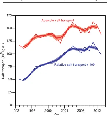
Figure 10.Interannual variation of absolute (red) and relative to 34.93 (blue) salt transport 1993–2013. Annually averaged trans-ports (thin lines) and 3-year averaged transtrans-ports (thick lines) with the background representing±one standard error over each 3-year period. The values for relative salt transport have been multiplied by 100 to fit the same scale as the absolute salt transport.
appropriate to consider the transport relative to some other values for SRef. Using the simulated values forSj(z, t ) in Eq. (8), time series of salt transport for specified values of SRef may be generated, but the problem, again, is to distin-guish between the Atlantic water and other water masses. This introduces considerable uncertainty into calculations of absolute salt transport, but the salt transport relative to higher salinities is much less sensitive to the boundary chosen for Atlantic water extent (Table S6.2.1). This is reflected in the uncertainties for the average values listed in Table 3.
As for volume and relative heat transport, we can ex-tract the seasonal (Table 3) and an interannual variation (Ap-pendix B in the Supplement) from the salt transport time se-ries. This clearly has an increasing trend whether we
con-sider the absolute transport (SRef=0), or the transport rela-tive to 34.93 (Fig. 10). A linear regression of annually aver-aged salt transport on time yields trends that are positive and significantly different from zero for all choices ofSRef (Ta-ble S6.2.1) and more significant, the higher theSRef value. The salt transport relative toSRef=34.93 more than doubled throughout the observational period (Fig. 10).
3.6 Uncertainty estimates
Many different approximations affect the accuracies of the average transport values reported here and fully objective er-ror estimates are difficult to generate from the available in-formation. For all the transport series, the eastward surface velocities, used to calibrate the altimetry data (Fig. 5), are a critical component and their uncertainties will affect all the transport estimates. The uncertainties in extrapolation of ADCP velocities range between 1 and 3 % (Fig. 2). Inter-polating between ADCP sites in the region between A3and A5adds another 1 % to the average eastward surface veloc-ity (Fig. S2.4.4). This region has most of the average trans-port∼3 Sv and we may estimate an uncertainty of∼0.15 Sv for this region. The rest of the section has a smaller average transport∼1 Sv, but with higher relative uncertainties. We add another 0.1 Sv for this part to get a total uncertainty of ∼0.25 Sv from the velocity field. Another uncertainty source for the average volume transport of Atlantic water is the choice of boundary for the Atlantic water extent. From Ta-ble 2, choosing the 3◦C isotherm or the 5◦C isotherm in-stead of the 4◦C isotherm would change the average volume transport of Atlantic water by∼0.25 Sv. Adding this to the uncertainty from the velocity field, we get the value 0.5 Sv.
For the average heat transport, we have to include the 0.25 Sv uncertainty from the velocity field, which is equiv-alent to 7 %, and the uncertainty from the Atlantic water ex-tent is estimated at 3 % (Table S6.1.1). Finally, uncertainty of the Atlantic water temperature (Fig. 7) is assumed to give another 0.15◦C equivalent to 2 %, so that the total adds up to ∼12 % or 15 TW.
assumption of boundary salinity is critical, whereas the un-certainty of Atlantic water salinity becomes more impor-tant with high values forSRef. Combining the various error sources, we estimate an uncertainty of 20 % for absolute salt transport and 15 % for reference salinities close to 34.95.
Most of the uncertainty sources, quoted above, may be seen as biases. Thus, they affect the average transport values, but should not affect the temporal changes in transport appre-ciably. Any remaining errors should be included in the sta-tistical uncertainties cited for the overall trends of transports (Sects. 3.3–3.5). The statistical uncertainties of the trends are the 95 % confidence limits for the slope of the regression line when annually averaged transport values are regressed on the year using the t-distribution. The only exception derives from possible systematic errors in the altimetry data. If these data were to include artificial overall trends, then the trend in vol-ume transport might be affected, but the trends in relative heat and salt transport would still be robust since they are dominated by the trends in Atlantic water temperature and salinity (Fig. 7).
4 Discussion
The transport time series presented in this study are gen-erated from a number of assumptions and approximations: geostrophy, use of the average relative profiles 8k(z) in Eq. (2), our choice of the 4◦C isotherm and 35.0 isohaline as boundaries for Atlantic water extent, etc. Based on an eval-uation of their effects on the results, we find that the chosen method of combining in situ observations with altimetry pro-duces more reliable transport values than estimates based on the in situ data, solely.
We also find that the method allows estimates in periods without in situ velocity measurements as long as there are no major changes in the structure of the velocity field. This justifies the validity of our continuous transport series for the whole altimetry period. One advantage of this is that we now have transport estimates also for the summer months with the ADCPs on land for servicing, especially for June.
4.1 Comparison with other estimates of the IF inflow
The overall average Atlantic water transport for 1993– 2013, estimated in this study (3.8±0.5 Sv) is slightly higher than the previously reported average transport (3.5±0.5 Sv), based on a subset of the same in situ data, but without us-ing altimetry data (Hansen et al., 2003, 2010). The differ-ence is within the uncertainty bounds, however. Comparing monthly averaged volume transport estimates, the best cor-respondence is for the 57 months when all four long-term ADCPs were in operation (Fig. S5.5.1), but even in that case the correlation coefficient is only 0.58 (Table S5.5.1). Con-sidering the approximations made in the old in situ based
es-timates, we conclude, however, that the new transport values should be more realistic than the old ones (Sect. S5.5).
In addition to our own old estimates, there are not many observational transport estimates of the IF inflow, but Rossby and Flagg (2012) have reported estimates based mainly on vessel-mounted ADCP observations from a ferry making regular tracks between Faroes and eastern Iceland. Their val-ues were updated by Childers et al. (2014) who reported an average inflow of 4.6±0.5 Sv across the IFR. Their value is higher than ours, although the uncertainty intervals overlap, but differences in definitions and timing make detailed com-parisons difficult.
Transport values for the IF inflow have also been estimated by ocean models and Sandø et al. (2012) found an average in-flow of 4.7±1.2 Sv using a high-resolution model. The flow over the complicated topography of the IFR remains chal-lenging to model, however, and Olsen et al. (2015) have ar-gued that feedback mechanisms between the IF inflow and the IF overflow make it difficult to disentangle the IF inflow from the net flow across the IFR (IF inflow minus IF over-flow).
4.2 The Faroe Current in a climate perspective
The inflow of Atlantic water to the Nordic Seas plays two main roles in the climate system: (1) it transports heat into the Arctic Mediterranean, which affects sea ice and marine conditions, as well as the climate of the surrounding land masses, and (2) it transports salt into the region, which is a precondition for the thermohaline ventilation and hence the circulation system both locally and more globally through the North Atlantic THC.
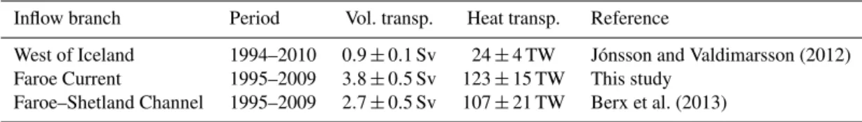
In the literature, the Atlantic inflow is traditionally split into three separate branches (e.g., Østerhus et al., 2005). Based on similar observational period and methodology as ours, average transport values have been reported for the branch west of Iceland (the North Icelandic Irminger Cur-rent) by Jónsson and Valdimarsson (2012) and for the flow through the Faroe–Shetland Channel by Berx et al. (2013). When these values are compared with our results (Table 4), the Faroe Current is found to carry more than 50 % of the total volume transport and 48 % of the total heat transport relative to 0◦C.
This comparison does not take into account the flow of Atlantic water over the shelf region between the Faroe– Shetland Channel and the European continent through var-ious passages including the English Channel. We have no reliable estimate of the combined transports associated with this flow, but the scant observational evidence (Turrell et al., 1990; Childers et al., 2014; Prandle, 1996) indicates that it is well below 1 Sv.
Table 4.Average volume and heat (relative to 0◦C) transport in the three Atlantic inflow branches based on long-term in situ observations.
Inflow branch Period Vol. transp. Heat transp. Reference
West of Iceland 1994–2010 0.9±0.1 Sv 24±4 TW Jónsson and Valdimarsson (2012) Faroe Current 1995–2009 3.8±0.5 Sv 123±15 TW This study
Faroe–Shetland Channel 1995–2009 2.7±0.5 Sv 107±21 TW Berx et al. (2013)
inflow is low, however, and its heat transport does not exceed 20 TW (Woodgate et al., 2012).
The Faroe Current thus remains the dominant inflow branch to the Arctic Mediterranean and its heat transport is likely more than one third of the total oceanic heat im-port to the area. Our observation of an 18 % increase during the 2 decades of observation therefore represents a signifi-cant increase in the total oceanic heat import. The two other branches in Table 4 have also experienced increasing tem-peratures since the mid-1990s (Jónsson and Valdimarsson, 2012; Berx et al., 2013) and it seems likely that their heat transports have increased as well, although the high variabil-ity of the transports of these branches makes statistically sig-nificant trends difficult to identify.
A discussion on the consequences of increased heat trans-port is not within the scope of this paper, but we note that oceanic heat transport has been linked to sea ice reduction in the Barents Sea (Årthun et al., 2012) and north of Svalbard (Onarheim et al., 2014) farther downstream on the path of the Atlantic inflow. In the Arctic Ocean, the submerged Atlantic water is partly isolated from the surface by the halocline, but Rippeth et al. (2015) have demonstrated enhanced vertical mixing over steep topography, allowing more heat from the Atlantic layer to reach the surface. On its way northwards, the heat carried by the Atlantic inflow also tends to warm the ambient waters (Skagseth and Mork, 2012; Mork et al., 2014) and enable pelagic fish species to use a larger part of the Norwegian Sea during the feeding period with huge eco-nomical perspectives (Utne et al., 2012).
The increased heat transport of the Faroe Current stems partly from the increased temperature of the Atlantic wa-ter (Fig. 7) and partly from the increased volume transport (Fig. 8b). The temperature increase mainly occurred from the mid-1990s to 2003, which has been ascribed to a weaken-ing of the subpolar gyre (Häkkinen and Rhines, 2004). As indicated by the inverted gyre index in Fig. 7, the subpo-lar gyre weakened during this period, which allowed warmer and more saline water from more southern areas west of and over the European continental slope to contribute more inten-sively to the Atlantic inflow (Hátún et al., 2005). Later vari-ations in the Atlantic water temperature seem more affected by regional air–sea interaction (Larsen et al., 2012).
The increased volume transport is notable in view of the projected decline of the Atlantic meridional overturning cir-culation (Collins et al., 2013), which is fed by two North At-lantic THC sources, a western (Labrador Sea) and an
east-ern (Arctic Mediterranean) source (Hansen et al., 2004). It has been suggested that the changes observed in the west-ern North Atlantic may indicate a weakening in that THC source (Robson et al., 2014; Rahmstorf et al., 2015). The main branches of the eastern THC component (Nordic Seas – Arctic Ocean) have been monitored since the mid-1990s, but there we find no convincing evidence for a weakening.
The deep branch of the eastern THC component is domi-nated by the two main overflows: through the Denmark Strait and through the Faroe Bank Channel. In the Denmark Strait, Jochumsen et al. (2012, 2015) report no significant overall trend and in the Faroe Bank Channel (Hansen and Øster-hus, 2007, updated with unpublished data), there has been a slightly increasing trend from 1996 to 2014, although not statistically significant.
The picture is very similar for the upper branch. The in-flow branch through the Faroe–Shetland Channel does not show any significant trend (Berx et al., 2013). For the inflow west of Iceland, there are indications of an increasing trend (Jónsson and Valdimarsson, 2012) and Fig. 8b indicates the same for the Faroe Current. It remains to be seen whether these trends will persist.
In this regard, the salt transport is of interest because it may act as a positive feedback on the circulation (Stommel, 1961; Latif et al., 2000). In Table 4, we have not included salt transports; mainly because their values depend critically on the rather ad hoc choice of reference salinity. Regardless of this choice, the salt transport of the Faroe Current has experienced a highly significant increasing trend (Table 3). With reference to the average salinity (34.93) of the Faroe Bank Channel overflow (Hansen and Østerhus, 2007), the salt transport more than doubled from 1993 to 2013 (Fig. 10). The sensitivity of the THC to freshwater anomalies has been widely studied in modeling experiments, but Glessmer et al. (2014) have recently shown that freshwater anomalies in the Nordic seas are mainly of Atlantic, rather than Arctic, origin. This highlights the importance of the salt transport by the Atlantic inflow and the large increase that we have ob-served in the Faroe Current should act to stimulate the over-flows and thereby also the Faroe Current itself (Hansen et al., 2010). Whether this has played any role in the observed strengthening of the Faroe Current (Fig. 8b) remains to be seen.
observed may well be caused by natural processes in the cli-mate system.
5 Conclusions
The method used in this study, combining altimetry and in situ observations, has weaknesses, but is found to give more reliable transport estimates than the previously used method based solely on in situ data. This also allows transport esti-mates for the whole altimetry period, from 1 January 1993, including periods with no in situ current measurements.
Average values for volume and heat (relative to 0◦C) transports of Atlantic water in the Faroe Current were found to be 3.8±0.5 Sv and 124±15 TW, respectively. The aver-age salt transport depends on the choice of reference salinity. All the transports had a seasonal variation with maximum be-tween October and January, although the seasonal amplitudes were only∼10 % of the averages and not very persistent. All the transports also increased during the 1993–2013 period. From the trend analysis, percentage (relative to the begin-ning) annual increases were 0.4±0.4 % yr−1for the volume transport and 0.9±0.4 % yr−1 for heat transport relative to 0◦C. For the absolute salt transport (relative to salinity 0), the annual increase was 2.2±0.8 % yr−1, whereas the salt transport relative to 34.93 increased by 6±1 % yr−1.
The Supplement related to this article is available online at doi:10.5194/os-11-743-2015-supplement.
Acknowledgements. The authors wish to thank captains and
crew on the R/V Magnus Heinason for unfailing support during
measurements at sea. Funding for the in situ measurements has been obtained from the Environmental Research Programme of the Nordic Council of Ministers (NMR) 1993–1998, from national Nordic research councils, from the Danish DANCEA programme, and from the European Framework Programs, lately under grant agreement no. GA212643 (THOR) and under grant agreement no. 308299 (NACLIM). Analysis and preparation of this manuscript was mainly funded by the NACLIM project and by the Danish Strategic Research Program through the NAACOS project.
Edited by: M. Hoppema
References
Årthun, M., Eldevik, T., Smedsrud, L. H., Skagseth, Ø., and Ing-valdsen, R. B.: Quantifying the influence of Atlantic heat on Bar-ents Sea ice variability and retreat, J. Climate, 25, 4736–4743, doi:10.1175/JCLI-D-11-00466.1, 2012.
Berx, B., Hansen, B., Østerhus, S., Larsen, K. M., Sherwin, T., and Jochumsen, K.: Combining in situ measurements and al-timetry to estimate volume, heat and salt transport variability
through the Faroe–Shetland Channel, Ocean Sci., 9, 639–654, doi:10.5194/os-9-639-2013, 2013.
Childers, K. H., Flagg, C. N., and Rossby, T.: Direct veloc-ity observations of volume flux between Iceland and the Shetland Islands, J. Geophys. Res.-Oceans, 119, 5934–5944, doi:10.1002/2014JC009946, 2014.
Collins, M., Knutti, R., Arblaster, J., Dufresne, J.-L., Fichefet, T., Friedlingstein, P., Gao, X., Gutowski, W. J., Johns, T., Krin-ner, G., Shongwe, N., Tebaldi, C., Weaver, A. J., and WehKrin-ner, M.: Long-term climate change: projections, commitments and irre-versibility, Chap. 12, in: Climate Change 2013: the Physical Sci-ence Basis. Contribution of Working Group I to the Fifth Assess-ment Report of the IntergovernAssess-mental Panel on Climate Change, edited by: Stocker, T. F., Qin, D., Plattner, G.-K., Tignor, M., Allen, S. K., Boschung, J., Nauels, A., Xia, Y., Bex, V., and Midgley, P. M., Cambridge University Press, Cambridge, UK, New York, NY, USA, 2013.
Glessmer, M. S., Eldevik, T., Våge, K., Nilsen, J. E. O., and Behrens, E.: Atlantic origin of observed and modelled fresh-water anomalies in the Nordic Seas, Nat. Geosci., 7, 801–805, doi:10.1038/NGEO2259, 2014.
Hansen, B. and Østerhus, S.: Faroe Bank Channel overflow 1995–2005, Prog. Oceanogr., 75, 817–856, doi:10.1016/j.pocean.2007.09.004, 2007.
Hansen, B., Østerhus, S., Hátún, H., Kristiansen, R., and Larsen, K. M. H.: The Iceland–Faroe inflow of Atlantic water to the Nordic Seas, Prog. Oceanogr., 59, 443–474, doi:10.1016/j.pocean.2003.10.003, 2003.
Hansen, B., Østerhus, S., Quadfasel, D., and Turrell, W.: Already the day after tomorrow?, Science, 305, 953–954, 2004. Hansen, B., Østerhus, S., Turrell, W. R., Jónsson, S.,
Valdimars-son, H., Hátún, H., and Olsen, S. M.: The inflow of Atlantic water, heat, and salt to the Nordic Seas across the Greenland– Scotland Ridge, Chap. 1, in: Arctic-Subarctic Ocean Fluxes: Defining the Role of the Northern Seas in Climate, edited by: Dickson, R. R., Meincke, J., and Rhines, P., Springer Science+ Business Media B. V., 15–43, 2008.
Hansen, B., Hátún, H., Kristiansen, R., Olsen, S. M., and Øster-hus, S.: Stability and forcing of the Iceland-Faroe inflow of water, heat, and salt to the Arctic, Ocean Sci., 6, 1013–1026, doi:10.5194/os-6-1013-2010, 2010.
Hátún, H. and McClimans, T. A.: Monitoring the Faroe Current us-ing altimetry and coastal sea-level data, Cont. Shelf Res., 23, 859–868, doi:10.1016/S0278-4343(03)00059-1, 2003.
Hátún, H., Hansen, B., and Haugan, P.: Using an “inverse dynamic method” to determine temperature and salinity fields from ADCP measurements, J. Atmos. Ocean. Tech., 21, 527–534, 2004. Hátún, H., Sandø, A. B., Drange, H., Hansen, B., and
Valdimars-son, H.: Influence of the Atlantic subpolar gyre on the thermoha-line circulation, Science, 309, 1841–1844, 2005.
Häkkinen, S. and Rhines, P. B.: Decline of subpolar North Atlantic circulation during the 1990s, Science, 304, 555–559, 2004. Jakobsen, P. K., Ribergaard, M. H., Quadfasel, D., Schmith, T., and
Hughes, C. W.: Near-surface circulation in the northern North Atlantic as inferred from Lagrangian drifters: variability from the mesoscale to interannual, J. Geophys. Res.-Oceans, 108, 3251, doi:10.1029/2002JC001554, 2003.
se-ries from 1996–2011, J. Geophys. Res.-Oceans, 117, C12003, doi:10.1029/2012JC008244, 2012.
Jochumsen, K., Köllner, M., Quadfasel, D., Dye, S., Rudels, B., and Valdimarsson, H.: On the origin and propagation of Denmark Strait overflow water anomalies in the Irminger Basin, J. Geophys. Res.-Oceans, 120, 1841–1855, doi:10.1002/2014JC010397, 2015.
Jónsson, S. and Valdimarsson, H.: Water mass transport variability to the North Icelandic shelf, 1994–2010, ICES J. Mar. Sci., 69, 809–815, doi:10.1093/icesjms/fss024, 2012.
Larsen, K. M. H., Hátún, H., Hansen, B., and Kristiansen, R.: At-lantic water in the Faroe area: sources and variability, ICES J. Mar. Sci., 69, 802–808, doi:10.1093/icesjms/fss028, 2012. Latif, M., Roeckner, E., Mikolajewicz, U., and Voss, R.:
Tropi-cal stabilization of the thermohaline circulation in a greenhouse warming simulation, J. Climate, 13, 1809–1813, 2000.
Mork, K. A., Skagseth, Ø., Ivshin, V., Ozhigin, V., Hughes, S. L., and Valdimarsson, H.: Advective and atmospheric forced changes in heat and freshwater content in the Norwe-gian Sea, 1951–2010, Geophys. Res. Lett., 41, 6221–6228, doi:10.1002/2014GL061038, 2014.
Olsen, S. M., Hansen, B., Østerhus, S., Quadfasel, D., and Valdimarsson, H.: Biased thermohaline exchanges with the arctic across the Iceland-Faroe Ridge in ocean climate models, Ocean Sci. Discuss., 12, 1471–1510, doi:10.5194/osd-12-1471-2015, 2015.
Onarheim, I. H., Smedsrud, L. H., Ingvaldsen, R. B., and Nilsen, F.: Loss of sea ice during winter north of Svalbard, Tellus A, 66, 23933, doi:10.3402/tellusa.v66.23933, 2014.
Orvik, K. A. and Niiler, P.: Major pathways of Atlantic water in the northern North Atlantic and Nordic Seas toward Arctic, Geo-phys. Res. Lett., 29, 1896, doi:10.1029/2002GL015002, 2002. Østerhus, S., Turrell, W. R., Jónsson, S., and Hansen, B.:
Mea-sured volume, heat, and salt fluxes from the Atlantic to the Arctic Mediterranean, Geophys. Res. Lett., 32, L07603, doi:10.1029/2004GL022188, 2005.
Prandle, D., Ballard, G., Flatt, D., Harrison, A. J., Jones, S. E., Knight, P. J., Loch, S., McManus, J., Player, R., and Tappin, A.: Combining modelling and monitoring to determine fluxes of wa-ter, dissolved and particulate metals through the Dover Strait, Cont. Shelf Res., 16, 237–257, 1996.
Rahmstorf, S., Box, J. E., Feulner, G., Mann, M. E., Robinson, A., Rutherford, S., and Schaffernicht, E. J.: Exceptional twentieth-century slowdown in Atlantic Ocean overturning circulation, Nat. Clim. Change, 5, 475–480, doi:10.1038/nclimate2554, 2015.
Rippeth, T. P., Lincoln, B. J., Lenn, Y.-D., Green, J. A. M., Sund-fjord, A., and Bacon, S.: Tide-mediated warming of Arctic halo-cline by Atlantic heat fluxes over rough topography, Nat. Geosci., 8, 191–194, doi:10.1038/NGEO2350, 2015.
Robson, J., Hodson, D., Hawkins, E., and Sutton, R.: Atlantic over-turning in decline?, Nat. Geosci., 7, 2–3, 2014.
Rossby, T. and Flagg, C. N.: Direct measurement of volume flux in the Faroe–Shetland Channel and over the Iceland–Faroe Ridge, Geophys. Res. Lett., 39, L07602, doi:10.1029/2012GL051269, 2012.
Rossby, T., Prater, M. D., and Søiland, H.: Pathways of inflow and dispersion of warm waters in the Nordic seas, J. Geophys. Res.-Oceans, 114, C04011, doi:10.1029/2008JC005073, 2009. Sandø, A. B., Nilsen, J. E. O., Eldevik, T., and Bentsen, M.:
Mecha-nisms for variable North Atlantic-Nordic seas exchanges, J. Geo-phys. Res.-Oceans, 117, C12006, doi:10.1029/2012JC008177, 2012.
Skagseth, Ø. and Mork, K. A.: Heat content in the Nor-wegian Sea, 1995–2010, ICES J. Mar. Sci., 69, 826–832, doi:10.1093/icesjms/fss026, 2012.
Stommel, H.: Thermohaline convection with two stable regimes of flow, Tellus, 13, 224–230, 1961.
Turrell, W. R., Henderson, E. W., and Slesser, G.: Residual transport within the fair isle current observed during the Autumn Circula-tion Experiment (ACE), Cont. Shelf Res., 10, 521–543, 1990. Utne, K. R., Huse, G., Ottersen, G., Holst, J. C., Zabavnikov, V.,
Jacobsen, J. A., Oskarsson, G. J., and Nøttestad, L.: Horizon-tal distribution and overlap of planktivorous fish stocks in the Norwegian Sea during summers 1995–2006, Mar. Biol. Res., 8, 420–441, 2012.