THE INTEGRATION OF PIGMEAT MARKETS IN THE EU. EVIDENCE FROM A REGULAR MIXED VINE COPULA

doi:10.15414/raae/2016.19.01.03-12

RAAE

REGULAR ARTICLE

THE INTEGRATION OF PIGMEAT MARKETS IN THE EU.

EVIDENCE FROM A REGULAR MIXED VINE COPULA

Vasilis GRIGORIADIS, Christos EMMANOUILIDES, Panos FOUSEKIS *

Address:

Department of Economics, Aristotle University, University Campus, Thessaloniki, Greece 54124 *Corresponding author: fousekis@econ.auth.gr;panosfousekis@gmail.com

ABSTRACT

The objective of this work is to investigate the degree of integration of national pigmeat markets in the EU. This is pursued using monthly wholesale prices from seven major markets and the statistical tool of mixed R-vine copulas. The empirical results suggest that the markets considered do not constitute a great pool in which prices move, boom, and crash together. The markets of Belgium, Germany, and the Netherlands exhibit a higher degree of integration relative to the others, whereas the Italian market exhibits a lower degree of integration. Also, there is an indication that, in certain cases, the benefits of free trade may be unequally distributed between the trading partners.

Keywords: Pigmeat, EU, Price Co-movement, R-Vine Copulas JEL: Q13, C10

INTRODUCTION

Price linkages in the physical or in the product space have long attracted the attention of economists and policy makers. The interest is grounded in the recognition that the strength and the pattern of price relationships may provide information on whether a given set of spatial markets are integrated or segmented. In well integrated spatial markets prices tend to co-move. This means that a price shock in one market stimulates responses in the other markets. In the long-run, shocks are fully transmitted and the price difference of a homogeneous commodity between any two geographically separated markets becomes (at most) equal to the trade-related transaction costs (weak version of the Law of One Price - LOP). Under segmentation, however, profitability opportunities are not fully exploited and the result is a loss in economic efficiency (Emmanouilides and Fousekis, 2012; Reboredo, 2011; Serra et al., 2006; Asche et al., 1999).

Several empirical works on the integration of spatial primary commodity markets have focused on the national (geographically separated) markets of the European Union (EU) (e.g. Emmanouilides et al., 2014; Emmanouilides and Fousekis, 2012; Serra et al., 2006). This has not been accidental. The establishment of a large European market has been the central policy goal of the EU over the last 30 years. Nevertheless, survey-based evidence from super markets around Europe suggests that considerable and persistent price differences for virtually identical food commodities still exist even between neighbouring or comparable member states (European Commission, 2013a and 2013b).

Against this background, the objective of the present work is to assess the integration of the EU pigmeat markets. This is pursued using monthly data from seven major players in the intra-EU trade of pigmeat over 1995 to 2015 and the recently developed statistical tool of a

mixed R-vine copula (where R stands for Regular). Copulas are considered to be very suitable for analysing co-movement between stochastic processes (such as prices in space) because they allow the joint behaviour of these processes to be modelled independently of their marginal behaviour; they dispense with the need to assume that marginal distributions belong to the same family; they are capable of capturing not only linear but also non-linear co-movement; and they provide information both about the degree and the structure of co-movement (Patton, 2013 and 2012; Nelsen, 2006; Fermanian and Scaillet, 2004).

Recent applications of copulas in the analysis of price interrelationships are those by Reboredo (2011) who investigated price co-movement in four regional oil markets, by Serra and Gill (2012) who assessed price linkages between biodiesel, diesel, and crude oil prices in Spain, by Emmanouilides et al. (2014) who examined price co-movement in principal EU olive oil markets, by Emmanoulides and Fousekis (2015) and Panagiotou and Stavrakoudis (2015) who investigated price transmission along the meat supply chain in the USA.

The overwhelming majority of copula-based empirical works on co-movement (including those cited above) have analysed simple bivariate stochastic processes. This is a limitation because multidimensional models are far more appropriate than bivariate ones for the assessment of spatial market integration (e.g. Goodwin and Ortalo-Magne, 1992). The works of Joe (1996 and 1997), Bedford and Cooke (2001), Aas et al. (2009), and

(2015) employed copula vines to investigate housing price linkages in four US regions, and Chi and Goodwin (2011) also relied on copula vines to analyse relationships between corn prices in five North Carolina regions. The use of a mixed R-vine here is expected to provide new insights about the ways EU national pigmeat markets are related to each other and, in turn, about the success of the long-standing efforts to integrate them into a single large European market.

The structure of the present work is as follows: the next section contains the analytical framework, that is, presentation of two-dimensional copulas and their extension to high-dimensional ones and to R-vines. This is followed by the section that presents the data, the empirical models and the empirical results (identification of the appropriate R-vine structure for seven major EU markets, assessment of the strength and the pattern of price co-movement). The last section offers conclusions.

DATA AND METHODS

ANALYTICAL FRAMEWORK

Two-Dimensional Copulas

The use of copulas to assess dependence among stochastic processes has its roots in Sklar’s (1959) Theorem according to which a d-dimensional joint distribution function can be decomposed into its d univariate marginal distributions and a joining function known as copula. In the simplest case with d=2, let ( ,Y Y_{1 2}) be a bivariate stochastic process with joint distribution function

1 2

( , )

F y y and marginal distribution functions F y₁( )₁ and

2( 2)

F y , respectively. Consistency with uppercase for

Sklar’s Theorem

1 2 1 1 2 2

( , ) { ( ), ( )}

F y y C F y F y (1)

where C is the copula function. Provided that marginal distribution functions are continuous, C, F1, and F2 are

completely determined by F y y( ,_{1 2}). The converse of

Sklar’s theorem also holds meaning that for any pair

1 2

(F F, ) and for any copula function C, the function F given in (Eq. 1) defines a valid joint distribution with marginals F1 and F2.

The copula C is a bivariate distribution function with uniform margins and it can be obtained from (Eq. 1) as Eq. 2.

1 1

1 2 1 1 2 2

( , ) ( ( ), ( ))

C u u F F y F y (2)

with 1

i

F and u_i (i1, 2) being marginal quantile functions and uniformly distributed random variables on [0, 1], respectively. The copula density function is given by Eq. 3.

1 1

2

1 1 2 2

1 2 1 1

1 2 1 1 1 2 2 2

( ( ), ( )) ( , )

( ( )) ( ( )) f F u F u C

c u u

u u f F u f F u

 

 



  

 

1 2

1 1 2 2

( , ) ( ) ( ) f y y f y f y

 (3)

where f is the joint density function associated with F, and f₁ and f₂ are the marginal density functions of Y₁ and

2

Y , respectively. From (Eq. 3) it follows that

1 2 1 1 2 2 1 1 2 2

( , ) ( ( ), ( )) ( ) ( )

f y y c F y F y f y f y (4)

suggesting that the density function f (Eq. 4) can be expressed as the product of the copula density functionc and the marginal density functions f₁ and f₂.

A standard measure of overall co-movement between

two stochastic processes is Kendall’s τ, that reflects the difference between the probability of concordance and the probability of discordance for two independent pairs of observations drawn from the joint distribution of Y1 and Y2. Given a copula function C, it is calculated as Eq. 5.

2 1 2

[0,1] 1 2

1 4 C Cdu du u u

    

 



(5)

and it ranges from +1 (perfect concordance) to -1 (perfect discordance) (e.g. Genest and Favre, 2007; Nelsen, 2006).

Co-movement at the tails of the joint distribution is assessed by the lower and the upper tail coefficients. The lower tail coefficient is defined as Eq. 6.



1 2



0 0

( , )

lim lim

L u u

C u u Pr U u U u

u

  _    _ (6)

and measures the probability that Y₁ is below a low quantile, given that Y₂ is also below that low quantile. The upper tail coefficient is defined as Eq. 7.



1 2



1 1

1 2 ( , )

lim lim

1

U u u

u C u u Pr U u U u

u

 _ _

 

   

 (7)

and measures the probability that Y₁ is above a high quantile, given that Y₂ is also above that high quantile. In short, the two tail co-movement coefficients provide information about the likelihood for the two stochastic processes to crash and to boom together, respectively (e.g. Reboredo, 2011).

Higher-Dimensional Copulas and R-vines

The application of copula models to multivariate stochastic process has been, until very recently, hindered

by a “curse of dimensionality” problem. Specifically,

copula models other than the Gaussian or the t-copula do not readily extend to d>2 dimensions, while a number of attempts to generalize Archimedean copulas involved the imposition of unrealistic assumptions (parameter restrictions) and/or presented serious difficulties when applied to data (e.g. Hofert, 2011; Savu and Trede, 2010; Joe, 1997).

conditional copula densities (called pair-copulas). As a starting point consider a 3-dimensional stochastic process with density f y y( 1, 2,y3). A possible decomposition of

f is Eq. 8.

1 2 3 1 1 2 1 3 1 2

( , , ) ( ) ( | ) ( | , )

f y y y  f y f y y f y y y . (8)

Using Sklar’s Theorem (Eq. 9),

1, 2 12 1 1 2 2 1 1 2 2

2 1

1 1 1 1

( ) ( ( ), ( )) ( ) ( ) ( | )

( ) ( )

f y y c F y F y f y f y f y y

f y f y

  

12( 1( 1), 2( 2)) 2( 2)

c F y F y f y

 (9)

and (Eq. 10)

2, 3 1

3 1 2 23|1 2 1 3 1

2 1

( | y )

( | , y ) ( ( | y ), ( | y ))

( | y ) f y y

f y y c F y F y

f y

 

13( 1(y ),1 3( 3)) 3( 3)

c F F y f y . (10)

Substituting (Eq. 9) and (Eq. 10) into (Eq. 8) one observes that the 3-variate joint density function is just the product of the three marginal densities f i_i( 1, 2,3), the two unconditional pair-copula densities c₁₂ and c₁₃, and

the conditional pair-copula

c

23|1

.

The marginal

conditional distribution functions (transformed variables)

1

( _j| ), 2, 3

F y y j entering in (Eq. 10) can be calculated

as

1 1 1

1

1 1

( ( ), ( )) ( | )

( )

j j j

j

C F y F y F y y

F y 



 (Zimmer, 2015; Aas

et al., 2009).

Any d-dimensional process may be expressed as the product of marginal densities, unconditional pair-copula densities, and conditional pair-copula densities. The decomposition, however, is not unique. To see it notice that f y y( ₁, ₂,y₃) f₃(y₃) (f y₂|y₃) (f y₁|y₂,y₃) is another perfectly valid factorization instead of that shown in (8). As a matter of fact, the number of possible factorizations grows exponentially with d. Because of this, the details of a particular factorization are represented by a graph theoretical construction, termed as regular vine (R-vine). In the following we present a simple example of a regular vine with a small number of dimensions. Exhaustive and highly technical treatments can be found in Dißmann et al. (2013), Aas et al. (2009), and Bedford and Cooke (2001).

Consider now a 5-dimensional stochastic process,

1 2 3 4 5

( , , , , )

y y y y y y . An R-vine for that process is a sequence of linked/nested trees (Figure 1). In that Figure, Tree 1 consists of unconditional pair copulas only. These are c12, c23, c34 and c35 for the unconditional pairs of

stochastic processes (y y₁, ₂), (y₂,y₃), (y y₃, ₄), and

3 5

(y y, ), respectively. Tree 2 involves bivariate copulas conditioned on a single stochastic process only. Drawing on the information available in Tree 1, these are

1,3|2

,

2,4|3

,

c

c

and

c

25|3 for the conditional pairs of

stochastic processes (y y₁, ₃|y₂), (y₂,y₄|y₃), and

2 5 3

(y ,y |y ), respectively. Tree 3 involves bivariate copulas conditioned on two stochastic processes. Drawing on information available in Tree 2, these are

c

1,4|23 and

4,5|23

c

for the conditional pairs of stochastic processes

1 4 2 3

(y y, |y , y ) and (y₄,y₅|y₂, y )₃ , respectively. Finally, Tree 4 involves a bivariate copula conditional on three stochastic processes. Drawing on the information available in Tree 3, this is

c

1,5|234 for the conditional

stochastic process ( ,y y_{1 5}|y₂, y , y )_{3 4} . The factorization of the joint density function of the 5-dimensional stochastic process is

1 2 3 4 5(12 23 34 35) (1,3|2 2,4|3 2,5|3) (1,4|23 4,5|23) (1,5|234)

f         f f f f f c c c c c c c c c c (11)

Extensions to processes with arbitrary dimensions can be achieved along the same lines with the required conditional marginal distribution functions being calculated recursively moving down an R-vine tree.

The empirical application of an R-vine requires (Dißmann et al., 2013; Czado and Aas, 2013):

(a) determination of the vine’s structure (i.e. selection of

the unconditional and conditional bivariate copulas); (b) selection of the most suitable parametric family for

each bivariate copula; and

(c) estimation of the selected bivariate copula families. To determine the appropriate structure (factorization) for a given data set Dißmann et al. (2013) proposed a sequential top-down approach (algorithm). This involves selecting successively Tree 1, Tree 2, and continue to Tree d-1. Each tree is selected in such as a way as to be the maximal spanning one, that is, the tree achieving the strongest pair-wise dependencies, as measured by the sum

of absolute empirical Kendall’s tau. Technical details and the rationale behind the sequential approach are available in Dißmann et al. (2013). Alternative heuristic algorithms of similar spirit are available in the literature (e.g. Kurowicka, 2011; Brechmann, 2013). Given the R

-vine’s structure, the most suitable bivariate copula

families (including the independence copula) are chosen using an appropriate goodness-of-fit criterion. Given the best copula family for a given pair of stochastic processes (conditional or unconditional), the copula’s parameters are estimated by employing an appropriate statistical method. Finally, the sequential parameter estimates of the individual pair-copulas are used as starting values for estimating the R-vine in a single step via Maximum Likelihood.

Figure 1. A Hypothetical R-vine with five stochastic processes

A piece of information which cannot be obtained through standard bivariate modelling concerns the so called central markets. A market may be viewed as a central one when it has direct linkages with at least two other markets. With reference to tree 1 (Figure 1), markets number 3 and number 2 are central. The prices in central markets are the conditioning stochastic processes for the construction of Tree 2 (this is how trees are linked). Moreover, an R-vine may provide information about possible clustering of markets. A cluster may be viewed as set of markets which are directly connected to the same central market and they have certain common characteristics such as the strength and the pattern of co-movement.

Conditioning on a third stochastic process plays an important role in assessing the degree of pure co-movement between two other processes. It is well known that the influence of a third variable may either make co-movement between two other variables to appear stronger or it may cloud it; that is why conditional measures of co-movement are often computed and presented in empirical economic studies (e.g. Aguirar-Conraria and Soares, 2014). If one finds that after controlling for a third price, co-movement between two other prices decreases she (he) may conclude that their interdependence was due to the third price; if the opposite happens, she (he) may conclude that the third price was clouding their relationship. It appears, therefore, that an R-vine is capable of revealing aspects of co-movement that bivariate modelling is not. Because price changes in geographically separated markets for the same commodity typically exhibit a

positive association, one expects co-movement to become weaker with conditioning (Dißmann et al., 2013). Therefore, higher numbered trees often become redundant as they consist of pairs of stochastic process the dependence of which can be best described by the independence copula.

DATA, EMPIRICAL MODELS, AND EMPIRICAL RESULTS

The data for the empirical analysis are monthly wholesale prices (in Euros per 100 kg) for the period 1995:1 to 2015:5. They have been obtained from the European Commission and they come from seven major pigmeat producing countries: Belgium (BE), Germany (DE), Denmark (DK), Spain (ES), France (FR), Italy (IT), and the Netherlands (NL). These countries account for more than 75% of the total pigmeat production in EU-28 (and for more than 85% in EU-15). Table 1 presents the respective production shares in EU-28 for the year 2013. Another important pigmeat producer is Poland, with a share of 7.7%. However, it is not considered here because monthly data from that country are available only after 2006. There are trade flows between them both in terms of fresh and frozen pigmeat and in terms of live animals (weaners, breeders, and slaughter pigs) and processed pigmeat (bacon, ham, etc.). The existence of trade flows is a necessary condition for the smooth transmission of price shocks from one national/spatial market to another. To assess the degree and the structure of price co-movement

1 2 3

4

5

Tree 1

1,2 _{2, 3}

3, 4

3, 5

Tree 2

1, 3|2 2, 4|3 2,5 |3 Tree 3

1,4 |23 4, 5|23 Tree 4

1,2 2,3

3,4

3,5

1,3|2

2,4|3

2,5|3

1, 4|23 4, 5|23

we follow earlier empirical works on the topic (e.g. Emmanouilides and Fousekis, 2015; Emmanoulides et al. 2014; Serra and Gil, 2012; Reboredo, 2012; and Reboredo, 2011) by applying parametric copula families to the rates of price change (i.e. to the price shocks) calculated as dlnp_it, where p_it is the price of pigmeat in market i= BE,DE,DK,ES,FR,IT, and the NL at time t.

Table 1. Pig Meat Production Shares (2013) in EU-28 * Country Share (%) Country Share (%)

BE 5.2 FR 8.8

DE 25 IT 7.4

DK 7.2 NL 6

ES 15.6 * _{Eurostat (2014).}

The asymptotic properties of the different copula estimators have been established for i.i.d. observations (e.g. Patton, 2013 and 2012; Rémillard, 2010). Time series data, however, may exhibit autocorrelation and/or time-varying volatility (ARCH) effects. To account for this potential problem, as in Emmanouilides and Fousekis (2015), Serra and Gil (2012), and Czado, et al. (2012), we have fitted appropriate ARMA-GARCH models to the individual time series of raw rates of price change. Table 2 presents the p-values from the application of the Box-Pierce and the ARCH-LM tests to the resulting standardized innovations (filtered data), at various lag lengths. Details on the estimated ARMA-GARCH models are available upon request. The filtered data are free from autocorrelation and ARCH effects.

Table 2. p-values of the Tests for Autocorrelation and for ARCH Effects

Filtered Rates

of Price Change

Box-Pierce ARCH-LM No of Lags No of Lags

1 6 12 1 6 12

BE 0.78 0.88 0.09 0.67 0.06 0.4 DE 0.53 0.87 0.22 0.35 0.24 0.62 DK 0.31 0.87 0.86 0.12 0.36 0.44 ES 0.66 0.89 0.98 0.76 0.41 0.27 FR 0.87 0.95 0.6 0.87 0.99 0.96 IT 0.95 0.76 0.88 0.67 0.72 0.31 NL 0.91 0.94 0.49 0.82 0.27 0.54

Source: Authors’ estimations

Table 3 presents the pairwise empirical Kendall’s τ, denoted as



ˆi j

, as well as the sum ,

,

ˆi j j j i







as a measure of the degree of interdependence between a given market

i and all the remaining markets taken together (Brechmann and Schepsmeier, 2013; Czado et al., 2012). The empirical value of Kendall’s tau is calculated

as





2 n n

n P Q  _{ }

 , where n is the number of observations

and Pn (Qn) is the number of concordant (discordant) pairs. There are three markets (DE, NL, and BE) where the filtered rates of prices changes which, exhibit high degrees of overall co-movement with each other and considerable degrees of overall co-movement with the majority of the remaining. Germany is the largest producer of pigmeat and its people consume more pigmeat than those in other

member states. In addition, it is the one of the world’s

leading exporters and a significant importer. As such is has a big influence in pigmeat markets throughout Europe. Belgium and the Netherlands despite their small size, are leading pigmeat exporters directing their production surplus primarily within the EU. The high values of

Kendall’s τ between NL, BE, and DE implies that producers in the Netherlands and in Belgium track price developments in each other as well as in Germany which is, by far, the most important outlet of their exports. The filtered rates of price change in France show their highest degrees of co-movement with those of its close neighbours (DE,BE, ES, and NL); the filtered rates of price change in Spain exhibit their highest degrees of co-movement with those in FR, DE, BE, and NL. Denmark shares common characteristics with BE and NL (i.e., it is a small country with a high degree of self-sufficiency and a leading exporter in intra EU pigmeat trade for fresh and frozen meat and for live animals). It is, therefore, somehow

surprising that the pairwise empirical Kendall’s τ for Demark are relatively small. The same observation (but to a larger degree) applies to Italy as well since Italy is the largest net importer of pigmeat in the EU and, thus, a key market for many exporting member states.

On the basis of the sum of the absolute values of the

pairwise Kendall’s τ, the German market shows the highest degree of interdependence with all the remaining (3.03) followed closely by the Netherlands, and Belgium. France, Spain and Denmark (in this order) show similar degrees of interdependence, while Italy shows the lowest by far.

Table 3. Empirical Kendall’s τ for the Filtered Data

Country BE DE DK ES FR IT NL , ,

ˆi j j j i







BE 1 0.72 0.37 0.41 0.46 0.25 0.71 2.91

DE 1 0.39 0.43 0.46 0.25 0.79 3.03

DK 1 0.36 0.38 0.25 0.39 2.12

ES 1 0.46 0.23 0.41 2.29

FR 1 0.33 0.44 2.52

IT 1 0.26 1.57

NL 1 2.99

The flexibility of mixed R-vines lies in the fact that they allow each pair-copula family in the factorization of the multivariate copula density to be chosen independently from the rest. Here to allow for a variety of possible co-movement patterns, we have considered for each pair-copula a number of alternative pair-copula families and we have selected among them the one that best fits the data. The 10 families are the Gaussian, the Student–t, the Clayton, the Gumbel, the Frank, the Joe, the Clayton-Gumbel, the Joe-Clayton-Gumbel, the Joe-Clayton, and the Frank-Joe, which are commonly used in Economics and Finance.

Given that a copula is a distribution function with uniform margins on [0,1], for the empirical application we have converted each of the filtered rates of price change into the so called copula data (i.e. data on [0,1]) using the empirical probability integral transformation and a scaling factor equal to n n/ 1 (e.g. see Emmanouilides and Fousekis, 2015; Serra and Gil, 2012; Czado et al., 2012). To establish that each copula data series is indeed drawn from the uniform distribution on [0,1] we employed the non-parametric Kolmogorov-Smirnov (KS) test. Table 4 presents the results. In all cases, the null hypothesis that the empirical distribution is consistent with the uniform distribution on [0,1] cannot be rejected at any reasonable level of significance. Thus, we conclude that the copula data can be safely used to estimate the components of the mixed R-vine. For the selection of the most suitable pair-copulas we have used the AIC information criterion, shown to perform very well in this context (e.g. Dißmann

et al., 2013; Brechmann, 2010; Manner, 2007).

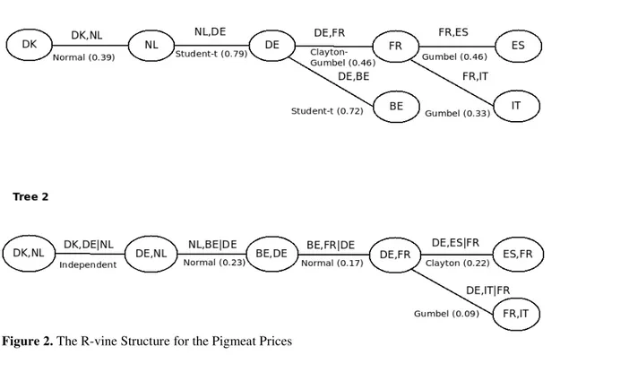
Figure 2 presents the empirically determined R-vine structure for our data, its individual components (i.e. unconditional and conditional pair-copulas), and the

empirical value of Kendall’s τ for each pair of the stochastic processes modeled. The selection of the R-vine structure and its components along with all estimations

and testing have been carried out using package VineCopula in R by Schepsmeier, U. et al. (2015). Note that although for seven stochastic processes the dependence structure may be represented with an R-vine consisting of a maximum of six trees, in our application the actual number of trees turned out to be just two. The reason is that after conditioning with more than one stochastic processes, the resulting transformed variables have become independent from each other, rendering the trees lower in the vine redundant. Independence has been

tested using the statistic









9 1

ˆ

2 2 5

n n T

n





 

 , where n is

the number of observations and ˆ is the empirical value

of Kendall’s tau. The statistic, under the null of

independence, follows the N(0,1) distribution (e.g. Brechmann and Schepsmeier, 2013).

Table 4. Results from the Application of the KS Test on the Copula Data

Country Empirical Value of the KS Statistic * BE 0.067 (0.578) DE 0.054 (0.84) DK 0.063 (0.656) ES 0.03 (0.999) FR 0.072 (0.487) IT 0.043 (0.963) NL 0.039 (0.989)

* Calculated as sup |x F xn( )F x( ) |where x is the data set, Fn is

the empirical distributionand F is the test (null) distribution, here

the Uniform [0,1]; p-values are shown in parentheses.

Source: Authors’ estimations

Tree 1 is the maximal spanning tree for the unconditional univariate stochastic processes modelled. Therefore, the values of the bivariate measures of

dependence (Kendall’s τ) appearing in Tree 1 are exactly the same as their counterparts reported in Table 3. The tree indicates that there are three potential central markets, namely, Germany, France, and the Netherlands; DE is connected directly to BE, FR, and the NL; FR is connected directly to DE, ES, and IT, whereas NL is connected directly to DE and DK. It appears as if the pair of markets (France, Germany) is the channel through which price shocks in Belgium, Denmark, and in the Netherlands are associated with those in Italy and in Spain.

The best fitting copula family for the pairs (DE,NL), and (DE,BE) is the two-parameter Student-t. This particular copula is consistent with symmetric tail co-movement suggesting that extreme positive and extreme negative price shocks are likely to be transmitted from one spatial market to the other with exactly the same intensity. The best fitting copula family for the pair (DE,FR) is two-parameter Gumbel- Clayton consistent with potentially asymmetric co-movement at the two extremes. The best fitting copula family for the pairs (FR,IT) and (ES,FR) is the one-parameter Gumbel which is consistent with upper tail co-movement only. Finally, the best-fitting copula family for the pair (NL, DK) is the one-parameter Gaussian which is consistent with zero tail co-movement at the extremes.

Tree 2 is the maximal spanning tree for the conditional stochastic processes. One observes that the degrees of overall co-movement are far lower compared to those for the unconditional ones, reported in Table 3. This is in line with the relevant discussion in the Analytical Framework.

For the pair (DE|NL, DK|NL), in particular, Kendall’s τ dropped from 0.39 to 0 suggesting that co-movement of prices between DK and DE is completely explained by price changes in Netherlands. Co-movement for the pair (BE|DE, NL|DE) is best described by the Gaussian copula, for the pair (DE|FR, ES|FR) by the Clayton copula which consistent with lower tail co-movement only, for the pair (BE|DE,FR|DE) by the Gausssian, and for the pair (DE|FR,IT|FR) is best described by the Gumbel copula.

Table 5 presents parameter estimates along with their respective standard errors for the unconditional and the conditional pair-copulas making up the R-vine structure. In all cases the parameter estimates are statistically significant at 5 percent level (or less). Table 6 presents the point estimates and standard errors of the tail co-movement coefficients. Their standard errors have been obtained using the block bootstrap approach of Politis and Romano (1994). We note that exactly the same approach has been employed in the earlier works of Emmanouilides and Fousekis (2015), and Patton (2012 and 2013). The block length for each pair has been determined optimally as suggested by Patton, Politis and White (2009). All are statistically significant at the 5 percent level (or less). The magnitude of the tail coefficients is in line with that of the corresponding overall measures of co-movement. For example, the tail coefficients receive their highest values for the pairs (DE,NL), (DE,BE), and (ES,FR) and the lowest for the pair (DE|FR,IT|FR). Also, the difference between the two

tail coefficients for the pair (DE,FR) is statistically insignificant suggesting that extreme positive and extreme negative shocks between the German and the French markets are likely to be transmitted symmetrically (that is, with the same intensity).

The empirical finding that the pairs (DE, NL) and (DE, BE) exhibit by far the highest degrees of overall co-movement (ˆ0.7) and that the co-movement structure between price shocks in both the Netherlands and in Belgium on the one hand and in the central market (Germany) on the other is best captured by the symmetric Student-t copula, provides a strong indication that BE, DE, and NL is a potential cluster of markets. As already mentioned, NL and BE export primarily in DE and they follow closely the price developments in it. Also, NL, BE, and DE share borders with each other and all lie in the heart of the main pigmeat production basin of the EU which extends from North-West France (Bretagne) to Denmark. The result for DE, the NL, and BE, makes perfect sense and appears to offer support for the method employed here.

Table 5 One Step Maximum Likelihood Estimation Results for the R-vine

Pairs of Stochastic Processes

Copula Model

Parameters*

DK,NL Normal

=0.586 (0.037)

DE,NL Student-t

=0.943 (0.007)

=4.26 (1.41)

BE,DE Student-t

=0.899 (0.013)

=3.19 (0.856)

ES,FR Gumbel

=1.78 (0.089)

DE,FR

Clayton-Gumbel =0.499 (0.143)

=1.422 (0.098)

FR,IT Gumbel

=1.473 (0.073)

NL|DE, BE|DE Normal

=0.339 (0.056)

BE|DE, FR|DE Normal

=0.201 (0.059)

DE|FR, ES|FR Clayton

= 0.512 (0.112)

DE|FR, IT|FR Gumblel

= 1.08 (0.046) Source: Authors’ estimations

Extreme positive and extreme negative shocks are transmitted symmetrically between FR and DE as well. In this respect, the structure of price co-movement for the pair (DE,FR) is similar to those for the pairs (DE,NL) and (DE,BE). The degree of overall price co-movement, however, between FR and the other three markets is relatively low (ˆ0.5). Therefore, the empirical evidence that France is a part of the same cluster with DE, BE, and the NL is somehow weaker. Denmark is even more unlikely to belong to the same cluster with DE, BE, and the NL both because of the relatively low degree of overall co-movement (ˆ0.4) as well as because of the different

1

ˆ



1

ˆ



2

ˆ



1

ˆ



2

ˆ



1

ˆ



1

ˆ



2

ˆ



1

ˆ



1

ˆ



1

ˆ



1

ˆ



1

ˆ

co-movement structure (Gaussian instead of Student-t copula). This may be an indication that it takes more than 1 month for price shocks to transmit it between DK and the rest of the countries. Finally, Tree 1 points to another possibility, that is, a market cluster consisting of France, Italy and Spain especially because the price co-movement structures between France (the central market) on the one hand and Italy and Spain on the other are identical (best captured by the Gumbel copula). It should be noted, however, that asymmetric price co-movement implies a low degree of market integration (e.g. Emmanouilides et al. 2014; Reboredo, 2011).

Table 6. Tail Dependence Coefficients

Countries Copula Tail Dependence DE,NL Student-t



L



U 0.715 (0.058)

BE,DE Student-t



L



U 0.661 (0.052)

ES,FR Gumbel



U 0.529 (0.029)

DE,FR Clayton-Gumbel

0.43 (0.099) L

 

0.36 (0.066)

U





FR,IT Gumbel



U 0.4 (0.034)

DE|FR,

ES|FR Clayton



L0.256 (0.086)

DE|FR,

IT|FR Gumbel



U 0.099 (0.046) Source: Authors’ estimations

DISCUSSION AND CONCLUSIONS

The objective of this work has been to assess the integration of the EU pigmeat markets. This has been pursued using monthly data from seven major players in the intra-EU pigmeat trade and the recently developed tool of a mixed R-vine copula. The empirical copula-based assessment of market integration utilizes information on both the strength as well as on structure of price movement. In particular, a high degree of overall price co-movement together with a symmetric and a strictly positive co-movement at the extremes of the joint distribution are considered to be indicators of well integrated markets.

The analysis here revealed that substantial differences exist with respect to the above indicators among the unconditional pairs of price shocks examined. The degrees of overall co-movement vary widely while the best fitting copula families range from the Gaussian (consistent with zero co-movement at the extremes) to Gumbel (consistent with co-movement at the upper extreme only). Similar too are the observations for the conditional pairs of price shocks.

The empirical results, therefore, suggest that the markets of the seven major players in the intra-EU pigmeat trade do not constitute a great pool in which prices move, boom, and crash together. Germany, Belgium, the Netherlands, and to a lesser extent France is a potential cluster where the strength and the pattern of price co-movement between the central market (Germany) and the rest are generally the ones expected for well integrated markets. France, Italy, and Spain constitute another potential cluster with markets, however, they are not well

integrated with each other. Denmark does not fit well in any of the two potential market clusters.

Physical proximity and intensity of trade flows only partly explain the empirical finding of market segmentation (regionalization). Belgium, Germany, and the Netherlands share borders and have intense trade relations. The same is true for France and Spain. In the last case, however, extreme negative shocks are not transmitted from one market to the other.

Asymmetric price co-movement in international trade of primary commodities is typically attributed to possession of local market power, asymmetric transaction costs, consumer preferences for specific attributes of domestically produced goods (real or perceived quality differentiation), and differences in information available between hub and spoke markets (Ghoshray, 2009; Meyer and von Cramon Taubadel, 2004).

With respect to the possession of market power, pig slaughtering in the EU has been concentrated in the hands of few abattoirs; just 5 of them conduct 65% of pig slaughtering in the EU-28 (Brossard and Montage, 2012). The activities of the big abattoirs, most of the time are not restricted to a single member state. For example, VION (with a share of 19.3%) has its activities in both the

Netherlands and Germany while Tönnies Fleisch (with a

share of 13%) has its activities in both Denmark and Germany. The operation of the big slaughtering firms in the main production basin of the EU, however, does not appear to have been an impediment to symmetric price co-movement in the German, Dutch, Belgian, and French markets.

Asymmetric transaction costs are thought to arise due to the use of non tradable inputs (i.e. inputs, whose prices are determined by national factors rather than by international competition) and to the existence of transportation infrastructure or handling facilities tailored to unilateral trade (e.g. tailored to importing rather than to exporting) (Goodwin and Piggott, 2001). Differences in labour relations (e.g. payments, social security contributions, working schedules) are still prevailing even among the oldest member states of the EU-28. The same holds for taxes applied to services or to production processes.

With regard to the direction of trade, it is primarily unilateral for the panel of markets examined. For example, France is by far a net importer in its relationship with Spain, Italy is a net importer in its relationship with the other six countries, while Belgium and Netherlands are net exporters in their relationship with Germany. Nevertheless, asymmetric co-movement is relevant only for the pairs of markets (France, Spain) and (France, Italy).

Asymmetric price co-movement has implications on the distribution of benefits between trading partners. For example, consumers in France are likely to be hurt by price booms but they are not likely to benefit from price crashes in the exporting country (Spain). Similarly, consumers in Italy are likely to feel extreme positive shocks in France but they are not likely to gain from extreme negative shocks in the same country.

To the best of our knowledge there have been only two earlier works that relied on copulas (bivariate or vine) to investigate spatial price linkages for agricultural commodities. Chi and Goodwin (2011) found that price co-movement in North Carolina regions was best described by Gaussian and/or Frank copulas (both consistent with zero co-movement at the extremes). Emmanouilides et al. (2014) in their study on price relationships in the principal EU olive markets reported low degrees of overall movement and asymmetric co-movement at the extremes for the two biggest markets (Spain and Italy).

The evidence of segmentation obtained here probably implies that removing all trade barriers may be only a necessary but not a sufficient condition for integrating the national EU agricultural markets. Of course, this requires additional empirical substantiation. Further work on the topic is certainly warranted.

REFERENCES

AAS, K., CZADO, C., FRIGESSI, A., BAKKEN, H. (2009): Pair-copula Constructions of Multiple Dependence. Insurance: Mathematics and Economics, 44(2), p. 182-198.

doi

:

_{10.1016/j.insmatheco.2007.02.001}

AGUIRAR-CONRARIA, L., SOARES, M. (2014): The Continuous Wavelet Transform: Moving Beyond Univariate and Bivariate Analysis. Journal of Economic Surveys, 28(2), p. 344-375. doi: 10.1111/joes.12012 ASCHE, F., BREMNES, H., WESSELS, C. (1999): Product Aggregation, Market Integration, and Relationships between Prices. American Journal of Agricultural Economics, 81(3), p. 568-581.

doi: 10.2307/1244016

BEDFORD, T., COOKE, R. (2001): Probability Density Decomposition for Conditionally Dependent Random Variables Modelled by Vines. Annals of Mathematics and Artificial Intelligence, 32(1-4), p. 245-268.

doi: 10.1023/A:1016725902970

BRECHMANN, E.C. (2010): Truncated and Simplified regular Vines and their Applications. Diploma Thesis, Technische Universitat Munchen.

BRECHMANN, E.C. (2013): Hierarchical Kendall Copulas and Modelling of Systemic and Operational Risk. PhD Thesis. Faculty of Mathematics. Technical University of Munich.

BRECHMANN, E. C., SCHEPSMEIER, U. (2013): Modeling Dependence with C- and D-Vine Copulas: The R-package CDVine. Journal of Statistical Software, 52(3), p. 1-27. doi: 10.18637/jss.v052.i03

BROSSARD, L., MONTAGE, L. (2012): An Overview of Pig Production in the EU. Brazil: CAPES-COFECUB

n°Sv 687/10.

CHI, X., GOODWIN, B. (2011): A High-Dimensional, Multivariate Copula Approach to Modeling Multivariate Agricultural Price Relationships and Tail Dependencies. Paper presented at the Agricultural & Applied Economics

Association’s Annual Meeting, Seattle, Washington,

August 12-14.

CZADO, C., SCHEPSMEIER, U., MIN, A. (2012): Maximum Likelihood Estimation of Mixed C-vines with Application to Exchange Rates. Statistical Modelling, 12(3), p. 229-255. doi: 10.1177/1471082X1101200302 CZADO, C., AAS, K. (2013): Pair-copula Constructions even More Flexible than Copulas. Non-Gaussian Multivariate Statistical Models and their Applications, Calgary, May 19-24.

DIßMANN, J., BRECHMANN, E., CZADO, C.,

KUROWICKA, D. (2013): Selecting and Estimating Regular Vine copula and Application to Financial Returns. Computational Statistics and Data Analysis, 59, p. 52-69.

EMMANOUILIDES, C., FOUSEKIS, P. (2012): Testing for the LOP under non Linearity: An Application to Four Major EU markets. Agricultural Economics, 43(6), p. 715-723. doi:10.1111/j.1574-0862.2012.00614.x

EMMANOUILIDES, C., FOUSEKIS, P. (2015): Vertical price dependence structures: copula-based evidence from the beef supply chain in the USA. European Review of Agricultural Economics, 42(1), p. 77-97. doi: 10.1093/erae/jbu006

EMMANOUILIDES, C., FOUSEKIS, P., GRIGORIADIS, V. (2014): Price Dependence in the Principal EU Olive Oil Markets. Spanish Journal of Agricultural Research, 12(1), p. 3-14.

doi: 10.5424/sjar/2014121-4606

EUROPEAN COMMISSION (2013a): Economic and Financial Affairs. Market Integration and Internal Market Issues.

http://ec.europa.eu/economy_finance/structural_reforms/ product/market_integration/index_en.htm

EUROPEAN COMMISSION (2013b): Detailed Average Prices Report. November.

http://ec.europa.eu/eurostat/documents/272892/272992/C onsumer_Prices_Research_2013.pdf/0effc4ed-134c-4af4-a401-1a72fc74db8c

EUROSTAT (2014).

http://ec.europa.eu/eurostat/statistics- explained/index.php/Pig_farming_sector_-_statistical_portrait_2014

FERMANIAN, J. D., SCAILLET, O. (2004): Some Statistical Pitfalls in Copula Modeling for Financial Applications. International Center for Financial Asset Management and Engineering. Research Paper No 108, March.

GENEST, C., FAVRE, A. C. (2007): Everything you Always to Know About Copula but you Were Afraid to Ask. Journal of Hydrological Engineering, 12(4), p. 347-368.

doi: 10.1061/(ASCE)1084-0699(2007)12:4(347)

GHOSHRAY, A. (2009). On Price Dynamics of Different Qualities of Coffee. Review of Market Integration, 1, p. 103-118.

GOODWIN, B., ORTALO-MAGNE, F. (1992): Capitalization of Wheat Subsidies into Agricultural Land Values. Canadian Journal of Agricultural Economics, 40(1), p. 37-54.

doi: 10.1111/j.1744-7976.1992.tb03676.x

GOODWIN, B., PIGGOTT, N.E. (2001): Spatial Market Integration in the Presence of Threshold Effects. American Journal of Agricultural Economics, 83(2), p. 302-317. doi: 10.1111/0002-9092.00157

JOE, H. (1996): Families of m-variate Distributions with Given Margins and m(m-1)/2 Bivariate Dependence Parameters. In RUSCHENDORF, L., SCHWEIZER, B., TAYLOR, M. (eds): Distributions with Mixed Marginals and Related Topics, Hayward, CA: IMS, p. 120-141. JOE, H. (1997): Multivariate Models and Dependence Concepts. London: Chapman & Hall.

HEINEN, A., VALDESOGO, A. (2012): Dynamic D- Vine Model. In: KUROWICKA, D., JOE, H. (eds): Dependence Modelling. Vine Copula Handbook. World Scientific, p. 329-354.

HOFERT, M. (2011): Efficiently sampling nested Archimedean copulas. Computational Statistics and Data Analysis, 55(1), p. 57–70.

doi: 10.1016/j.csda.2010.04.025

KUROWICKA, D. (2011). Optimal Truncation of Vines. In: KUROWICKA, D., JOE, H. (Eds): Handbook on Vine Copula. World Scientific Publishing Co, Singapore. MEYER, J., CRAMON-TAUBADEL, S. (2004). Asymmetric Price Transmission: A Survey. Journal of Agricultural Economics, 55(3), p. 581-611.

doi: 10.1111/j.1477-9552.2004.tb00116.x

MANNER, H. (2007): Estimation and Model Selection of Copulas with an Application to ExchangeRates. METEOR, Maastricht research school of Economics of TEchnology and ORganizations.

NELSEN, R.B. (2006): An Introduction to Copulas. New York: Springer-Verlag.

PANAGIOTOU, D., STAVRAKOUDIS, A. (2015): Price asymmetry between different pork cuts in the USA: a copula approach. Agricultural and Food Economics, 3(1), p. 1-8. doi: 10.1186/s40100-015-0029-2

PATTON, A.J. (2012): A Review of Copula Models for Economic Time Series. Journal of Multivariate Analysis, 110, p. 4-18. doi: 10.1016/j.jmva.2012.02.021

PATTON, A.J. (2013): Copula Methods for Forecasting Multivariate Time Series. In: ELLIOT, G.,

TIMMERMANN, A. (eds.): Handbook of Economic Forecasting, North Holland: Elsevier, p. 899-960. PATTON, A.J., POLITIS, D., WHITE, H. (2009):

Correction to “Automatic block-length selection for the

dependent bootstrap” by D. Politis and H. White.

Econometric Reviews, 28(4), p. 372-375. doi: 10.1080/07474930802459016

POLITIS, D., ROMANO, J. (1994): Limit Theorems for Weakly Dependent Hilbert Space Valued Random Variables with applications to the Stationary Bootstrap. Statistica Sinica, 4(2), p. 461-476.

REBOREDO, J. (2011): How Do Crude Oil Price Co-move? A Copula Approach. Energy Economics, 33(5), p. 948-955. doi: 10.1016/j.eneco.2011.04.006

REBOREDO, J. (2012): Do food and oil prices co-move? Energy Policy, 49, p. 456-467.

doi: 10.1016/j.enpol.2012.06.035

RÉMILLARD, B. (2010): Goodness-of-fit tests for copulas of multivariate time series, working paper, HEC Montreal.

SAVU, C., TREDE, M. (2010): Hierarchical Archimedean copulas. Quantitative Finance, 10(3), p. 295-304. doi: 10.1080/14697680902821733

SCHEPSMEIR, U. (2010): Maximum Likelihood Estimation of C-vine Pair-Copula Constructions from Different Families. Munich University of Technology: Center of Mathematical Sciences.

SCHEPSMEIER, U., STOEBER, J., BRECHMANN, E.C., GRAELER, B., NAGLER, T., ERHARDT, T. (2015): VineCopula: Statistical Inference of Vine Copulas. R package version 1.6. URL http://CRAN.R-project.org/package=VineCopula.

SERRA, T., GIL, J. (2012): Biodiesel as a Motor Fuel Stabilization Mechanism. Energy Policy, 50, p. 689-698. doi: 10.1016/j.enpol.2012.08.013

SERRA, T., GIL, J., GOODWIN, B. (2006): Local Polynomial Fitting and Spatial Price Relationships: Price Transmission in EU Pork Markets. European Review of Agricultural Economics, 33(3), p. 415-436.

doi: 10.1093/erae/jbl013