The Limits of Political Compromise:
Debt Ceilings and Political Competition
∗
Alexandre B. Cunha
†Emanuel Ornelas
‡September 23, 2015
Abstract
We study the desirability of limits on the public debt and of political competition in an economy where political parties alternate in office. Due to rent-seeking motives, incumbents have an incentive to set public expenditures above the socially optimal level. Parties cannot commit to future policies, but they can forge a political com-promise where each party curbs excessive spending when in office if it expects future governments to do the same. In contrast to the received literature, we find that strict limits on government borrowing canexacerbatepolitical-economy distortions by ren-dering a political compromise unsustainable. This tends to happen when political competition is limited. Conversely, a tight limit on the public debt fosters a compro-mise that yields the efficient outcome when political competition is vigorous, saving the economy from immiseration. Our analysis thus suggests a legislative tradeoff between restricting political competition and constraining the ability of governments to issue debt.
Keywords: debt limits; political turnover; efficient policies; fiscal rules
JEL classification: E61, E62, H30, H63.
∗We thank Paulo Arvate, Braz Camargo, Tiago Cavalcanti, Allan Drazen, Claudio Ferraz, Jon Fiva,
Delfim G. Neto, B. Ravikumar, Nico Voigtländer and seminar participants at several venues for helpful comments. We thank Carlos Eduardo Ladeira for competent research assistance. Cunha and Ornelas acknowledge financial support from the Brazilian Council of Science and Technology (CNPq). Ornelas also acknowledges financial support from the LSE Santander Travel Fund.
†Federal University of Rio de Janeiro. E-mail: research@alexbcunha.com.
‡Corresponding author. London School of Economics, Sao Paulo School of Economics-FGV, CEPR,
1
Introduction
Whenever the public debt starts to rise quickly, as it has in most developed economies since 2008, a debate on the merits of debt limits resurfaces. The debate has been heightened by successive American “debt-ceiling crises” triggered by Congress’ reluctance to relax the
federal debt ceiling. In this paper we show that the desirability of limits on the public debt hinges on the degree of political competition in the economy. If political competition is intense, a tight debt ceiling facilitates the implementation of efficient policies, but not otherwise. In particular, in a bipartisan society where political economy frictions are severe,
the efficient policy is most likely to be sustainable if government access to the public debt is left unrestricted. Thus, in contrast to the general view that fiscal rules can only weaken political-economy distortions (albeit at the cost of reducing flexibility), we show that a debt ceiling aggravates them when political competition is limited.
At a more general level, we uncover a legislative tradeoff for the sustainability of socially desirable economic policies. If the laws regulating the formation of political parties are loose, constraints on government borrowing must be tight. But if the restrictions on formal political participation are stringent, then the government should be left free to borrow.
Our results also underscore a subtle impact of political competition on economic per-formance. Political competition matters for economic outcomes because it allows voters to discipline bad governments and to find alternatives to unskilled/selfish incumbents. We shut both the disciplining and the selection effects of elections out: we model political
parties as rent-seeking but identical and unable to commit to future economic policies. Despite abstracting from those issues, we still find that the degree of political competition is critical to determine the political feasibility of socially beneficial policies.1
The key mechanism rests on the possibility of intertemporal cooperation among political
parties (a “political compromise”) aimed at neutralizing the policy inefficiencies that stem from political frictions. The parties have an incentive to cooperate because policies affect their payoffs when they are out of office, when they do not enjoy the perks and rents created by the policies but bear the consequences of the inefficiencies they introduce in
the economy. A political compromise puts a brake on the current gains of the incumbent but can improve its future payoff. Whether it is sustainable depends on both the degree of political competition and the constraints on government borrowing.
1In the literature, the termspolitical competition, political instability, political turnover, political
We embed the analysis in a simple, standard, neoclassic economic structure. In each period households decide how much to work and consume, while competitive firms decide how much to produce under a constant returns to scale technology that uses labor as in-put. The government provides a public good that is financed through taxes. The political
structure is possibly the simplest that allows us to study our main question. There is an exogenous number of competing parties, which are unable to commit to policies. The po-litical friction stems from incumbents and opposition parties having different preferences. Specifically, the period payoff of opposition parties is proportional to the representative
household period utility, whereas incumbents enjoy some extra gain from government con-sumption. This results in incumbents having quasi-hyperbolic preferences, as defined by Laibson (1997), with the implication that the party in power has an incentive to spend more than is socially optimal.2 Political turnover is determined by a random process in
which the probability that a given party holds power in each period is inversely related to the degree of political competition, proxied by the number of active political parties.
A tighter debt ceiling lowers the incumbent’s short-run gain from not cooperating,
since it limits how much it can extract from future resources. The size of this reduction is independent of the degree of political competition. Under a political compromise aimed at implementing the efficient policy (which maximizes society’s welfare), the rent benefit for future governments falls under a tight constraint on government borrowing, but rises when
access to the debt is loose. Critically, this difference is more important when competition is weaker (i.e., when future rents matter more). It follows that when electoral rules are such that few parties participate in the political process, tight constraints on the public debt tend to undermine the feasibility of a political compromise. If instead numerous
political parties actively compete, strong limits on government borrowing tend to foster a compromise. The upshot is that the desirability of tight fiscal rules is inversely related to the stringency of the rules allowing political participation.
We build the analysis of the general case by developing the polar cases of no debt and
unconstrained debt. When debt is unavailable, we find that the efficient policy is unachiev-able if politicians are too profligate, since in that case the short-run temptation to spend is too large. Otherwise, a political compromise where all parties implement the efficient policy when in power can be sustained provided there is enough political competition.
2Such preferences imply that, in periodt, the marginal rate of substitution betweentandt+ 1is lower
The intuition is simple. With strong competition, the probability that the incumbent will return to power and enjoy office rents in the future is low, while the probability that it will suffer the economic consequences of government rent-seeking when out of power is high. Hence it pays to forge a compromise that limits rents (and improves the economy’s
performance) when competition is fierce. This is not advantageous, however, if political competition is weak so that each party expects to hold office frequently.
Now, if the government were free to issue public debt, and thus to shape the action space of future administrations, the intuitive result just described is then largely overturned. We
concentrate on the more interesting case where politicians’ prodigality is high enough so that there is an equilibrium in which the first incumbent increases government expenditures so much that the public debt reaches its maximum sustainable level. This would drive the country into immiseration: a permanent state of low consumption and high debt. Under
the shadow of this bad equilibrium, we find that the efficient policy can be sustained as an equilibrium outcome only when political competition is not too intense. The intuition is as follows. Without cooperation, the incumbent would enjoy extraordinarily high rents in
office, but would leave the economy stuck in such a bad equilibrium that future governments would have little benefit from holding office. If instead a political compromise were forged, the incumbent would enjoy lower rents today but higher rents in the future, if it returned to power. A political compromise therefore not only secures a healthier state for the
economy; it also preserves some rents for future governments. Those gains from future incumbency are more relevant to political parties when political competition is less intense, so that they are more likely to hold power in the future. Therefore, when the government has unrestricted access to debt, curbing politicians’ profligacy requires weak, not strong
political competition.
Put together, our results suggest the existence of a trilemma between intense political competition, unrestricted government borrowing, and a political compromise that yields efficient policies. With intense political competition and free government borrowing, a
political compromise becomes unreachable. To ensure an efficient compromise under un-limited access to the public debt, political competition must be kept in check. In turn, such a compromise can be sustained with intense competition only when access to the public debt is sufficiently restricted.
is beyond the scope of this paper. Nevertheless, despite its parsimony, the model yields an entirely novel, and potentially important, positive implication. Specifically, our analysis implies that whenever one wishes to study the economic impact of political competition, or of fiscal constraints, one must account for the interaction between them. Interestingly,
the model’s main prediction seems consistent with the available data. Using plausible proxies for debt/fiscal restrictions and conventional measures of political competition, a regression with country and year fixed effects for the period 1991-2012 indicates that a tight fiscal constraint has a positive effect on GDP per capitaonly when political competition is
sufficiently intense. Although one should avoid over-interpreting those partial correlations, they match the model’s main prediction rather remarkably.
The paper is organized as follows. After relating our contribution to the literature in the next section, we study the relationship between political competition and economic
policy first in a model without public debt (section 3), and then allow for unrestricted public debt (section 4). Generalizing the insights from those polar cases, in section 5 we develop our main result on the tradeoff between constraints on government borrowing and
on political competition. In section 6 we provide partial correlations among our main variables using country-level data. We conclude in section 7.
2
Related literature
The impact of political institutions on economic performance has been the focus of a large body of literature.3 Yet to our knowledge the interplay between the intensity of political
competition, debt constraints and economic outcomes has not yet been analyzed. One way to understand our contribution within the existing literature is to think of our main result as a bridge between two (so far) unrelated lines of political economy research.
On one hand, the main insight from our analysis in the environment without public
debt has its roots in Alesina’s (1988) early analysis of how cooperation between two politi-cal parties that are unable to commit to policies can improve economic outcomes. Politipoliti-cal compromises between political parties are a central feature of democratic societies. As
Alesina elegantly demonstrates, while a party that follows its individually optimal policies when in power obtains a short-run gain, if both parties behave that way, economic perfor-mance suffers. With cooperation across the political spectrum, a better outcome for both
parties may be achievable.4 Alesina’s environment and focus are however quite different
from ours. For example, in his setting political parties have different preferences and their payoffs do not depend on whether they hold office or not.
Closest to our setup without debt is the study of Acemoglu, Golosov and Tsyvinski
(2011a). In their setting, political groups alternate in office according to an exogenous probabilistic process. The incumbent allocates consumption across groups, and has an incentive to increase its own welfare at the expense of others not in power. Acemoglu et al. then study how the degree of power persistence affects the possibility of cooperation
among the political groups. Their main finding is that greater turnover helps to reduce political economy distortions and to sustain efficient outcomes. A similar result arises here when public debt is ruled out. Acemoglu et al. do not study, however, situations where the current policy affects the set of actions of future governments.
Yet that is the focus of a large body of research that goes back to the seminal contri-butions of Persson and Svensson (1989) and Alesina and Tabellini (1990).5 A recurrent
theme in that literature is the policymaking distortions created by political competition.
In particular, by making politicians less patient, competition can induce them to over-borrow. Although the mechanism is distinct, this is also a key force in our analysis when public debt is unrestricted: incumbents are more likely to internalize the cost of over-indebtedness–which constrains future rent-seeking–when they expect to return to office
in the future. If that probability is very low, the incumbent will not internalize those costs, spend as much as possible when in power, and leave the bill to whoever comes next.
Our key result links those two views by showing how the availability of debt shapes the desirability of political competition. In contrast with the main message from Acemoglu et
4Dixit, Grossman and Gul (2000) extend Alesina’s (1988) logic to a situation where the political
en-vironment evolves stochastically. As a result, the nature of the political compromise between the two parties changes over time, depending on the electoral strength of the party in office. Acemoglu, Golosov and Tsyvinski (2011b) study instead an infinitely repeated game between a self-interested politician who holds power and consumers. They show that society may be able to discipline the politician and induce him to implement the optimal taxation policy in the long run despite his self-interest, provided that the politician discounts the future as consumers do.
5Battaglini (2014) departs from those canonical models by extending the analysis to a two-party infinite
al. (2011a), greater turnover does not always help; unlike what the strategic debt literature often suggests, it does not necessarily hurt either. Rather, we establish a tradeoff between intense political competition and unrestricted access to debt. The bottom line is that political competition has very different implications depending on the government’s ability
to borrow–or equivalently, the desirability of a debt ceiling hinges on the existing level of political competition. To our knowledge, this point has not been made before either in a formal model or informally.
This tradeoff does relate to a result by Azzimonti, Battaglini and Coate (2015), who
study the impact of a balanced budget rule. They show that by constraining the tax smoothing role of the public debt, the rule induces legislators to lower the debt in the long run to prevent excessive tax volatility. Otherwise the debt would be inefficiently high due to political frictions in the legislative process, especially when agents are less patient;
hence the debt reduction is more socially beneficial precisely in that case. In our analysis a tight ceiling on the debt is most desirable also when politicians become less patient, which happens when political competition is intense. Despite the similarity, the sources
of the political friction, as well as the main mechanisms–restrictions to tax smoothing in the analysis of Azzimonti et al., difficulties in building a political compromise here–are entirely different in the two papers.
More fundamentally, we believe to be the first to point out that a tight debt ceiling
can exacerbate political-economy distortions. The prevalent view is that fiscal rules exist to mitigate distorted incentives in policymaking, providing a commitment mechanism to governments. Their cost is the resulting loss of flexibility to react to shocks. In our non-stochastic model, there is no need for flexibility. Still, a debt limit can in some cases hurt
the economy by inhibiting an efficiency-enhancing political compromise. This indicates that the consequences of debt rules can be subtler than it seems.6
Several other authors seek to explain how political economy frictions distort policy-making through debt. For example, in an environment with both political turnover and
economic volatility, Caballero and Yared (2010) find that rent-seeking motivations lead to
6Bisin, Lizzeri and Yariv (2015) provide another rationalization for the adoption of debt ceilings and
excessive spending when there is high political uncertainty relative to economic uncertainty. Yet a rent-seeking incumbent will tend to underspend relative to the social planner during a boom when economic uncertainty is high relative to political uncertainty. The intuition is that an incumbent who has a high probability of keeping power will save during a boom
to assure higher rents in the future, when the economy is likely to weaken. This result relates to our finding under unrestricted debt that weak political competition promotes good economic policies because political parties want to preserve future rents in case they return to power.7 Song, Storesletten and Zilibotti (2012) study an environment where
excessive levels of debt originate not from conflict between long-living political parties, but from an intergenerational conflict. Despite the very different setup, both here and in Song et al. lack of cooperation can lead to immiseration in the long run, when all governments can do is service the debt while providing the minimum level of the public good.8
The empirical literature studying the effects of political competition on economic poli-cies, on the other hand, is more sparse. Using data for U.S. states since the nineteenth century, Besley, Persson and Sturm (2010) find that lack of political competition is strongly
associated with “bad,” anti-growth, policies. In their American environment, more polit-ical competition means simply the difference between elections contested by two parties and elections won by a clearly dominant party, so in our setting this would be equivalent to moving from a single-party (“dictatorship”) to a bipartisan society. Closer in spirit to
our analysis, Acemoglu, Reed and Robinson (2014) explore the effects of varying degrees of local political competition in Sierra Leone, which were arguably exogenously determined by the British colonial authorities in the late nineteenth century. Acemoglu et al. find that the degree of political competition in a locality, as measured by the number of potential
local political rulers (“chiefs”), is positively correlated with several measures of economic development. That finding closely resembles our result in the no-debt economy, which is a good approximation for those regions, where rulers lack the ability to borrow extensively.9
7This effect also resembles a force stressed by Azzimonti (2011) when studying how polarization and
political instability affects government expenditures, investment and long-run growth. She finds that a greater probability of returning to power puts a brake on the inefficiencies due to political uncertainty.
8Aizenman and Powell (1998) develop a model where conflict happens insteadwithin the government,
and the presence of competing parties in elections lowers the inefficiency of policies by disciplining incum-bents.
9Arvate (2013) finds a related result when studying local governments in Brazil, which are unable to
There is also a–largely unrelated–empirical literature investigating the macroeco-nomic impact of budget rules and fiscal rules. As Canova and Pappa (2006) point out, “the existing evidence on the issue is, at best, contradictory” (p. 1392). To some extent this may reflect lack of theoretical guidance–as Azzimonti et al. (2015, p.1) highlight,
there is “remarkably little economic analysis” of the economic impact of budget rules, in contrast with the widespread policy debate on the issue. As a result, much of the empirical research focuses on the effectiveness of the rules (i.e., on whether the rules can be easily circumvented by accounting gimmicks), rather than on their economic consequences.10
Now, in none of the empirical analyses mentioned above are political competition and fiscal constraints considered together. A very notable exception–the only one we are aware of–is the recent study of the effects of fiscal restraints in Italian municipalities by Grembi, Nannicini and Troiano (2014). They exploit an arguably exogenous relaxation of
fiscal rules, decided at the national level, which did not affect small cities with a population below a given threshold, comparing municipalities just below and just above the threshold. Interestingly, Grembi et al. observe that the effect of relaxing the fiscal constraint varies
systematically with the number of political parties in the city council and with whether the mayor can run for reelection. In particular, they find that relaxing the fiscal constraint induces a deficit bias, but only in municipalities where political competition is sufficiently intense. Although their study is not designed to test a specific model, the results point to
sizeable interaction effects between the consequences of fiscal restraints and the degree of political competition, precisely in the direction predicted by our model.
3
A society without public debt
In this section we assume that the government does not have access to public debt, and therefore needs to balance the budget in every period.
3.1
The economic environment
There is a continuum of identical households with Lebesgue measure one. Each of them is endowed with one unit of time. A single competitive firm produces a homogenous good under constant returns to scale. Technology is described by 0 ≤c+g ≤ l, where l is the
(2001) finds that among Swedish municipalities a higher probability of political turnover induces right-wing incumbents to accumulate debt, but leads left-right-wing ones to lower the debt.
10A related literature analyzes the effects of different debt levels on economic performance. See for
amount of time allocated to production, c corresponds to household consumption, and g
denotes a publicly provided good. At each date t, feasibility requires
ct+gt =lt. (1)
A spot market for goods and labor services operates in every period. The government finances its expenditures by taxing labor income at a proportional rate τt. Since in this
section we assume there is no public debt, the government’s budget constraint is simply
gt =τtlt. (2)
The twice differentiable function u = u(c, l, g) describes the typical household period
utility function. It is strictly increasing inc andg and strictly decreasing in l. For a fixed
g, u satisfies standard monotonicity, concavity, and Inada conditions. Each household is endowed with one unit of time per period. Intertemporal preferences are described by
∞
t=0
βtu(ct, lt, gt), β ∈(0,1). (3)
A household’s date-t budget constraint is
ct≤(1−τt)lt. (4)
Given {gt, τt}∞t=0, at date t= 0a household chooses a sequence {ct, lt}∞t=0 to maximize (3)
subject to (4) and lt ≤1.
A competitive equilibrium is a sequence {ct, lt}∞t=0 that satisfies (1) and solves the
typ-ical household’s problem for given {gt, τt}∞t=0. A sequence {gt}∞t=0 is attainable if there
exist sequences {τt}∞t=0 and{ct, lt}∞t=0 such that {ct, lt}∞t=0 is a competitive equilibrium for {gt, τt}∞t=0.
We now characterize the set of attainable allocations and policies. The household’s
first-order necessary and sufficient conditions are (4) taken as equality and
−ul(ct, lt, gt)
uc(ct, lt, gt)
= 1−τt, (5)
which is equivalent to
τt = 1 +
ul(ct, lt, gt)
uc(ct, lt, gt)
Combining this expression with (2), we have that any attainable outcome {ct, lt, gt}∞t=0
must satisfy
gt= 1 +
ul(ct, lt, gt)
uc(ct, lt, gt)
lt. (6)
We can then use techniques similar to those in Chari and Kehoe (1999) to show that a sequence {ct, lt, gt}∞t=0 satisfies (1) and (6) if and only if it is attainable.
At each date t, there are two fiscal variables (gt and τt) that the government can
select. In general, there may be multiple tax rates that fund the same level of government expenditures. Yet for the sake of simplicity we want to turn the choice of a date-t fiscal policy into a unidimensional problem. Thus, for each attainable value ofg, we defineU(g)
according to
U(g)≡max
(c,l) u(c, l, g) (7)
subject to (1) and (6). Hence, whenever we say that a sequence {gt}∞t=0 is a policy, we are
assuming that τt is the solution of (7) for the corresponding gt. It should be clear that
U resembles an indirect utility function. Built into that function is a tradeoff between increasing the provision ofg and reducing the tax burden.
Government expenditures are bounded from above by the economy’s maximum feasible output. Hence, g ≤ 1. Furthermore, the constraints l ≤ 1 and (1) imply that if g = 1, then c = 0 and l = 1. Thus, the Inada conditions on u imply that U(1) ≤ U(g) for all
g. Moreover, if u(0,1, g) = −∞, then U(1) = −∞; similarly, if u(c, l,0) = −∞, then
U(0) =−∞.
As we have just shown, U(g) is equal to either a real number or −∞. Therefore, U
is a map from [0,1] into R¯. Under standard Inada conditions on households’ preferences, it may happen that U(0) = −∞ or U(1) = −∞. Such unboundedness of U would lead
to a severe but uninteresting problem of equilibrium multiplicity in the games studied in the next sections of this paper. To prevent that, we assume thatg is bounded from below by a small positive number γ and from above by a number Γ smaller than one.11 These
bounds can be easily rationalized. Since the economy’s maximum output is one, to achieve
g = 1 the government would need to tax all income while households choose to devote all their available time to work despite the 100% tax. An upper bound on g below one
11Although this will become clearer after we describe the games played by the political parties, it is
is therefore a natural consequence of the limits on the government’s ability to raise taxes. The lower boundγcan be understood as the value that the public expenditures would take if the state were downsized to the minimum dimension allowed by law, since even such a minimalist entity would entail some expenditures.
We assume that U is strictly concave, twice differentiable, and attains a maximum at a point g∗ ∈ (γ,Γ). We call g∗ the efficient policy.12 An inspection of problem (7)
shows that the second derivative of U depends on the third derivatives of u. Thus, unless extra assumptions are placed on u, one cannot ensure thatU is strictly concave. But it is
easy to provide conventional examples in which U is indeed strictly concave. For one, let
u(c, l, g) =α1lnc+α2ln(1−l) +α3lng, where α1,α2, andα3 are positive numbers. Then
U(g) =α1ln[α1 −(α1+α2)g] +α3lng+α2ln
α2 (α1+α2)α1
(8)
and
U′′(g) =− α1(α1+α2) [α1−(α1+α2)g]2
+α3
g <0. (9)
All that said, what we really need to take from this subsection is the function U and its properties. In short, U measures the utility that the typical household achieves in a competitive equilibrium. The economics underlying its properties is simple: households enjoy an increase in g, but this comes at the cost of higher taxes. Thus, U captures
the tradeoff between the provision of g and its funding, concisely describing households’ preferences over consumption, leisure and the public good.
3.2
The political environment
Apolitical party is a coalition of agents (“politicians”) who want to achieve power to enjoy some extra utility/rents while in office. The set of all politicians has measure zero. There
is an exogenous natural number n ≥ 2 of competing and identical political parties. We denote the set {1,2, ..., n} of political parties byI and use the letteri to denote a generic party in I. We refer to the party that holds power in periodt bypt. We denote byOtthe
set of opposition parties, i.e., the differenceI − {pt}.
12Lump-sum taxes are not available. Thus,g∗ is efficient in a second-best sense; that is, in the
termi-nology of the optimal fiscal and monetary policy literature, g∗ is a Ramsey policy. Had we allowed for
The period preferences of party i are described by
Vi(gt) =U(gt) +1itλgt, (10)
where λ > 0 and 1it is an indicator function taking the value of one when party i is in
office and zero otherwise. The incumbent party cares about both the welfare of households and government expenditures, from which it extracts rents; parameter λ describes the additional weight that the incumbent places on g relative to consumers. In contrast, the
interests of opposition parties and households are perfectly aligned, since 1it = 0 for all
i∈ Ot and, as a consequence, the payoff of each of those agents is equal to U(gt).
We adopt this assumption only for simplicity. The feature of representation (10) that really matters is that political parties perceive a higher relative benefit from public
expen-ditures when in power than when out of power.
There are at least two possible ways of interpreting the term λg. The first is to under-stand it as ego rents that increase as the government consumption grows. The second is
to interpret it as extra income (e.g., through corruption) that a politician can obtain from public spending. The opportunities to enjoy those additional earnings increase with the level of public expenditures.
It is useful to define a benchmark where political competition is absent, which is
equiv-alent to having n= 1. In this case, the function
V(g) =U(g) +λg (11)
corresponds to the period payoff of the everlasting ruling party. We define the maximizergD
ofV(g)as thedictatorial policy. Sinceg must lie in the set[γ,Γ],gDsatisfiesU′(gD)≥ −λ;
furthermore, this condition holds with equality whenever gD < Γ. Clearly, gD > g∗, so a dictator overspends relative to the social optimum. Moreover, gD is strictly increasing
in λ whenever gD < Γ. Thus, λ reflects the political parties’ degree of profligacy, in the
sense that an incumbent who does not strategically interact with other political parties setsg =gD and the difference gD−g∗ is increasing inλ.
Political parties cannot commit to specific policies. Furthermore, they share the same preferences before knowing which of them will hold office. As our focus is on the
anddπi(n)/dn <0. For analytical convenience, with little additional loss of generality we
assume further that πi(n) = 1/n for all i∈ I, so that all parties are equally popular.
We define units so that each period of time corresponds to an administration term. Players’ lifetime payoff are the usual discounted sum of period payoffs. That it, the lifetime
payoff of a political party is given by ∞t=0βtVi(gt).13
Our model is fully characterized by the array(β, U, γ,Γ, λ, n). Its first four components are purely economic factors, while the last two are political ones. Hence, we say that
(β, U, γ,Γ) is an economy and (λ, n) is a polity. We use the term society to denote a
combination of an economy and a polity–that is, the entire array(β, U, γ,Γ, λ, n).
We finish this subsection with a brief discussion of some features of the model. We will see that parameternplays a pivotal role in the analysis. We will recurrently refer tonas our measure of "political competition," and carry out comparative statics exercises accordingly.
The key assumption of our setup is that more political competition makes holding power in the future less likely. Thus, although in the model nmeasures simultaneously the number of political parties and the reciprocal of the probability that the incumbent will hold power
in the future, the latter is its key role, proxying the degree of "power persistence" in the polity. It follows that the assumption that πi(n) = 1/n can be relaxed. For example, one
could generalize the analysis to heterogeneousπi, so features such as incumbency advantage
could be considered. Although this would entail the cost of introducing a taxonomy, it
would not yield fundamentally different insights, provided that dπi(n)/dn <0.
One may also wish to endogenize the probability of election, for example by letting voters decide based on both economic and non-economic issues in a probabilistic voting setting. At least for the symmetric case, however, little would change in the analysis.
For example, if we maintain the assumption that parties cannot commit to policies, then without coordination among the parties the electoral probability would remain n1 for each of them in every period, with each party implementingg =gD when in power.14 If parties
could commit to policies, then under conventional assumptions the chosen policy would
lie between g∗ andgD for all parties in the absence of policy coordination, implying again
a probability of election n1 for each party. Naturally, such an electoral model could be extended and enriched in several directions. A large and important literature deals with such issues. We choose instead to keep the analysis as simple as possible in that dimension,
13We assume that politicians, like the typical household, live forever. As is well known from the repeated
games literature, we could replace this hypothesis by an uncertain lifetime of politicians. Of course, that would also entail allowing the set of political players to change over time.
14We show in the next subsection that havingg
so that we can focus on the dimensions where we push the literature forward.
It is worth noting that our key assumptions are very similar, for example, to those of Aguiar and Amador (2011) in their analysis of investment and growth patterns when governments can expropriate foreign capital. Like here, their political friction stems from a
situation where incumbents enjoy a higher payoff from government consumption than non-incumbents; governments do not have access to a commitment technology; and political turnover is exogenous (although they allow for–exogenous–incumbency advantage).15
3.3
The policy game
To study how political competition impacts policymaking, we consider a game in which
the players are the political parties. The incumbent party selects current policies. Future policies are chosen by future governments.
Letht = (g
0, g1, ..., gt)be a history of policies. At each dates, the incumbentps selects
a date-s policygs as a function of history hs−1. We denote that choice by σp,s(hs−1). The
incumbent also chooses plans{σp,t}∞t=s+1 for future policies in case it later returns to office.
An opposition party o selects only plans {σo,t}∞t=s+1 for future policies. Given an array [{σi,t}∞t=0]i∈I of policy plans and a history ht−1, the date-t policy follows the rule
gt = i∈I
1itσi,t(ht−1).
That is, the actual policy gt is the choice of g for period t of the incumbent in period t.
At each date s, the lifetime payoff Vi,s of party i is given by
Vi,s =
∞
t=s
βt−sVi(gt).
The incumbent’s problem is the following. Given hs−1 and the other parties’ plans, [{σo,t}∞t=s+1]o∈Os, it chooses a policy plan{σp,t}
∞
t=s to maximize the expected value ofVp,s.
Opposition parties solve an analogous problem.
Given the ex-ante symmetry of political parties, it is natural to concentrate on symmet-ric outcomes. A symmetric political equilibrium is a policy plan{σt}∞t=0 with the property
that if all opposition parties follow the policy plan{σt}∞t=0, then the solution of the
incum-bent’s problem at every period s for all histories hs−1 is {σ
t}∞t=s. A sequence {gt}∞t=0 is a
15A similar observation applies to Azzimonti (2011), whose setup also features government and society
symmetric political outcome if there exists a symmetric political equilibrium {σt}∞t=0 such
that σt(g0, ..., gt−1) =gt for all t.16
It is easy to see that gD is a stationary symmetric political outcome. Define the dic-tatorial plan {σD
t }∞t=0 so that, after any history ht−1, every political party setsgt = gD if
it holds power. Suppose that, at some date t, party pt believes that all parties in Ot will
follow the plan {σD
t }∞t=0. Clearly, the best course of action for party pt is to implement
the plan {σD
t }∞t=0 as well. Therefore, {σDt }∞t=0 is a symmetric political equilibrium and the
corresponding outcome is gt=gD for every t.
Having identified an equilibrium for the policy game, it is natural to use trigger strate-gies to characterize other symmetric political outcomes. In particular, we consider the following revert-to-dictatorship policy plan. It specifies that if all previous governments implemented a certain policy{gt}∞t=0, then the current incumbent does the same; otherwise,
the incumbent implements g =gD today and whenever it returns to office.
Denote by Ωs({gt}∞t=s) the expected value of Vp,s when all parties follow the policy
{gt}∞t=0. Thus,
Ωs({gt}∞t=s) =U(gs) +λgs+
∞
t=s+1
βt−s U(gt) +
λ
ngt . (12)
With some abuse of notation, let Ω(g)represent the payoff of partyiwhen gt=g for allt:
Ω(g) = 1
1−β U(g) + 1−β+ β
n λg . (13)
Then, if a policy{gt}∞t=0 satisfies
Ωs({gt}∞t=s)≥Ω(g
D) (14)
for every date s, then {gt}∞t=0 is a symmetric political outcome. The left-hand side of
(14) is the payoff of the date-s incumbent if {gt}∞t=0 is implemented from date s onward,
while the right-hand side corresponds to the payoff of that player if the dictatorial policy
is implemented from date s onward.
To see that (14) is a sufficient condition for {gt}∞t=0 to constitute a symmetric political
outcome, suppose that all parties in Os follow the revert-to-dictatorship plan associated
with {gt}∞t=s. Consider the decision of party ps at some date s. If the prevailing history
16The symmetric political equilibrium is similar to the sustainable equilibrium introduced by Chari and
is {gt}ts=0−1, then condition (14) ensures that implementing gt is optimal for party ps. If
the prevailing history differs from{gt}st=0−1, then all parties inOs implement the dictatorial
policy gD whenever they come to office. Consequently, the best action for party p s is to
implement gD as well. Hence, the revert-to-dictatorship plan is a best-response strategy
for party ps.17
3.4
The political feasibility of the efficient policy
Politicians can do better than just follow the dictatorial policy if they coordinate policies, i.e., if they forge a political compromise. We now assess the conditions under which a political compromise can sustain the efficient policy.18
If gt = g∗ for every t, then (14) can be written as Ω(g∗) ≥ Ω(gD). This inequality is
equivalent to
β
1−β U(g
∗)−U(gD) + λ
n(g
∗−gD) ≥V(gD)−V(g∗). (15)
Therefore, the efficient policy is a symmetric political outcome if (15) holds. Its left-hand
side represents the present value of the future gains from cooperation for the incumbent, whereas the right-hand side denotes its short-run gain from implementing the dictatorial policy instead of the efficient one.
From the definitions of g∗ andgD, we have that V(gD)−V(g∗)>0, U(g∗)−U(gD)>
0, and (λ/n)(g∗ −gD) < 0. Therefore, the right-hand side of (15) is strictly positive
but its left-hand side, which is strictly increasing in n, may be negative for small values of n. Intuitively, the gains from cooperation for the incumbent come from preventing excessive public spending when it is not enjoying rents from those expenditures. If the
incumbent expects to hold office often, the circumstances under which it would benefit from cooperation become relatively rare and its gain from cooperation may turn negative. This makes clear that the degree of political competition plays a crucial role when it comes to the sustainability of the efficient policy.
17Observe that (14) is a sufficient condition for a policy to be an equilibrium outcome. We cannot rule
out that, by designing different punishments, it may be possible to implement policies that do not satisfy (14). Since solving this specific question will add little to the comprehension of the problems we deal with here, we do not address this matter in this paper.
18Even if the efficient policy were sustainable, the political parties may want to coordinate on another
It helps to break down the analysis of (15) into two cases. We study each of them in turn. Suppose first that
β
1−β[U(g
∗)−U(gD)]≤V(gD)−V(g∗). (16)
Since(λ/n)(g∗−gD)<0, inequality (15) would not hold regardless of the value of n. This
happens when a high λmakes the short-run gain from implementing gD too large relative
to the future gains under coordination. In this case, the efficient policy is unachievable through the revert-to-dictatorship strategy.
Proposition 1 For every economy (β, U, γ,Γ), there exists a number λ0 such that, if a
polity (λ, n) satisfies λ ≥ λ0, then inequality (16) holds. As a result, the efficient policy
cannot be implemented by the revert-to-dictatorship strategy for any level of n.
Proof. See online appendix.
Consider now the case in which (16) does not hold:
β
1−β[U(g
∗)−U(gD
)]> V(gD)−V(g∗). (17)
It is then possible to place conditions on n that ensure that (15) holds and, as a
conse-quence, the efficient policy constitutes a symmetric political outcome. Define
N0(β, λ)≡ λ(g
∗−gD)
1−β
β [V(gD)−V(g∗)]−[U(g∗)−U(gD)]
. (18)
N0(β, λ) corresponds to the value of n that makes (15) hold with equality. Observe that N0(β, λ)>0 under (17).
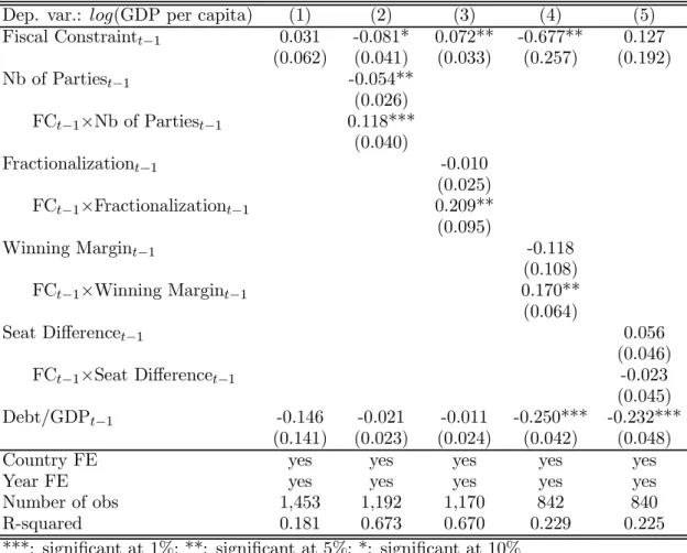
Proposition 2 If a society (β, U, γ,Γ, λ, n) satisfies (17) and n ≥ N0(β, λ), then the
efficient policy g∗ constitutes a symmetric political outcome.
Proof. The left-hand side of (15) is strictly increasing in n, while its right-hand side
does not depend on n. Furthermore, (15) holds with equality for n= N0(β, λ). Thus, if
n≥N0(β, λ), (15) is satisfied. As a consequence,g∗ is a symmetric political outcome.
According to Proposition 2, N0(β, λ)defines the minimum number of parties that can
policy is sustainable in a polity (λ, n), it is also sustainable in a polity (λ, n′), where
n′ > n. In that sense, political competition fosters good economic policy.
Our society can suffer from outcomes that differ from the efficient policy g∗ because
λ >0distorts the objectives of politicians away from those of society at large. Proposition
2 shows that a highncan offset the adverse effects of a positiveλ. However, as Proposition 1 makes clear, such a conclusion holds only if politicians are not too profligate (i.e.,λis not too large). This result becomes particularly relevant when one observes that the differences
gD−g∗ andU(g∗)−U(gD) are weakly increasing functions ofλ. Hence, exactly when the
political distortions can be more severe, competition among the political agents fails to discipline them.
Summing up, in the context studied in this section, where the actions of the political party in office have no bearing on the options available to future governments, there is a
clear sense in which more political competition can foster the implementation of better policies and improve economic performance. As we will see, this is no longer true when current policies can affect the set of actions available to future governments.
4
A society with unrestricted public debt
We now show how the public debt impacts the strategic interaction between politicians. In particular, we will see that it is no longer true that intense political competition fosters the implementation of better economic policies.
As in the previous section, we work with a reduced-form function U(·) that maps
economic policies into household welfare in a competitive equilibrium. In section 3, the period payoff function of a typical household is similar to an indirect utility function that captures the structure of the underlying economy. That function is shaped by the tradeoff between the provision of the public good and its funding. The introduction of public debt
affects that tradeoff. In particular, the vector(bt, gt, bt+1), where bt denotes the
beginning-of-period t value of the public debt, takes on the role that up to nowgt played alone.
In this section we represent the payoff of a typical household by a functionU(bt, gt, bt+1).
That function is shaped by the tradeoff between providing the public good, raising distor-tionary tax revenues19, and managing the public debt. Of course, that tradeoff depends on
19The results of section 3 do not depend on whether or not the government has access to lump-sum
the interest rate, which is a built-in component ofU. In the next subsection we provide an example of a simple dynamic general equilibrium model for which the payoff representation we postulate here either (i) exactly describes or (ii) provides a steady-state approximation of the typical household’s utility. In the latter case, the approximation perfectly matches
the household’s lifetime utility for every equilibrium we study.
4.1
The economic environment
4.1.1 Basic economic structure and competitive equilibrium
We modify the economy of the previous section by allowing the government to issue claims to one unit of the consumption good, redeemable in the next period. Therefore, bt is the
amount of those claims outstanding at the beginning of periodt. This variable is measured
in the same units asgt and its initial valueb0 is exogenous and equal to zero.20 The claims
are traded at a price qt. For notational convenience, we will often denote bt and bt+1 by,
respectively, b and b′.
The government period budget constraint is
gt+bt=τtlt+qtbt+1, (19)
while households’ budget constraint becomes
ct+qtbt+1 ≤(1−τt)lt+bt. (20)
To avoid Ponzi schemes, the public debt must satisfy the constraint |bt+1| ≤ M < ∞,
where M is large enough so that this constraint never binds.
Given {gt, τt, qt}∞t=0, at date t = 0 a household chooses a sequence {ct, lt, bt+1}∞t=0 to
maximize (3) subject to (20) and lt ≤ 1. The necessary and sufficient conditions for this
are (20) taken as equality, (5),
βuc(ct+1, lt+1, gt+1) uc(ct, lt, gt)
=qt, (21)
and
lim
t→∞β
t
uc(ct+1, lt+1, gt+1)bt+1 = 0. (22)
20The assumption b
A competitive equilibrium is composed of sequences {ct, lt}∞t=0, {bt+1}∞t=0 and {qt+1}∞t=0
that satisfy (1) and the optimal behavior of the households for given{gt, τt}∞t=0. A sequence {gt, bt+1}∞t=0 isattainableif there exist sequences{τt}∞t=0,{ct, lt}∞t=0 and{qt+1}∞t=0 such that {ct, lt}∞t=0, {bt+1}∞t=0 and{qt+1}∞t=0 constitute a competitive equilibrium for {gt, τt}∞t=0.
LetH(c, l, g)≡uc(c, l, g)c+ul(c, l, g)l. Using the reasoning of Chari and Kehoe (1999),
we have that the set of attainable sequences is fully characterized by (1) and
∞
t=0
βtH(c
t, lt, gt) = 0. (23)
Additionally, the public debt sequence must satisfy
∞
t=s
βt−sH(c
t, lt, gt) = uc(cs, ls, gs)bs. (24)
4.1.2 The efficient and the dictatorial policies
The efficient allocation{c∗
t, l∗t, gt∗}∞t=0solves the problem of maximizing households’ lifetime
utility (3) subject to (1) and (23). The solution is characterized by those constraints plus the first-order conditions
uc(ct, lt, gt)−θt+ ΘHc(ct, lt, gt) = 0
ul(ct, lt, gt) +θt+ ΘHl(ct, lt, gt) = 0
ug(ct, lt, gt)−θt+ ΘHg(ct, lt, gt) = 0,
(25)
where θt and Θare, respectively, Lagrange multipliers for (1) and (23), while Hc, Hl and
Hg are partial derivatives.
Equations (25), together with (1), establish that {c∗
t, lt∗, gt∗}∞t=0 is a static sequence.
Thus, ∞t=sβt−sH(c∗
t, lt∗, gt∗) =
∞
t=0β
t
H(c∗
t, l∗t, gt∗) = 0 for all s. Hence, (24) implies that
b∗
s = 0 for everys.21
Finally, observe that if b0 = 0, it would be necessary to adduc(c0, l0, g0)b0 to the
right-hand side of (23). As a consequence, the date-0 first-order conditions would be slightly
different; the public debt would be constant and the efficient allocation static only for
t ≥ 1. In summary, if b0 = 0, the efficient allocations and the debt levels would change
fromt = 0tot = 1, and then reach a steady state.
21Naturally, since our environment is not stochastic, there is no role for the tax smoothing property of
As in section 3, assume that the period payoff of a dictator is given byu(ct, lt, gt) +λgt.
The characterization of the dictatorial policy {gD
t , bDt+1}∞t=0 requires finding a sequence {cD
t , ltD, gtD}∞t=0 that maximizes
∞
t=0β
t
[u(ct, lt, gt) + λgt] subject to (1) and (23). The
solution is given by the same equations as the efficient policy except that
ug(ct, lt, gt) +λ−θt+ ΘHg(ct, lt, gt) = 0
replaces the third equation in (25). Thus, bD
t+1 = 0 for all t and the sequence {gtD}∞t=0
is static. Hence, the efficient and dictatorial debt levels are identical. However, as in the economy without debt, government expenditures are inefficiently high under a dictatorship.
4.1.3 Constructing the function U(b, g, b′)
Take an array [b0,{gt, bt+1}∞t=0]. Define U(b0,{gt, bt+1}∞t=0) according to
U(b0,{gt, bt+1}∞t=0)≡ max
{ct,lt}∞t=0
∞
t=0
βtu(ct, lt, gt) (26)
subject to (1), (22), and
ct+β
uc(ct+1, lt+1, gt+1)
uc(ct, lt, gt)
bt+1 =−
ul(ct, lt, gt)
uc(ct, lt, gt)
lt+bt.
This last expression is an implementability constraint for the typical household budget
constraint. It was obtained by combining (20) holding with equality, (5) and (21). By construction,U(b0,{gt, bt+1}∞t=0)is the highest lifetime utility that the household can attain
if the government implements the policy {gt, bt+1}∞t=0.
If there is a function W(b, g, b′) satisfying ∞
t=0β
tW(b
t, gt, bt+1) = U(b0,{gt, bt+1}∞t=0),
then we simply set
U(b, g, b′) =W(b, g, b′). (27)
IfU cannot be decomposed as above, we constructU as follows. Let{g, b′}denote a policy
{gt, bt+1}∞t=0 in which (gt, bt+1) = (g, b′) for every t. Now take a generic vector (b, g, b′). If
each of the arrays [b,{g, b′}] and[b′,{g, b′}] is attainable, then define U(b, g, b′) so that
U(b, g, b′)≡ U(b,{g, b′})−βU(b′,{g, b′}). (28)
debt b and reaches the steady-state (g, b′) after a single period, while U(b′,{g, b′}) is the lifetime payoff in such a steady state. Hence, U(b, g, b′) captures the household utility gain (or loss) associated with that one-period transition. If [b,{g, b′}] or [b′,{g, b′}] is not attainable, then we need to modify our definition. In that case, we setU according to
U(b, g, b′) =U(b,[(˜g(b, b′), b′),{gˆ(b′), b′}])−βU(b′,{ˆg(b′), b′}), (29)
wheregˆ(b′)is the maximum attainable value for g in a steady state with debtb′, ˜g(b, b′)is
the maximum attainable value forg0 when the initial debt is b and the economy will be in
state (ˆg(b′), b′)for every t≥1, and [(˜g(b, b′), b′),{gˆ(b′), b′}] denotes the policy {g
t, bt+1}∞t=0
in which (g0, b1) = (˜g(b, b′), b′) and(gt, bt+1) = (ˆg(b′), b′) for every t ≥1. Observe that we
replaced the values of g specified in the arrays[b,{g, b′}] and[b′,{g, b′}] with the highest
attainable values for that variable. Implicit in our definition is the assumption thatb and
b′ are attainable values for the public debt.
It should be clear that if it is possible to define U as in (27), then U provides an exact
measure of a household’s lifetime utility. If U is defined as in (28) and (29), these two equalities ensure that U perfectly measures the typical household payoff in any steady state or any outcome in which there is a one period transition to a steady state. Since every equilibrium considered in this paper is either static or displays a one period transition
to a steady state, then U is an exact metric of household welfare in those equilibria. We formalize these arguments in the online appendix.
4.1.4 Further economic features
We denote the partial derivatives of U byUb, Ug and Ub′. Similar notation is used for the
second-order derivatives. We assume thatU possesses standard concavity features, so that
Ugg(b, g, b′)<0. Furthermore, we postulate that the partial derivatives satisfy
Ub′(b, g, b′)≥0, Ubg(b, g, b′)<0,Ugb′(b, g, b′)>0, (30)
and Ubg(b, g, b) +Ugb′(b, g, b) < 0. Intuitively, if b and g are held constant, an increase in
b′ reduces the amount of distortionary taxes required to balance the government period
public debt is held constant over time at a level b, then an increase in that level requires, for a fixedg, an increase in the tax burden to service the debt, lowering the marginal utility of g.
The government’s ability to raise tax revenue places bounds on its consumption and
interest expenditures. Let r denote the steady-state interest rate; as usual, r satisfies the equalityβ = (1 +r)−1. Let B >¯ 0denote the maximum value the public debt can reach at
any given date. It has the property that the sumγ+rB¯ is equal to the maximum amount of tax revenue the government can raise in a single period. Observe that if bt+1 = ¯B at
some datet, then(gs, bs+1) = (γ,B¯)for everys ≥t+ 1. That is, if the debt ever reaches its
maximum attainable value, the economy becomes locked in the state (γ,B¯)permanently. The debt may also take negative values. In that case, the typical household becomes a debtor. The household’s ability to repay its debt is bounded by the lifetime income that
it could obtain by working all available time at every date t. Thus, there must be a real number¯b≥0 such that bt≥ −¯b for all t.
The sequence of period budget constraints (19) is the venue through which the date-t
government impacts the set of admissible actions of the future administrators. However, since we want to represent the economic structure in a simple reduced form, we need an alternative way to model the relevant features of (19). As we show next, we achieve that with the help of two very generic functions, fb(b) andfg(b, b′).
Let fb(b) be a strictly increasing and continuously differentiable function. The date-t
government’s choice of bt+1 must satisfy
bt+1∈[fb(bt),B¯]. (31)
Since fb is strictly increasing, a rise in b
t shrinks the set [fb(bt),B¯]. Thus, by increasing
the debt it leaves to its successor, the incumbent at datet−1restricts the choice ofbt+1 of
the next administration. Furthermore, fb( ¯B) = ¯B, because the economy becomes locked
in state (γ,B¯)if the public debt ever reaches the value B¯.
We model the constraints thatbtandbt+1place ongtwith the continuously differentiable
functionfg(b, b′). This function is strictly decreasing inband strictly increasing inb′. The choice ofgt must satisfy
gt∈[γ, fg(bt, bt+1)]. (32)
The role of the upper bound Γ in the previous section is now played by fg(b
t, bt+1). The
set [γ, fg(b
when bt = ¯B, we must havefg( ¯B,B¯) = γ. Suppose now thatbt is equal to some generic
value b for every t. The higher b is, the higher the interest the government must pay, so the tighter its budget constraint is. Hence, the partial derivatives of fg must satisfy
fbg(b, b) +fbg′(b, b)<0.
The party in office at datetcan increasebt+1to enlarge the set from whichgtis selected.
This would restrict the choices of the next administration by tightening constraints (31) and (32). Hence, the date-tincumbent can increase the end-of-period debt bt+1 to achieve
two goals simultaneously: relax the constraints it faces when selectinggt; and tighten the
constraints the government att+1will face when selecting(gt+1, bt+2). In the limiting case
in which bt+1 = ¯B, the date-t incumbent locks the society permanently in state(γ,B¯).
Now let g∗(b, b′) denote the value of g that maximizes U(b, g, b′) under the constraint
γ ≤g ≤fg(b, b′). We assume that ifb <B¯, theng∗(b, b′)< fg(b, b′).22 Furthermore, if the
government keeps its debt constant at some generic level b, the amount of distortionary revenue needed to balance its budget will be a strictly increasing function of b. As a consequence,
b <ˆb⇒U(b, g∗(b, b), b)> U(ˆb, g∗(ˆb,ˆb),ˆb). (33)
In this reduced form representation, the efficient policy is the attainable sequence
{g∗
t, b∗t+1}∞t=0 that maximizes
∞
t=0β
t
U(bt, gt, bt+1). From our analysis of the optimal and
dictatorial policies in 4.1.2, we know that b∗
t+1 = 0. As a consequence, g∗t = g∗(0,0) for
everyt.
4.2
The political environment and the policy game
The political environment is essentially identical to the one of section 3.2; we only sub-stitute U(b, g, b′) for U(g). Therefore, in the present context an economy is an array
(β, U, γ, fg, fb,B¯), apolity is a vector(λ, n), and a society is the combination of an
econ-omy and a polity.
We modify the game of the previous section as little as possible. The players are the same. A history of policies is now an array ht = ((g
0, b1),(g1, b2), ...,(gt, bt+1)). After
observing ht−1, the date-t incumbent selects a policy (g
t, bt+1). The probability that any
given party will be elected is equal to 1/n. A symmetric political equilibrium is defined exactly as before.23 Finally, if {g
t, bt+1}∞t=0 is a symmetric political outcome, then the
22This assumption implies that, givenbandb′, the optimalgis smaller than its attainable upper bound.
Hence, a profligate government has room to overspend without increasing the public debt unlessB= ¯B.
payoff of the date-s incumbent along the equilibrium path is
Ωs({gt, bt+1}∞t=s) =U(bs, gs, bs+1) +λgs+
∞
t=s+1
βt−s U(bt, gt, bt+1) +
λ
ngt . (34)
4.3
The spendthrift equilibrium
We now turn to the characterization of an equilibrium outcome that we will use to support other equilibria by means of trigger strategies. Observe that the task here is not as simple
as in the previous section. For example, even if the date-t incumbent believes that all other parties will implement the dictatorial policy regardless of the history ht−1, it may find it
optimal to issue debt to fund a level of gt above the dictatorial level.
To characterize the equilibria set of our political game, it is convenient to define
G(b, b′, λ)≡arg max
g [U(b, g, b
′) +λg] (35)
subject to24
g ≤fg(b, b′). (36)
Function G(.) defines the level of g that maximizes the incumbent’s period payoff, given (b, b′). The first-order condition associated with this problem is
Ug(b, G(b, b′, λ), b′)≥ −λ. (37)
This condition holds with equality whenever (36) does not bind.
We show in Lemma 2 of the online appendix that G(.) is strictly decreasing in b,
strictly increasing inb′, and weakly increasing inλ. The intuition behind these properties is simple. If g and b′ are held constant, an increase in b requires the government to increase its distortionary revenues. Since the definition of G entails finding an optimal balance between government consumption and distortionary taxation, G decreases as b
rises. Similar reasoning implies thatGincreases inb′. Furthermore, a simple inspection of (35) suggests that Gshould be increasing in λ.25
btand study its corresponding Markov perfect equilibrium. However, it turns out that the efficient policy will not be an equilibrium outcome in such a game. If the date-tincumbent believes that all other parties will implement the policy(gs, bs+1) = (g∗(0,0),0)wheneverbs= 0, then the best action for that player is to set(gs, bs+1)equal to(gD,0). Given our interest in the implementability of efficient policies, we must consider a game that does not have a Markov structure.
24Another constraint isg≥γ, but it never binds.
Suppose that the date-t incumbent believes that all other parties will leave a debt
¯
B regardless of the debt they inherited. If under this assumption the best strategy for the date-t incumbent is to set bt+1 = ¯B, then we have an equilibrium in which the first
incumbent enjoys a relatively high payoff and future governments have no option but to
setgt=γ andbt+1 = ¯B. In particular, for the policy plan
˜
σt(ht−1) = (G(bt,B, λ¯ ),B¯) (38)
to be a symmetric political equilibrium for every ht−1, λ must be sufficiently large. In
this equilibrium, the corresponding outcome is {˜gt,˜bt+1}∞t=0, where g˜t+1 =γ and˜bt+1 = ¯B
for every t, while g˜0 =G(0,B, λ¯ ). That is, the date-0 incumbent sets a value for g0 high
enough to drive the economy to a steady state characterized byγ andB¯. We refer to this
equilibrium and its outcome as the spendthrift equilibrium.26
Since λ measures politicians’ degree of profligacy, at first glance it may seem obvious that the spendthrift policy would be an equilibrium outcome ifλ were large enough.
How-ever, this need not be true. For instance, recall thatbD
t+1 = 0for everyt. Hence, regardless
ofλ, a dictator would not expand the public debt. The reason is that a highλrepresents a penchant for rents today but also in the future, and settingb1 = ¯B would decrease future
rents to their minimum level.
Hence, for the spendthrift policy to be an equilibrium outcome, two conditions must be met:
(C1)politicians are sufficiently profligate;
(C2)the rate at which an incumbent can substitute gt for gt+1 is not too small.
Recall that qt denotes the price of bt+1, in units of gt. By issuing one unit of bt+1 the
government can increase gt by qt units. To balance its date t+ 1 budget, the government
can reduce gt+1 by exactly one unit. Hence, an incumbent can use the public debt to
substitute gt for gt+1 at a rate equal to qt.
The partial derivatives of the date-t incumbent’s payoff with respect to gt andgt+1 are
equal to, respectively, Ug(bt, gt, bt+1) +λ andβ[Ug(bt+1, gt+1, bt+2) +λ/n]. Therefore,
− dgt
dgt+1
=βUg(bt+1, gt+1, bt+2) +λ/n Ug(bt, gt, bt+1) +λ
,
(b, b′, λ). As a result, the partial derivativesG
b,Gb′, andGλmay be undefined at those points.
26The spendthrift equilibrium shares some characteristics with the financial autarky equilibrium of
where−dgt/dgt+1is a standard intertemporal marginal rate of substitution. Thus, the date-t incumbent has an incentive to increase gt and to reducegt+1 by issuing debt whenever:
qt> β
Ug(bt+1, gt+1, bt+2) +λ/n
Ug(bt, gt, bt+1) +λ
. (39)
Inequality (39) reveals how the combination of political competition with conditions (C1) and (C2) brings forth the spendthrift equilibrium. Make λ → ∞. Since Ug is
bounded, the right-hand side of (39) converges toβ/n. Hence, forλ sufficiently large, (39) holds whenever
qt> β/n. (40)
It is well known from basic macroeconomics that if an economy is in a deterministic steady state, qt = β. Thus, if λ is large and qt is not considerably smaller than its steady-state
value, the date-t incumbent will have an incentive to issue debt and increasegt.
We formally establish in the online appendix that if conditions (C1) and (C2) are satisfied, then the spendthrift policy is an equilibrium outcome. For condition (C1), we require that
λ >λ˜, (41)
where λ˜ is a real number whose existence is established in that appendix.27 In turn,
condition (C2) entails placing a lower bound on qt. Since that variable is not an explicit
component of our political game, we must disentangle it from the whole structure of the
game.
To do so, take a policy {gt, bt+1}∞t=s with the property that gt = G(bt, bt+1, λ). For
simplicity, assume that the partial derivativesGb andGb′ are defined at every point(b, b′, λ).
Let t be any date and δ be a small positive number. If bt+1 increases by δ, gt will grow
by approximatelyδGb′(bt, bt+1, λ), whilegt+1 will fall by approximately−δGb(bt+1, bt+2, λ).
Hence, a policymaker can substitutegt for gt+1 at the rate
− δGb′(bt, bt+1, λ)
δGb(bt+1, bt+2, λ)
=− Gb′(bt, bt+1, λ)
Gb(bt+1, bt+2, λ)
.
However, the rate at which a policymaker can substitute gt for gt+1 is also equal to qt.
27When λ ≤ λ˜, one can show that if U(.) satisfies some regularity conditions, then there exists an