FUNDAÇÃO GETÚLIO VARGAS
ESCOLA DE ADMINISTRAÇÃO DE EMPRESAS DE SÃO PAULO MPA – MESTRADO PROFISSIONAL EM ADMINISTRAÇÃO
SURAYA MARCONDES CABRAL VILLAR
THE DETERMINANTS OF FOREIGN DIRECT INVESTMENT DISTRIBUTION
AMONG THE BRAZILIAN STATES
SURAYA MARCONDES CABRAL VILLAR
THE DETERMINANTS OF FOREIGN DIRECT INVESTMENT DISTRIBUTION
AMONG THE BRAZILIAN STATES
Dissertação apresentada à Escola de Administração de Empresas de São Paulo, da Fundação Getúlio Vargas, como requisito para obtenção do título de Mestre em Administração Empresas.
Linha de Pesquisa: Finanças
Orientador: Prof. Dr. Hsia Hua Sheng
FICHA CATALOGRÁFICA
Villar, Suraya Marcondes Cabral.
The determinants of foreign direct investment distribution among the Brazilian states / Suraya Marcondes Cabral Villar – 2014. 57f.
Orientador: Hsia Hua Sheng.
Dissertação (MPA) - Escola de Administração de Empresas de São Paulo.
1. Investimento Estrangeiro - Brasil. 2. Análise de painel. 3. Incentivos fiscais. I. Hua Sheng, Hsia. II. Dissertação (MPA) - Escola de Administração de Empresas de São Paulo. III. Título.
SURAYA MARCONDES CABRAL VILLAR
THE DETERMINANTS OF FOREIGN DIRECT INVESTMENT DISTRIBUTION
AMONG THE BRAZILIAN STATES
Dissertação apresentada à Escola de Administração de Empresas de São Paulo, da Fundação Getúlio Vargas, como requisito para obtenção do título de Mestre em Administração Empresas.
Linha de Pesquisa: Finanças
Orientador: Prof. Dr. Hsia Hua Sheng
Aprovada em: 08.12.2014
Banca Examinadora:
_____________________________
Prof. Hsia Hua Sheng FGV-EESP
_____________________________
Profa. Mayra Ivanoff Lora FGV-EESP
ACKNOWLEDGEMENTS
I would like to express my sincere gratitude to my advisor, Professor Hsia Hua Sheng, for his patient and generous encouragement. I also would like to thank my co-advisor, Professor Mayra Ivanoff Lora for her insights and questioning. My gratitude to Professor Adriana Bruscato Bortoluzzo for her generosity and availability.
I am specially thankful to all of the professors of the EAESP – FGV MPA course for their assistance and advice. I am also thankful to all my colegues, for learning and for the friendly atmosphere during the course.
“We can easily forgive a child who is afraid of the dark; the real tragedy of life is when men are afraid of the light.”
ABSTRACT
Villar, S. M. C. The determinants of foreign direct investment distribution among the
Brazilian states.2014. 57f. Tese (Mestrado) - Escola de Administração de Empresas de São
Paulo, Fundação Getúlio Vargas, São Paulo, 2014.
FDI has played an important role in Brazil’s push towards a market oriented economy. From 1995 to 2012, Brazil has received $ 511.5 billion dollars in FDI. In 2012 Brazil was the second largest developing country recipient of FDI and the fourth worldwide (UNCTAD).Due to geographical concentration, Brazilian states which are considerably less developed and poorer, and as a result, in greater need of capital investment, have not played host to FDI in a significant way. In 2010, states with the largest stocks of FDI were São Paulo with 42.3 percent of the total ($ 99.9 billion dollars), Rio de Janeiro with 13,3 percent ($ 31.4 billion dollars) and Minas Gerais with 10,6 percent of the total ($ 25.1 billion dollars). As can be observed, only three of the twenty-seven Brazilian states received around 66 percent of the total FDI intended to Brazil.Given such differentiation in the distribution of FDI among Brazilian states, this study seeks to explain if tax benefit is also a determintant of FDI inflow, besides the other variables already considered as determinant. Given the limitation of data, we performed two econometric analysis with panel data: 1. using six key variables: size of the consumer market, quality of workforce, transportation infrastructure, cost of labor, tax burden and tax benefit (by macro regions), in the years 1995, 2000, 2005 and 2010; 2. using five key variables: the same as the first model, excluding the cost of labor (for lack of data) and using the tax benefit data by state, in the years 2010, 2011 and 2012.
RESUMO
Villar, S. M. C. The determinants of foreign direct investment distribution among the
Brazilian states.2014. 57f. Tese (Mestrado) - Escola de Administração de Empresas de São
Paulo, Fundação Getúlio Vargas, São Paulo, 2014.
O Investimento Estrangeiro Direto (IED) tem desempenhado um papel importante no esforço do Brasil para tornar-se uma economia orientada para o mercado. De 1995 a 2012 o Brasil recebeu $ 511.5 bilhões de dólares em IED. Em 2012, o Brasil foi o segundo país em desenvolvimento que mais recebeu IED e o quarto no mundo (UNCTAD).Devido à concentração geográfica, os estados brasileiros que são consideravelmente menos desenvolvidos e mais pobres, são aqueles que mais precisam de investimentos e que no entanto, não têm sido receptores relevantes de IED. Em 2010, os estados com os maiores estoques de IED foram São Paulo, com 42,3 por cento do total ($ 99,9 bilhões de dólares), Rio de Janeiro com 13,3 por cento ($ 31,4 bilhões de dólares) e Minas Gerais com 10,6 por cento do total ($ 25,1 bilhões de dólares). Como pode ser observado, apenas três dos vinte e sete estados brasileiros receberam cerca de 66 por cento do total de IED destinado ao Brasil.Dada tal diferenciação na distribuição de IED entre os estados brasileiros, o presente estudo busca explicar se o benefício tributário também é determinante para o fluxo de IED, além das demais variáveis já consideradas como determinantes em outros estudos. Dada a limitação de dados, realizamos duas análises econométricas com dados em painel: 1. Usando seis variáveis chaves: tamanho do mercado consumidor, a qualidade da mão de obra, infraestrutura, custo da mão de obra, carga tributária e benefício tributário (por macro regiões), nos anos de 1995, 2000, 2005 and 2010; 2. Usando cinco variáveis: as mesmas do primeiro modelo, excluindo o custo da mão de obra (por falta de dados) e utilizando os dados de benefício tributário por estado, nos anos de 2010, 2011 e 2012.
Palavras-chaves: Investimento estrangeiro direto. Estados brasileiros. Dados em Painel.
LIST OF FIGURES
Figure 1 - Top 20 host economies, 2012 (billions of dollars) ……… 19
Figure 2 - FDI distribution among Brazilian states – 2012 ……….. 20
LIST OF TABLES
Table 1 - FDI inflow by investor country ……… 18
Table 2 - Gross tax burden ……… 21
Table 3 - Breakdown tax collection ……… 22
Table 4 - Descriptive statistics of the variables (model A) ……… 35
Table 5 - Pearson correlation (model A) ……… 48
Table 6 - VIF (model A) ……… 49
Table 7 - Descriptive statistics of the variables (model B) .………… 38
Table 8 - Pearson correlation (model B) ……… 49
Table 9 - VIF (model B) ………... 50
Table 10 - OLS – Ordinary least square (Model A) ……… 50
Table 11 - OLS – Ordinary least square (Model B) ……… 51
Table 12 - Expected effect ……… 41
Table 13 - Model A ……….………… 52
INDEX
1 INTRODUCTION……… 13
2 LITERATURE REVIEW………... 16
2.1 Foreign direct investment in Brazil ………... 16
2.2 Tax concept ………. 21
2.3 Fiscal war ………. 26
3 RESEARCH METHODOLOGY ……… 31
3.1 Tax incentive variable ……….. 31
3.2 Description of variables ………... 33
3.3 Model ………... 39
4 RESULTS ………..… 42
5 CONCLUSION ……….… 46
LIMITATIONS ……… 47
APPENDIX ……….. 48
1 INTRODUCTION
During last decades, foreign direct investments (FDI) played an important role in the globalization process and have been crucial in the development of local businesses and economies in the host countries. According to the International Monetary Fund (IMF), FDI is defined as an investment involving a long-term relationship and reflecting a lasting interest in and control by a resident entity in one economy (foreign direct investor or parent enterprise) of an enterprise resident in a different economy (FDI enterprise or affiliate enterprise or foreign affiliate). Such investment involves both the initial transaction between the two entities and all subsequent transactions between them and among foreign affiliates.
In Brazil, the FDI inflow started to be more significant after the creation of Plano Real, which aimed important economic reforms. Thus, due to greater economic stability, FDI inflow more than doubled from 1994 to 1995 reaching $ 4.4 billion dollars (UNCTAD). In the following years, until 2000, the country saw the FDI inflow eightfold, reaching $ 32.8 billion, mainly driven by privatization that occurred in different sectors. Despite the decline of this flow in the following years, from 2007, the investments resumed their previous levels and according to the Brazilian Central Bank (BC), from 2008 to 2012, while the balance of current transactions showed a $ 206.5 billion dollars accumulated deficit, FDI exhibited a $ 251.4 billion dollars surplus, helping to alleviate the need to finance the Brazilian balance of payments. Therefore, it is clear the importance of this type of investment in the Brazilian economy.
To reinforce this importance, Carminati and Fernandes (2012) analyzed the relation between the GDP and the FDI for the Brazilian economy in the period of 1986 and 2009. This study used the Structural VAR model and also anylized others variables as exchange reate, electric energy consumption, tax for imported product, inflation and economic stability. The conclusion showed that FDI has a positive effect on the GDP.
in shaping economic activity. The result suggested that there is a positive relationship between the ration of FDI stock / GDP in the states and growth in GDP per capita.
According to De Angelo, Eunni and Fouto (2010) who studied the determinants of FDI in emerging markets with a focus on Brazil during the period of 2000 until 2007, concluded that the evolution of the consumer market and strength of consumer sales are more important in explaining capital movements into Brazil than other factors as interest rates, exchange rates and country risk.
Baer and Rangel (2001) also gave their contribution by analyzing the FDI inflow to Brazil from 1929 until 1998. The study is divided in three mainly categories: 1. the era of the export economy, which comprises the period of 1929 until the 40s; 2. the era of import substitution, from the 50s until the 80s, when multinationals were attracted to build import substitution facilities in many sectors as they had the capital and the technology that domestic private and public firms did not have. Finally, 3. the era of neo-liberalisn in the 90s, where we had the opening of the economy mainly driven by the privatizations that occurred in this period.
Another analysis related to Brazil and FDI came from Aguiar, Conraria, Gulamhussen and Magalhães (2012) who related the FDI with the home country political risk. Their findings revealed that higher levels of home-country political risk lead to lower levels of FDI into Brazil and also that the negative relationship between risk and FDI into Brazil is associated with poor quality of policies we have.
inquiry is whether the tax benefit, as well as the tax burden is also significant for the determination of FDI in a particularly state. To improve previous analyses we segregated the tax issue in two variables: one specific to measure the tax burden, which is ICMS/GDP and another to measure tax incentives, represented by tax expenditure/GDP. Thus, we got a clear way to assess the impact of each of this variables on the FDI inflow to the states.
As noticed, we do not have a vast literature about FDI in Brazil and little has been reported reported on the destination of FDI among the Brazilian states. Also, until the conclusion of this study we found no literature that relates FDI with tax incetives at the level of Brazilian states. Therefore, we believe that this is the greatest contribution of this paper.
2 LITERATURE REVIEW
2.1 Foreign direct investment in Brazil
The period from the end of World War II until the late 1970s foreign multinational companies started to integrate to some of the Brazilian public and private firms. (Hiratuka and Sarti, 2010). However, with the economic crisis of the 1980s, the entries of FDI in Brazil were strongly reduced compared to 1970 from USD 2.3 billion in the period 1971-81 to only USD 357 million between 1982 and 1991. Agudelo and Tebaldi (2004) explain that this reduction was due to ineffective and recessive economic adjustments that caused a reduction on profit rates in the productive sectors, discouraging new investment and increasing profit remittances to countries of origin of the transnational companies, who maintained their ability to accumulate capital . Thus, the transnational and multinational companies already operating in Brazil, were in search of reducing its indebtedness and preserving profitability, which somehow ended up hindering the process of modernization.
One of the major barriers to FDI in Brazil was the high rates of inflation. In 1994 Brazil had a major evolution in its economy in the deployment of the Real Plan. Part of this plan was the creation of a new currency which brought a greater stability of the inflation, the annual rate of inflation was 5.150 percent and was brought down to about 10 percent at the end of the program (De Angelo, Eunni and Fouto, 2010). The new plan also brought the possibility of the renegotiation of the country foreign debt. Combined with this factors, the reduction of economic restrictions also boosted the trade openness of the country.
In order to assess the presence of FDI in the country, the Central Bank of Brazil (BC) held its first Census of Foreign Capital in 1995. The census was conducted through a questionnaire answered by the companies that had its operations registered in the Department of Foreign Capitals at BC. The result showed a stock of FDI at December 31st, 1995 amounting to USD 41.7 billion, which about a quarter came from the United States. The main target of this type of investment in Brazil was the Industry sector, which had received 67 percent of the total inflow of FDI. Three industries accounted for almost half of investment, in order of relevance: the chemicals sector, automotive sector and finally the metallurgy.
due to the deregulation of the financial sector. Nonetheless, it was after the implementation of Real Plan that the flow of the privatizations were intensified. According to Lacerda (2004), the privatizations carried out in federal and state levels generated a cumulative total revenue of USD 87.2 billion in the period of 1991 to 2002. Of this total, the share of foreign capital reached 48.3 percent, representing an annual average of about 24.76 percent of the total collected in the period of 1996 to 2000. This was the most significant period regarding the inflow of FDI related to privatization, because after 2001 there has been a drop, reaching 1.5 percent in 2002.
In this period, we also had in Brazil a number of large private companies of national capital being acquired by foreign owned companies. Some examples are: Metal Leve, Lacta, Renner Group, Cofap, Agroceres and some banks as Nacional-Excel, Bamerindus and Real (Ribeiro and Sambatti, 2002). According to Carneiro (2002), M&A happens when a company can quickly win market share by absorbing competitors or even have access to new markets by acquiring brands with local tradition. Also, in accordance with the Research Institute for Industrial Development (IED), Brazil showed a participation in M&As above the average for developing countries, almost reaching developed contries numbers in this period.
Until 1998, Brazil kept the regime of bands for the exchange rate in order to maintain the inflation under control, which favored the increase of FDI inflow in the Brazilian economy in general and in particular on privatization and M&As (Ribeiro and Sambatti, 2002). However, from 1999, the exchange rate regime became floating, which was one of the reasons that had contributed to a decline in FDI inflows directed to privatization. (Lacerda, 2004).
In the second Census of Foreign Capital, for the year 2000, the Service sector accounted for almost 64 percent of the total FDI inflow, followed by the Industry with 33.71 percent. This results were still regarded to the previtatizations in the infrastructure and telecommunication sectors (Lacerda and Oliveira, 2009). The stock of FDI at December 31st, 2000 more than double compared with 1995, reaching USD 103 billion. The main contributor was still the United States, with nearly 24 percent participation on the inflows of FDI to Brazil (BC).
macroeconomic conditions as inflation, public accounts and external accounts, besides the rate of growth of domestic demand, Brazil`s GDP grew at a rate exceeding 3 percent, with domestic demand accounting for 85 percent of GDP (BC).
Among Latin American countries, Brazil ranked first in 2008 in FDI inflows in the region, followed by Mexico and Chile. The high oil prices and commodity stimulated the growth of FDI in Latin America and Caribbean. In the region, inflows rose 36 percent reaching USD 126 billion. Also, considering all developing countries, Brazil has positioned itself in fourth in FDI inflows, with USD 34.6 billion in 2007, surpassed only by China (USD 83.5 billion), Hong Kong (USD 59.9 billion) and Russia (USD 52.5 billion) (UNCTAD).
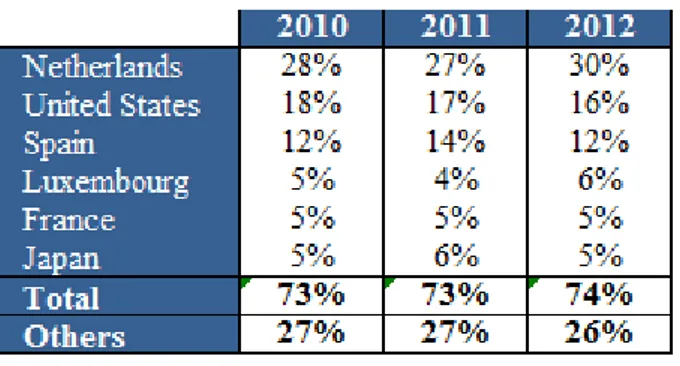
Table 1 shows that in the period of this study, 2010 - 2012, foreign capital flows mainly from Netherlands and United States with around 50 percent of the total foreign capital and then they were followed by Spain, Luxembourg, France and Japan. All being the main countries responsible for 74 percent of FDI inflow in Brazil (BC).
Table 1 - FDI inflow by investor country Source: Adapted from Central Bank of Brazil
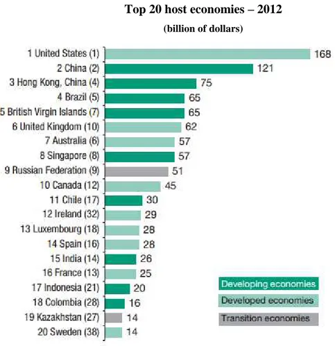
Top 20 host economies – 2012 (billion of dollars)
Figure 1 - Top 20 host economies, 2012 (billions of dollars) Source: UNCTAD, World Investment Report 2013
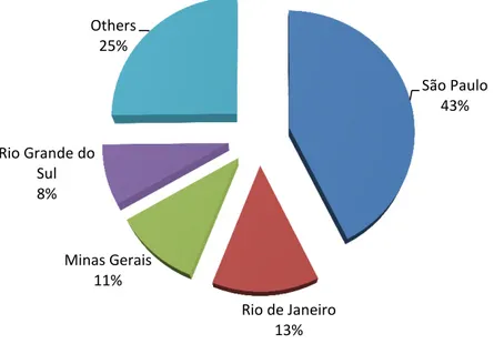
FDI distribution among Brazilian states - 2012
Graphic 1 - FDI distribution among Brazilian states - 2012 Source: Adapted from Central Bank of Brazil
Hymer (1960) explained that multionational companies were the result of imperfect market and monopoly advantages. Hence, FDI tends to flow into differentiated markets where the multinationals will have a competitive advantage. However, still according to Hymer (1960) it is crucial that the company that inteds to invest overseas already present advantages related to economies of scale, special skills, low-cost production or differentiated products.
According to Dunning (1997), multinationals corporations will invest in a foreign country if it offers certain location advantanges in terms of resources and facilities that will aggregate value for the multinational. Brazil is the largest Latin America country and it provides access to a wide diversity of markets not only in Latin America, but also in Central and North America. On the economic side, Brazil presented a GDP of approximately USD 2.2 trillions in 2012 (BC) which is a convicing record of development as an emerging economy and a financial centre for the region. Moreover, Brazil’s growing domestic market comprises almost 200 million people (IBGE), which is equivalent the population of France, Italy and Germany combined. Thus, this show the great potential of the internal market that represents growth for many companies.
After reviewing the historical flow of FDI in Brazil, we will treat the next sessions on tax benefits, since the main interest of this study is to assess whether ot not those incentives
São Paulo 43%
Rio de Janeiro 13% Minas Gerais
11% Rio Grande do
Sul 8%
impact the flow of FDI among the Brazilian states. Therefore in the next session we will address key concepts of taxes and then evaluate the reaserch methodology.
2.2 Tax concepts in Brazil
Before discussing the tax benefits in Brazil, it is important to clarify some concepts in this area. For this, we rely on Almeida (2000), Nascimento (2008), Paranaiba and Marques (2013).
Analysing the different forms of existing collection in Brazil, we have: taxes, fees and contributions for improvement. The tax triggering event is an independent situation of any particular state activity that is related to the taxpayer. The fee refers to a specific public service that is provided to the taxpayer or that is at his disposal. Finally, the contribution of improvement refers to the public works that generate real estate valuation. Thus, the value of this contribution shall be limited to the total amount of expenditure on such works that are divided with every property that will benefit from this public work. These are the items that comprise the forms of tax collection.
As it can be seen in the table below, the tax revenue in Brazil represented, on average, 34.70 percent of GDP in the period 2000-2010.
Table 2 - Gross Tax Burden (BRL millions) Source: Adapted from Treasury Department
The tax revenue of the Union consists of three categories of taxes: a) taxes of Federal Government, which mainly include the Income tax, tax on imported products (Imposto Sobre Produtos Industrializados - IPI), contribution to the Social Security and contribution to the financing of Social Security (Cotribuição para o Financiamento da Seguridade Social – COFINS); b) taxes from the State Government – in which the Tax on Circulation of Goods and Supply of Services (Imposto sobre a Circulação de Mercadorias e sobre Prestações de Serviços de Transporte Interestadual, Intermunicipal e de Comunicação - ICMS), has almost all participation; c) taxes of Municipal Government, mainly composed by tax on any service
2000 2005 2010
Gross Domestic Product 1.089,68 1.937,70 3.674,96 Gross Tax Collection 361,47 724,11 1.233,49
of any nature (Imposto Sobre Serviço de Qualquer Natureza - ISS) and the property tax (Imposto Predial e Territorial Urbano - IPTU).
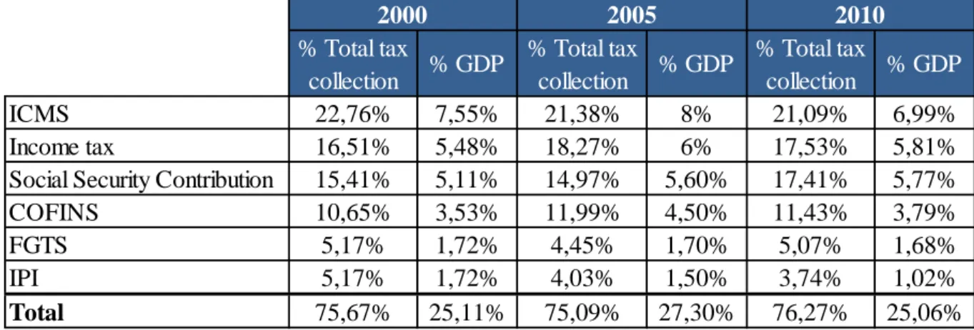
In table 3, we can see that the main source of collection of the Union comes from ICMS, which is a tax of the State Government level. We can also verify that the six main taxes correspond, on average, about 75.68 percent of total collection and 25.82 percent of the country GDP.
Table 3 - Breakdown tax collection
Source: Adapted fromTreasury Department
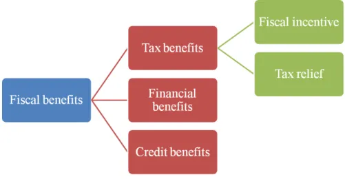
On the other side, we also have the concepts related to tax benefits and collection losses. The Federal Constitution of 1988, article 165 § 6 establish three types of benefits: financial, tax and credit. Together they constitute the set of fiscal benefits.
It is considered tax benefit any form of exemption, remission or reduction of assessment basis or of tax rate that should be collected. These benefits are special disposals to the general tax rule given to a select group of taxpayers, economic sectors or geographical regions to achieve goals of economic, social or administrative order, thus, encouraging the development of a particular region.
Still within the group of tax benefit, we have two subgroups: fiscal incentives and tax reliefs. For a fiscal incentive to be considered a tax benefit, it is necessary that this benefit induces the behavior of taxpayers, in other words, that stimulates these taxpayers to act in a certain way. An example of fiscal incentive is the absence of income tax on earnings from savings accounts. In this case, the incentive was given to attract individual taxpayers to carry out this type of investment, encouraging savings rather than consumption. The tax relief, as
% Total tax
collection % GDP
% Total tax
collection % GDP
% Total tax
collection % GDP
ICMS 22,76% 7,55% 21,38% 8% 21,09% 6,99%
Income tax 16,51% 5,48% 18,27% 6% 17,53% 5,81%
Social Security Contribution 15,41% 5,11% 14,97% 5,60% 17,41% 5,77%
COFINS 10,65% 3,53% 11,99% 4,50% 11,43% 3,79%
FGTS 5,17% 1,72% 4,45% 1,70% 5,07% 1,68%
IPI 5,17% 1,72% 4,03% 1,50% 3,74% 1,02%
Total 75,67% 25,11% 75,09% 27,30% 76,27% 25,06%
the name implies, is used to relieve situations of involuntarily taxpayers difficulties. An example, in this case, is the tax exemption given on earnings from retirement and pension plans that are paid by the public social security for people over 65 years. The purpose here is to alleviate the contribution, so that the retired can enjoy a more favored social condition.
Figure 3 illustrates the types of fiscal benefits:
Figure 3 - Fiscal benefits
Source: Figure adapted from Almeida, 2000
The first experience of quantification of tax benefits occurred in Germany in 1959, and since 1967 they created a legal requirement to insert the given budget. Other countries have followed this practice, as the United States, starting in 1968, Spain, the UK, Austria and Canada, from the 1970s (Bordin 2003). Brazil did its first publication in 1989, the report is provided by the IRS, and continued to do so on a yearly basis. From 1991 until 2003 the report was named Statement of Tax Benefit (Demonstrativo dos Benefícios Tributários – DBT), then from 2003 until 2008 was Statement of Governement Spending of Indirect Tax – Tax Expenditure (Demonstrativo dos Gastos Governamentais Indiretos de Natureza Tributária – Gastos Tributários) and from 2009 until 2013 it was again renamed for Statement of Tax Expenditure (Demonstrativo dos Gastos Tributários – DGT).
[…] The second element consists of the special preferences found in every
income tax. These provisions, often called tax incentives or tax subsidies, are departures from the normal tax structure and are designed to favor a particular industry, activity, or class or persons. They take many forms, such as permanent exclusions from income, deductions, deferrals of tax liabilities, credits against tax, or special rates. Whatever their form, these departures from the normative tax structure represent government spending for favored activities or groups, effected through the tax system rather than through direct grants, loans, or other forms of government assistance.
International organizations like the OECD, the World Bank and the IMF also quickly moved on to study tax expenditures. The OECD has repeatedly addressed the topic and his latest publication on the subject (OECD, 2010) provides a comprehensive study of tax expenditures in ten member countries. Already the IMF has adopted different authority providing general guidelines for the application of tax expenditures with the publication of several editions of the Manual on Fiscal Transparency, the latest in 2008. In a complementary way, the World Bank's approach to present the experiences of the countries most developed to assist developing countries in the structure of the legislation and estimation of tax expenditures.
In Brazil, the budget organization begins with the Multi-Year Plan (Plano Plurianual – PPA) where the macro guidelines for the following four years are specified. For this Plan to work as planned, we have the Budget Guidelines Law (Lei de Diretrizes Orçamentárias – LDO) that brings a series of rules of how to design, organize and implement the budget. In addition, is in the LDO where we have the definitions of which investments will be prioritized, including the investment policy of the development agencies. For all this planning to be put into practice, considering a short therm view, we have the Annual Budget Law (Lei Orçamentária Annual – LOA). Is in the LOA where we have the forecast of all the revenues and expenses for a specific year. On the expenses side, is where we have the tax expenditure disclosure, with all the benefits that are expected to be provided. Each Brazilian state has its own PPA, as well as their respective LDO and LOA. However, all these guidelines follow the main guideline of the Federal Government.
preservation of public property, limit public spending, management of fiscal risks, broad access to information on public accounts.
It is up to the Federal Government promote an optimal allocation of scarce resources, alleviate the unequal distribution of wealth, minimizing regional imbalances in income and create conditions for monetary and fiscal stabilization. Since the Second World War, many countries have used fiscal instruments to accelerate the pace of economic development and in Brazil this has been no different. The Federal Government has several incentive programs, with the main being:
- Free Zone of Manaus (Zona Franca de Manaus): was established in 1967 to boost economic development in Amazonia state. This project is manager by the Superintendency of the Manaus Free Zone (Superintedência da Zona Franca de Manaus – SUFRAMA) and has around 720 industries that comprises three economic sectors: commercial, industrial and agricultural. Since its creation, the companies that are installed there count on huge tax incentives that was given for a period of 30 years and has been renewed over the years. In this case, we have a period of 47 years with concession, without any hint of termination or revision of the coditions.
- SUDENE: was created in 2002 under the name ADENE – National agency for development of the Northeast (Agência Nacional de Desenvolvimento do Nordeste). Than it was renamed to Sudene – Superintendency for development of Northeast (Superintendência do Desevolvimento do Nordeste). Its mission is to promote inclusion and sustainability of their area of operation and the competitive integration of regional production base in the national and international economy.
- REPORTO: this program is a tax incentive for odernizatio and expansion of the port structure and was established on December 1st, 2004. This tax regime suspend the collection of: tax on industrialized products (IPI), the contribution to the financing of Social Security (COFINS) and when applicable, the import tax on the sales of machinery, equipment ad other goods in the port terminals.
other hand, the most common criticism is that exemptions are a form of waste government resources, as the incentive may be given to the taxpayer that would invest regardless of the existence of the benefit. In addition, the tax expenditure could distort the choice of market alternatives, removing the neutrality that should exist in the allocation of private resources process. Thus, the benefit should interfere as little as possible in decisions about investment and business organization.
Although the Complementary Law is relatively recent, the next step for the improvement of the Fiscal Responsibility Law would be the evaluation of the results of the tax expenditure. This would require setting paramenters of the population welfare to control these assessments. Therefore, while Brasil still does not have these evaluation mechanisms, we incurred in what we call fiscal war, the subject of our next session. We will see that the tax benefits are often granted without the proper analysis of returns of that benefit. Most importantly, the states end up competing investments and grating benefits only seeking their own interests.
2.2 Fiscal War
Brazil lived for 21 years a regime of dictatorship, which began in 1964 with a military coup that overthrew the government of President João Goulart. Only in 1985, this regime ended, and we had the New Republic. This was a period of great changes for the country, which had its Constitution promulgated in 1988. As explained by Dulci (2002), one of the major changes brought by the new Constitution was a greater power to each of the 26 units of the Brazilian Federation plus the Federal District, in several aspects, including the tax issue. One of the most important points was that each state began to have autonomy to set the aliquot of ICMS, the main source of tax collection, as we saw earlier.
There has been a record of fiscal disputes in Brazil since the 20s, though it was in the 90s, with the opening of the economy, that this dispute has been intensified (Nascimento, 2008). Brazilian states saw on entry of foreign capital in the country an opportunity to attract these investments to generate jobs, increase income, promote the economy to increase GDP and consequently increase tax collection.
According to Nascimento (2009), the so-called fiscal war occurs both between the Federation Units and the Union, and among the Federation Units. In the first case, since the Constitution of 1988 was promulgated, there has been an increase in the collection of taxes by the states, as a result of tax changes. Therefore, the Union had its tax collection reduced, and the way found to expand this collection was to create or increase the aliquot of social contributions that are not subject to have a share transfer to the states. In the second case, the competition between the Federation Units happens in two ways: among the states, by charging a different aliquot of ICMS for the same services, and among municipalities, through the differences of the charge of ISS and IPTU. Thus, each region ends up creating "artificial" advantages for enterprises to choose regions that, perhaps, by the logic of the market, would not be chosen to be installed.
In this fiscal dispute, it is clear the advantage of powerful multinationals versus local companies. While, in the first case, the multinationals are highly benefited with various tax benefits, the others end being charged for full payment of due taxes. So the government starts to deal with a scenario of default and tax evasion by companies that do not agree with the distribution of tax collection. As a consequence, we have the “informal economy”, representing an important part of the Brazilian economy (Prado, 1999).
There are several examples of fiscal war in Brazil and different industries that are affected. Lagemann (2014) made a specific study on the fiscal war in Brazilian ports. The supplementary Law No. 87 (LC 87/96) of September 13, 1996, which defines the ICMS, in Article 12, defines that the triggering event of payment of the tax should happen in customs clearance, and the chargement of the tax should be made at the place in which the goods are delivered. Thus, the tax responsibility, in this case, is of the place that receives the delivery, and not of the place where, in fact, the product or service will be consumed and / or used. As the delivery and consumption might not occur at the same location, a state ends up with the tax revenues that should belong to another state. In addition, the consumer will use the public services of the state he is, but, on the other hand, there is no payment of taxes due to this state. Additionally, it is evident that the port states are encouraged to stimulate the installation of companies in which the delivery occurs. So they can appropriate of the tax revenues that should belong to the states where end consumers are.
In the automotive industry, one of the most emblematic cases was that of Ford Company. In 1999, the new government in Rio Grande do Sul decided to review the benefits given to the company by considering that it was too costly to the state. Ford tried to convince the government to keep the agreement, and, if that did not happen, the company would install its new plant in another state. Observing this impasse, the government of Bahia quickly asked the Federal Government to reopen the program of incentives for the automotive industry in the Northeast, which had ended in the previous year. Due to the federal political alliances with the state of Bahia, the Federal Government gave in to this request, which caused a political discomfort, not only with the state of Rio Grande do Sul, but with other states that considered inappropriate the intervention of the Federal Government on this issue. Besides the renunciation of federal taxes, Ford had a loan from BNDES, and other benefits offered by the Bahian government (Incentivo à Montadora, 1999).
When evaluating the fiscal war in meat and leather industry, the state of Minas Gerais was even more harmed. Their competitors in this sector, the states of Ceará, São Paulo, Mato Grosso do Sul, Bahia and Espírito Santo, completely eliminated the ICMS tax aliquot. As a result, in four years, in the period 96-00, Minas lost 17 refrigerators to the states of Goiás and São Paulo. (Frigoríficos Insatisfeitos, 2000).
In accordance with Diniz (2000), fiscal war is harmful to the public treasury, endanger future collections besides causing changes in prices. The war ends up benefiting more developed states, which have greater financial and political conditions to afford larger fiscal renunciation. These factors exacerbate the inequalities among the regions, as we talked earlier in this session.
According to Ozaki and Biderman (2004), this dispute also reached the municipal spheres. As it was mentioned earlier, the tax used in municipalities dispute is the ISS. The Complementary Law 116/03 updated and regulated the ISS legislation, expanding the list of taxable services for 193 items. The triggering event for the collection of this tax is where "the service will be provided”. This term is considered to be subject to different interpretations because one might consider that the service will be provided in the central office or in the parent company, that is, in the specific address where the company is located. However, it may be that the service is performed elsewhere.
The fiscal war on ISS can be considered more serious than the one with ICMS. Even with the enactment of Constitutional Amendment 37 of 2002, which set the floor of the aliquot at 2%, we have municipalities that charges lower rates, hurting the Constitution with illegal act. This is not the only problem. We also have a fraud scenario: companies that “fictitiously” install themselves in a municipality, keeping only an address, without having any activity in that place just to take advantage of the tax benefit in that municipality (Martins and Cintra, 2006).
Almeida (2000) brought an important contribution by analyzing all the problems related to fiscal renunciation:
Another important goal is the development of strategic economic sectors that favors certain groups of taxpayers, among other relevant public goals.
Because of these disputes between the states that we just described, we believe that the tax benefit has influence in the decision of which state will receive the FDI. However, still according to Almeida (2000), the difference between Brazil and developed countries is that they have instruments to control the results achieved with the given benefits. Thus, these countries can know whether the adopted fiscal policy is being effective.
3 RESEARCH METHODOLOGY
3.1 Tax incentive variable
As previously mentioned, this study aims to make an unprecedent assessment of the impact of the tax incentive in FDI of Brazilian states. To achieve this result, we performed an econometric panel regression using two models: A – for the years 1995, 2000, 2005 and 2010, with the tax expenditure by macro regions; B – the period of 2010, 2011 and 2012, with the tax expenditure variable by state.
The tax expenditure is a variable used in many studies to analyze how this fiscal policy impacts the FDI inflows in a certain country or region. Liu, Daly and Varua (2012) chose the following determinants to analyze the inflow of FDI among the four regions of China: market size, labor cost, labor quality, physical infrastructure development, telecommunication, degree of economic openness and government incentives. By using a multiple regression model for each region and then comparing the results across them, the authors found that the coefficients for the government incentives variables were positive and significant for coastal and northeast region in China.
Sethi, Judge and Sun (2009) went deeper in analyzing the impact of tax expenditure in the intra-country FDI variations in China, testing several hypotheses, using government incentives and the industry location advantages. The results showed that those two variables explain better the inter-province variations in FDI inflows when they are analyzed together then independently.
A study from Morisset and Pirnia (1999) presented an interesting review of others analysis on how tax policy and tax incentives impact the FDI. By analyzing some econometric studies they concluded that the importance of others factors such as infrastructure, cost of labor and political stability suggests that tax policy is a poor instrument to compensate the investors for the negative factors of a particularly location, or country.
As we can see, we have multiple views on the impact of incentives on FDI.. The ICMS/GDP, used as the independent variable tax burden in Bortoluzzo, Sakurai and Bortoluzzo (2013) papers’, represents the amount of tax that was actually paid, disbursed by the taxpayers. The amount that was not charged by the government, i.e., the value given as benefit will not be represented in any form of collection. Thus, the idea of including the tax expenditure as an independent variable is a way to measure and understand better if the incentives given by the Brazilian government have or not an influence on the multinationals’ decision about in which state they should invest.
In order to make this distinction referring the tax variables, the data were obtained in two different ways:
Tax burden: This variable is composed by the collected ICMS for each state divided
by the state GDP. Then, the ratio obtained for each census year was the arithmetic average of the previous five years, including the base year. The ICMS data were obtained by the Institute of Applied Economic Research (IPEA).
Tax expenditure: This variable was extracted from the table provided by the Treasury
3.2 Description of variables
Model A: period of 1995, 2000, 2005 and 2010.
Foreign Direct Investment per capita (FDI): The stock of FDI at December, 31st of
each year was used as the dependent variable. The used source was the Census of Foreign Capitals in the Country (Censo de Capitais Estrangeiros no País), conducted by the Brazilian Central Bank (BC). For the years 1995, 2000 and 2005, the BC didn’t follow the same criteria for FDI, as the International Monetary Fund (IMF) in a way that did not consider the intercompany loans as FDI. However, the information gathering and the production results for the stock of FDI relied methodologically, on BC Census 2011, base year 2010, on the recommendations of the sixth edition of the Balance of Payments and International Investment Position Manual (BPM6) from the IMF, and on the fourth edition of Reference Definitions of FDI (BD4) from the Organization for Economic Cooperation and Development (OECD). In both documents, the credit relations between the direct investor and the investee company are in the stock of the direct investment intercompany lending modality. The credit transactions between companies under one controller, called "sisters", also make up the stock of intercompany loan. Thus, to equate the information, the IMF methodology was applied for the Cesus of 1995, 2000 and 2005. The data for 2010 was provided in US dollars so we made the conversion using the BC PTAX rate as of December 31st. The data were also updated by the GDP deflator in the year of 2010. Then, the FDI of the state was divided by the population of the state of each year to reach de FDI per capita.
Market size: For this variable, it was used the population and the relative GDP. For the
as it defines the size of a potential consumer market, and the larger it is, the more FDI the region should attract (Bevan and Estrin, 2004)
Quality of workforce: To measure the quality of workforce, we used the illiteracy rate
for individuals aged 15 years, which was obtained from IBGE. Due to missing information on the year 2000, the arithmetic average of the years 1999 and 2000 was used to represent the data of this year. This is an important variable associated with productivity, which should impact somehow the FDI as FDI are often cited as having linkages with education, because a more educated people will intend to perpetuate the development, leading to innovation and further investment (Porter and Stern, 2001).
Infrastructure: The data used were the extension of paved road, which was generated
by the National Land Transport Agency (Agência Nacional de Transporte Terrestre - ANTT). We divided the paved road network by the extension of each state to achieve the number per thousand km². Brazil has continental dimensions, which can be a negative effect if a company invests in a state that does not have the necessary infrastructure to make the production reach the existing consumer market in that state or in any other. Thus, the lack of infrastructure would highly impact the production costs (Coughlin, Terza and Arromdee, 1991).
Cost of labor: This variable was composed by all the wages, income and social
security contributions, compensations and benefits summed up and divided by the net income of the company. The source was the Institute of Applied Economic Research (Instituto de Pesquisa Econômica Aplicada - IPEA). The data from 1996 were used instead of 1995 as they were not segregated by state.
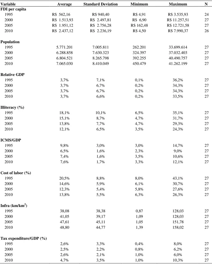
The descriptive statistics of the data are displayed in Table 4. We can notice that for the natural logarithm of FDI stock per capita, we have differents n mainly because for the first year, the BC didn’t provide the values for the states of Roraima and Rondônia. Despite the number for FDI in Sergipe in 1995 was zero, we considered it as missing mainly because the state presented a significant increase in the following years. In 2010, the FDI for Roraima wasn’t provided too.
Table 4 - Descriptive statistics of the variables (Model A) Source: the author
Variable Average Standard Deviation Minimum Maximum N
FDI per capita
1995 R$ 562,16 R$ 940,40 R$ 4,91 R$ 3.535,93 24 2000 R$ 1.513,93 R$ 2.497,81 R$ 6,90 R$ 11.257,51 27 2005 R$ 1.951,12 R$ 2.756,28 R$ 162,48 R$ 12.721,58 27 2010 R$ 2.437,12 R$ 2.236,19 R$ 4,50 R$ 7.990,37 26
Population
1995 5.771.201 7.005.811 262.201 33.699.614 27 2000 6.288.858 7.630.323 324.397 37.032.403 27 2005 6.804.521 8.265.798 392.255 40.490.757 27 2010 7.065.030 8.410.049 450.479 41.262.199 27
Relative GDP
1995 3,7% 7,1% 0,1% 36,2% 27
2000 3,7% 6,7% 0,2% 34,3% 27
2005 3,7% 6,7% 0,2% 34,3% 27
2010 3,7% 6,6% 0,2% 33,5% 27
Illiteracy (%)
1995 18,1% 10,1% 6,5% 35,1% 27
2000 15,1% 8,7% 4,7% 31,7% 27
2005 13,8% 7,7% 4,7% 29,3% 27
2010 12,1% 6,5% 3,5% 24,3% 27
ICMS/GDP
1995 9,8% 3,0% 3,0% 14,7% 27
2000 6,5% 1,6% 2,3% 9,0% 27
2005 7,4% 1,6% 3,5% 10,6% 27
2010 7,6% 1,7% 3,3% 12,1% 27
Cost of labor (%)
1995 20,5% 8,8% 8,0% 43,1% 27
2000 14,6% 5,9% 6,1% 30,7% 27
2005 12,3% 5,4% 5,8% 27,6% 27
2010 13,8% 5,5% 6,3% 26,3% 27
Infra (km/km2)
1995 38,08 38,38 0,87 128,03 27
2000 41,05 39,17 1,09 128,03 27
2005 47,61 45,11 1,05 151,78 27
2010 48,80 44,77 1,39 158,02 27
Tax expenditure/GDP (%)
1995 2,6% 3,3% 0,4% 8,0% 27
2000 2,5% 2,2% 0,8% 6,2% 27
2005 2,6% 2,1% 1,0% 6,0% 27
2010 4,7% 3,5% 1,0% 10,3% 27
value for three years – R$ 3,535.93 in 1995, R$ 11,257.51 in 2000 and R$ 7,990.37 in 2010, we have in 1995 the state of Maranhão with the lowest value R$ 4.91, Tocantins with R$ 6.90 in 2000 and Acre with R$ 4.50 in 2010. On the population variable, while we have São Paulo with more than 41 million inhabitants in 2010, Roraima had around only 450,000. Based on that, the relative GDP will follow these discrepancies with São Paulo having the highest GDP ratio, being almost 20% higher than the second placed that is Rio de Janeiro. Analyzing the illiteracy, we have São Paulo and Rio de Janeiro with one of the lowest ratio in 2010, around 4,30%, while we have the states of the Northeast region, as Alagoas and Piauí, with more than 21% of the population over 15 years being illiterate. On the ICMS/GDP ratio, we have states like Mato Grosso do Sul and Espírito Santo with the highest ratios, on average 10% for the years 2005 and 2010, and two states of the North region with the lowest ratio, about 5%. When we analyze the Northeast region on the cost of labor variable, we have Bahia with one of the lowest ratio, 6.79% in 2005 and Rio Grande do Norte with 27.55%. Thus, it shows the discrepancy not only among the Brazilian states, but also among the states from the same region. Comparing the last two variables, we have all the states from the North region with the lowest infrastructure numbers and with the highest rates of tax expenditure. Therefore, this reinforces the fact that the poorest states are those that provide more incentives in order to compensate companies for the lack of infrastructure in a general way.
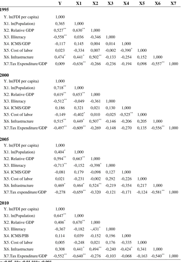
In order to verify the existence of multicollinearity among the independent variables, the Pearson correlation and the VIF (Variance Inflation Factor) were performed for all the four years, and the result are shown, respectively, in table 5 and 6 in the appendix section. Due to the absence evidence of high multicollinearity, all the variables were kept in the model.
It is important to mention that for the variables FDI per capita and the population we worked with the natural logarithm of both variables in order to reduce the strong positive asymmetry, which also reduces the variability. The transformation to natural logarithm brings linearity to the relationship of FDI with other variables.
Model B: period of 2010, 2011 and 2012
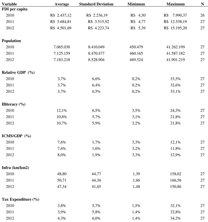
For the variable FDI per capita, the difference between both models was that in the second, the FDI data was provided in USD dollars for all the years. In this case we made the conversion, using the BC PTAX rate of the last day of each year, as we are working with the stock of FDI. For the Market size variable, the only difference was in the relative GDP, as we did not calculated the arithmetic average. Quality of workforce and Infrastructure, we used the exactly same methodology as model A. We had to exclude the variable Cost of labor due to lack of information (we only had 2010 and 2011). In the Tax burden variable in model A we used the arithmetic average of the previous five year, and in the model B, because we had the information of a short period, the ICMS collected of each state was divided by the GDP of the state for each year, without calculating the average.
Table 7 - Descriptive statistics of the variables (Model B) Source: the author
Variable Average Standard Deviation Minimum Maximum N
FDI per capita
2010 R$ 2.437,12 R$ 2.236,19 R$ 4,50 R$ 7.990,37 26 2011 R$ 3.684,81 R$ 3.515,92 R$ 4,77 R$ 12.538,19 27 2012 R$ 4.501,69 R$ 4.223,74 R$ 5,39 R$ 15.195,20 27
Population
2010 7.065.030 8.410.049 450.479 41.262.199 27 2011 7.125.159 8.470.477 460.165 41.587.182 27 2012 7.183.218 8.528.904 469.524 41.901.219 27
Relative GDP (%)
2010 3,7% 6,6% 0,2% 33,5% 27
2011 3,7% 6,4% 0,2% 32,6% 27
2012 3,7% 6,5% 0,2% 33,1% 27
Illiteracy (%)
2010 12,1% 6,5% 3,5% 24,3% 27
2011 10,8% 5,7% 3,1% 21,8% 27
2012 10,7% 5,9% 3,2% 21,8% 27
ICMS/GDP (%)
2010 7,6% 1,7% 3,3% 12,1% 27
2011 7,6% 1,6% 3,2% 11,8% 27
2012 8,0% 1,9% 3,3% 12,9% 27
Infra (km/km2)
2010 48,80 44,77 1,39 158,02 27
2011 50,71 44,36 1,66 166,58 27
2012 47,34 41,45 1,48 150,86 27
Tax Expenditure (%)
2010 3,8% 5,7% 1,5% 32,1% 27
2011 3,9% 5,8% 1,4% 32,8% 27
2012 4,3% 6,0% 1,4% 34,2% 27
3.3 Model
According to Wooldridge (2002), the analysis of panel data is used to monitor the same data during a specific period of time. In that way, it is possible to have multiple observations on the same units, allowing us to control certain unobservable characteristics of individuals, firms and, in the case of this study, the states. A second advantage of panel data is related to the fact that it allow us to study the importance of time lags in behavior or in the result of taking decisions. This information can be important since one can expect the impact on many public policies only after some time. Thus, we first perfomed the OLS (Ordinary Least Square) method and the results are presented in table 10 for model A and table 11 for model B in the appendix section.
Considering this scenario, with the description of the variables previously mentioned, the analysis on the determinants of FDI across the Brazilian states can be described as follows:
Model A
As it can be observed, the dependent variable is the natural logarithm of FDI stock per capita of a given state i at year t. The independent variables: natural logarithm of population, illiteracy, relative GDP, tax expenditure/GDP, ICMS/GDP, cost of labor and infrastructure are the explanatory variables. Then, we have the dummies for the years 2000, 2005 and 2010 to evaluate the effect of the year in the regression. The year of 1995 was used as a reference, and because of that, was excluded from the model to avoid multicollinearity.
Model B
The equation of this model is very similar with the previous one. The difference is the exclusion of the variable cost of labor, as already explained and the use of the year 2010 as the reference year. Also, we had the same result for the Hausman test: random effect.
According to Sartoris (2003), evaluating basic hypotheses about the linear regression model, ours models should have:
I. Each independent variable can not be a linear combination of the others: as shown in the tables 5 and 6 for model A nd 8 and 9 for model B, the independent variables are not highly correlated.
II. ( ) : The omission of a
relevant variable may cause autocorrelation in the erros becuase the omission of this variable puts its systematic influence in the error term, which is, supposedly, a set of non-systematic influences on the depedent variable. Thus, the autocorrelation test sugested by Wooldridge was performed for model A and the Durbin-Watson test was performed for model B, as this is applicable for shorter periods. Both did not present autocorrelation in the erros.
III. (constant): Heteroscedasticity was verified using Modified Wald test. For the FDI per capita and population variables we used the natural logarithm of these variables in both models and also worked with standard robust errors. IV. Stationary time series: the estimation of a regression model with non-stationary
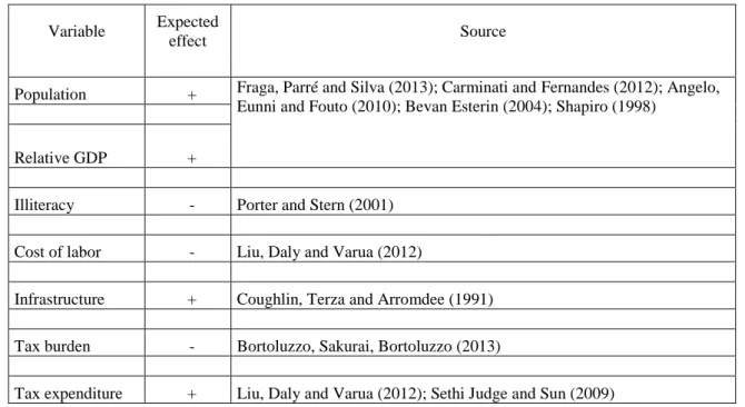
Before we present the results, based on the literature presented in all the sections of this study, below we have a table which summarizes the expected signal in the regression model and also the literature that supports it.
Table 12 – Expected effect Source: the author
Variable Expected
effect Source
Population + Fraga, Parré and Silva (2013); Carminati and Fernandes (2012); Angelo, Eunni and Fouto (2010); Bevan Esterin (2004); Shapiro (1998)
Relative GDP +
Illiteracy - Porter and Stern (2001)
Cost of labor - Liu, Daly and Varua (2012)
Infrastructure + Coughlin, Terza and Arromdee (1991)
Tax burden - Bortoluzzo, Sakurai, Bortoluzzo (2013)
4 RESULTS
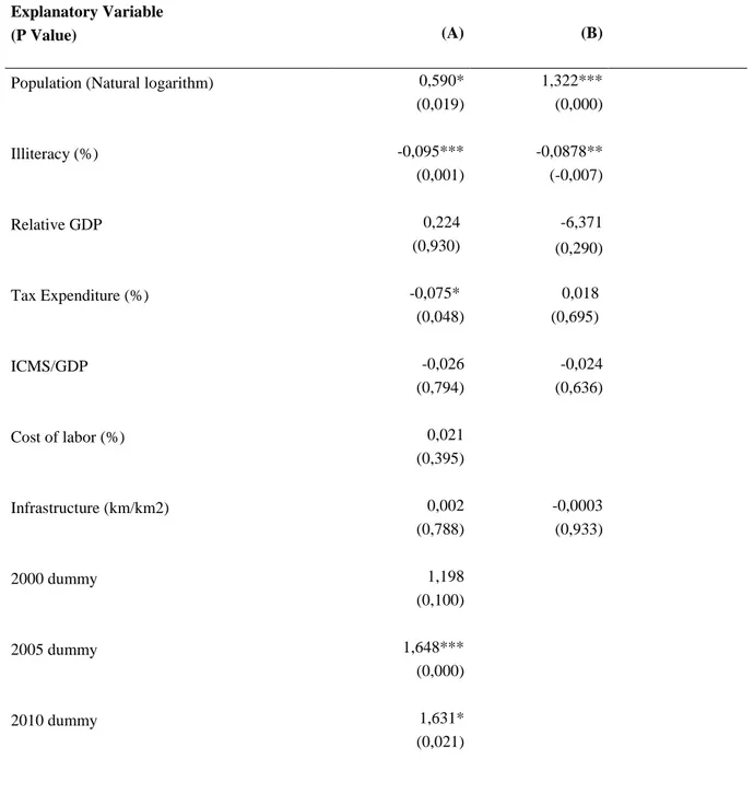
In this section we present the results of our panel regression. Table 13 reports the results of equations (A) and (B). The adjusted value of 0,624 and 0,506 respectively, further suggests that the models fit the data well. Hausman tests indicated the adequacy of random effects for the two models.
Table 7 – Results of the regression for models A and B Source: the author
Dependent Variable: ln FDI per capita
Explanatory Variable
(P Value) (A) (B)
Population (Natural logarithm) 0,590* 1,322***
(0,019) (0,000)
Illiteracy (%) -0,095*** -0,0878**
(0,001) (-0,007)
Relative GDP 0,224 -6,371
(0,930) (0,290)
Tax Expenditure (%) -0,075* 0,018
(0,048) (0,695)
ICMS/GDP -0,026 -0,024
(0,794) (0,636)
Cost of labor (%) 0,021
(0,395)
Infrastructure (km/km2) 0,002 -0,0003
(0,788) (0,933)
2000 dummy 1,198
(0,100)
2005 dummy 1,648***
(0,000)
2010 dummy 1,631*
2011 dummy 0,039 (0,607)
2012 dummy 0,296***
(0,000)
Constant -2,333 -11,56
(0,454) (0,028)
Observations 104 80
R2 0,624 0,506
Hausman Test (p-value) 0,533 0,586
* p<0,05, ** p<0,01, *** p<0,001 . Robust standard errors.
This study has found that both population and illiteracy variables have a statistically significant relationship with FDI in models A and B for the 27 different states of Brazil. The relationship between market size was a significant and positive factor in attracting FDI in all the period studied. For each 1 percent increase in the population, we will have a 0.59 percent increase in model A and 1.32 percent increase in the FDI in model B. Based on the literature previously discussed, this seems to suggest that foreign firms may be motivated to invest in Brazil under an assumption that by doing so will allow them to gain access to the Brazilian market. The state of São Paulo, which is the most populated one, is also the one with the biggest FDI inflow.
The higher the quality of labor the more attractive a region is to FDI. The results suggest a negative relation between FDI and the quality of labor: the models showed a similar number as a 1 point percent increase in the illiteracy is estimated to lead to 9.5 (model A) and 8.78 (model B) percent decrease in FDI. Again, we have São Paulo and Rio de Janeiro, the leaders of FDI inflow with the lowest illiteracy rates, around 3.67 percent.
The years were also significant in ours models. For the first model, we used the year of 1995 as a reference and the years 2005 and 2010 were positively significant. Despite the reduction of the FDI inflow in 2005, the stock more than fourfold compared to the year of reference. The reduction in 2005 was mainly driven by the exit of FDI in form of equity participation. In the year 2010, Brazil achieved a record of FDI inflow since 1995, on the amount of $ 48.4 billion dollars. One of the mais reasons for this increase was the sale of the shares of Rapsol, an oil company, to the chinese company Sinopec for $ 7.1 billion dollars. In 2012, Brazil was the country that received the third largest amount of FDI among emerging economies, with $ 65 billion dollars, only behind China ($ 120 billion) and Hong Kong ($72 billion). Although the volume was slightly below the record $ 67 billion dollars in 2011, the sare destinated to the Brazilian economy represented 4.96 percent of the world total, compared to 4.18 percent in 2011 and only 2.34 percent in 2000 (Valor Econômico). Thus, we believe that the regression captured this increase of FDI for this years.
The other variables did not meet the test of statistical significance. Actually this wasn`t expected as there is a vast literature that considers the same variables that we used as determinants for FDI. However, we believe that the specific characteristics of Brazil and the inequalities among the states explaines why other variables are not determinant. Considering the size of the country, it might not be logical to invest in the state of Acre, for example, if the region doesn’t provide you enough cosumer market and if the investors won’t find skilled labor. In this case, investing in a state like this, will only increase their costs of production, because they will have to transport the product, using an inappropriate infrastructure and they will have to scroll thorugh almost 3.500 km to reach the consumer market.
Assessing the Pearson correlation table for both models, although we have not an indication of high multicollinearity, the relative GDP and the population variables showed the highest correlation. Therefore, we decided to make a third check, alternating these variables in the models. Thus, we tested the model A with the population variable and without the relative GDP and then reversed, tested without population and with the relative GDP. The same analysis was done woth model B. The result is in the appendix section, table 14 (model A) and 15 (model B). As noticed, we had the same results as previously presentend, so we kept the models with both variables.
5 CONCLUSION
The above findings suggest that firms investing in Brazil are highly motivated by the economic performance and the potential consumer market size of the state. Thus, another important contribution of this study is related to the tax policy. Clearly, the incentives did not compensate for a weak unattractive FDI envornment. Tax is just one element among many anothers and despite all this fiscal war that we had described, it seems to not compensate for weak non-tax conditions, as the tax incentive was not determinant for the FDI inflow in the Brazilian states.
This study had similar results with Morisset and Pirnia (1999) and Devereux and Freeman (1995) that also found that incentives were not significant to determine the FDI inflow. It is also aligned with Angelo, Eunni & Fouto (2010) which the result was that the potential growth of consumer market are the most significant determinant that explains the FDI flow to Brazil.
LIMITATIONS
APPENDIX A – EXTRA TABLES
Table 5 - Pearson correlation (Model A) Source: the author
Y X1 X2 X3 X4 X5 X6 X7
1995
Y. ln(FDI per capita) 1,000 X1. ln(Population) 0,365 1,000 X2. Relative GDP 0,527** 0,630** 1,000 X3. Illiteracy -0,558** 0,036 -0,346 1,000 X4. ICMS/GDP -0,117 0,145 0,004 0,014 1,000 X5. Cost of labor 0,023 -0,334 0,007 -0,002 -0,390* 1,000
X6. Infrastructure 0,474* 0,441* 0,502** -0,133 -0,254 0,152 1,000 X7.Tax Expenditure/GDP 0,009 -0,636** -0,266 -0,236 -0,194 0,098 -0,557** 1,000
2000
Y. ln(FDI per capita) 1,000 X1. ln(Population) 0,718** 1,000 X2. Relative GDP 0,619** 0,653** 1,000 X3. Illiteracy -0,512** -0,049 -0,361 1,000
X4. ICMS/GDP 0,186 0,321 0,021 0,130 1,000 X5. Cost of labor -0,149 -0,402* 0,010 -0,025 -0,525** 1,000 X6. Infrastructure 0,515** 0,449* 0,507** -0,146 -0,206 0,205 1,000 X7.Tax Expenditure/GDP -0,497** -0,609** -0,269 -0,148 -0,270 0,135 -0,556** 1,000
2005
Y. ln(FDI per capita) 1,000 X1. ln(Population) 0,404* 1,000 X2. Relative GDP 0,594** 0,663** 1,000 X3. Illiteracy -0,713** -0,152 -0,398* 1,000 X4. ICMS/GDP -0,081 0,179 -0,098 0,127 1,000 X5. Cost of labor 0,021 -0,231 -0,002 0,292 -0,226 1,000 X6. Infrastructure 0,469* 0,464* 0,524** -0,219 -0,354 0,217 1,000 X7.Tax expenditure/GDP -0,278 -0,659** -0,320 -0,121 -0,171 -0,124 -0,581** 1,000
2010
Y. ln(FDI per capita) 1,000 X1. ln(Population) 0,647** 1,000 X2. Relative GDP 0,406* 0,670** 1,000 X3. Illiteracy -0,367 -0,182 -,431* 1,000
X4. ICMS/PIB 0,114 0,039 -0,152 0,196 1,000 X5. Cost of labor 0,005 -0,248 0,021 0,176 -0,335 1,000 X6. Infrastructure 0,308 0,441* 0,494** -0,240 -0,424* 0,341 1,000 X7.Tax Expenditure/GDP -0,552** -0,640** -0,276 -0,103 -0,068 -0,163 -0,540** 1,000 *p<0,05. **p<0,01.***p<0,001.
Table 6 – VIF (Model A) Source: the author
Explanatory Variable VIF
1995 2000 2005 2010
Population (Natural logarithm) 3,05 4,15 4,15 4,13
Relative GDP 3,05 2,91 2,82 3,08
Illiteracy (%) 1,36 1,31 1,56 1,55
ICMS/GDP 2,58 1,69 1,60 1,52
Infrastructure (km/km2) 2,70 2,41 2,93 2,71
Cost of labor 1,94 1,95 1,62 2,04
Tax Expenditure (%) 3,04 1,11 1,11 2,96
Table 8 - Pearson correlation (Model B) Source: the author
Y X1 X2 X3 X4 X5 X6
2010
Y. ln(FDI per capita) 1,000 X1. ln(Population) 0,638** 1,000 X2. Relative GDP 0,396* 0,670** 1,000 X3. Illiteracy -0,357 -0,182 -0,431* 1,000 X4. ICMS/GDP 0,058 0,028 -0,152 0,304 1,000 X5. Infrastructure 0,303 0,441* 0,494** -0,240 -0,433* 1,000 X6. Tax Expenditure 0,173 0,049 -0,021 -0,073 0,246 -0,157 1,000
2011
Y. ln(FDI per capita) 1,000 X1. ln(Population) 0,678** 1,000
X2. Relative GDP 0,412* 0,676** 1,000 X3. Illiteracy -0,375 -0,185 -0,443* 1,000 X4. ICMS/GDP 0,103 0,121 -0,069 0,206 1,000 X5. Infrastructure 0,280 0,368 0,453* -0,207 -0,358 1,000 X6. Tax Expenditure 0,186 0,052 -0,021 -0,095 0,242 -0,177 1,000
2012
Y. ln(FDI per capita) 1,000 X1. ln(Population) 0,603** 1,000 X2. Relative GDP 0,399* 0,675** 1,000 X3. Illiteracy -0,347 -0,137 -0,419* 1,000
X4. ICMS/GDP 0,116 0,053 -0,180 0,299 1,000 X6. Infrastructure 0,267 0,394* 0,495** -0,178 -0,315 1,000 X7. Tax Expenditure 0,174 0,059 -0,019 -0,086 0,225 -0,167 1,000