Do Options Contain Information About
Excess Bond Returns?
∗
Caio Almeida
†Jeremy J. Graveline
‡Scott Joslin
§First Draft: June 3, 2005
Current Draft: November 18, 2005
COMMENTS WELCOME
PLEASE DO NOT CITE WITHOUT PERMISSION
Abstract
There is strong empirical evidence that risk premia in long-term interest rates are time-varying. These risk premia critically depend on interest rate volatility, yet existing research has not examined the im-pact of time-varying volatility on excess returns for long-term bonds. To address this issue, we incorporate interest rate option prices, which are very sensitive to interest rate volatility, into a dynamic model for the term structure of interest rates. We estimate three-factor affine term structure models using both swap rates and interest rate cap prices. When we incorporate option prices, the model better captures interest rate volatility and is better able to predict excess returns for long-term swaps over short-term swaps, both in- and out-of-sample. Our results indicate that interest rate options contain valuable infor-mation about risk premia and interest rate dynamics that cannot be extracted from interest rates alone.
∗We thank Chris Armstrong, Snehal Banerjee, David Bolder, Darrell Duffie, Yaniv
Kon-chitchki, and seminar participants at Stanford GSB graduate student seminar for helpful comments. We are very grateful to Ken Singleton for many discussions and comments.
†Ibmec Business School,calmeida@ibmecrj.br
Introduction
In a regression framework, Fama and Bliss (1987) demonstrate that expected excess bond returns are both predictable and time-varying. Campbell and Shiller (1991) present further evidence from regressions that risk premiums on long-term bonds are also time varying. Recently, Duffee (2002) and Dai and Singleton (2002) have shown that dynamic term structure models with a flexible specification of the market price of interest rate risk can capture this variation in expected returns. However, the expected excess returns for long-term bonds depends on both the price of interest rate risk as well as the amount of interest rate volatility, yet comparatively little research attention has been focused on the impact of time-varying volatility on expected excess returns.
With few exceptions, previous research has not included interest rate op-tions when estimating dynamic term structure models and therefore has not exploited the additional information about interest rate volatility that may be contained in these option prices. In this paper we estimate arbitrage-free dynamic term structure models jointly on both swap rates and the prices of interest rate caps. We use quasi-maximum likelihood to estimate three-factor affine term structure models with 0, 1, or 2 factors having stochastic volatil-ity.1 In order to make estimation with cap prices computationally feasible, we build on the work of Jarrow and Rudd (1982) and develop a
computa-1
See Dai and Singleton (2000) for a detailed specification of the AM(N) affine term
tionally efficient method for computing cap prices that is well-suited to esti-mation. When we incorporate information in option prices, we significantly improve the model’s ability to price interest options without impairing its ability to capture the term structure of interest rates. More importantly, the model’s that are estimated with options are dramatically better at predict-ing excess returns for long-term swaps over short-term swaps, both in- and out-of-sample.
Previous papers that have used both interest rates and interest rate op-tions in estimation have focused on accurately pricing both interest rates and options. Umantsev (2002) estimates affine models jointly on both swaps and swaptions and analyzes the volatility structure of these markets as well as factors influencing the behavior of interest rate risk premia. Longstaff et al. (2001) and Han (2004) explore the correlation structure in yields that is required to simultaneously price both caps and swaptions. Bikbov and Cher-nov (2004) use both Eurodollar futures and option prices to estimate affine term structure models and discriminate between various volatility specifica-tions. Our paper differs from these papers in that we examine how including options in estimation affects a model’s ability to capture the dynamics of interest rates and predict excess returns.
of conditional volatility. Section 5 compares the estimated models’ ability to predict excess returns and Section 6 concludes. Technical details, and all tables and figures are contained in the appendix.
1
Excess Returns in Fixed Income Markets
Any bond held for a period less than its maturity will have a risky return. For example, although the year interest rate is known, the return on a 5-year bond that is sold in one 5-year is uncertain and risky. Economic reasoning suggests that investors may demand a premium for holding this risk. Interest rate volatility is one measure of the amount of such risk that a bond is exposed to, and in this section we use regression analysis to test whether interest rate volatility explains variation in bond returns.
Specifically, defining:
pnt = price at time t of n year zero coupon bond,
rnt = n-year continuously compounded yield
= −1
nlog(p
n t).
The log excess return for holding an n-year bond for one year is then:
rte,n+1 = log(pn−1
t+1)−log(pnt)−rt1
= −(n−1)rn−1
t+1 +nr
Previous papers have shown that the current term structure of interest rates can be used to predict excess bond returns. For instance, Fama and Bliss (1987) and Campbell and Shiller (1991) provide evidence that the slope of the yield curve explains variation in excess returns. Cochrane and Piazzesi (2005) argue that the entire yield curve provides valuable information for explaining variation in risk premia.
If investors demand a premium for holding long term bonds with a risky return, then interest rate volatility may provide additional predictive power in a regression. As a measure of volatility, we use interest rate cap data. An interest rate cap is a financial derivative that caps the interest rate that is paid on the floating side of a swap. The market convention is to quote prices in terms of the volatility implied by Black’s formula. In our regression analysis, we use the Black implied volatility of at-the-money caps as a measure of the unobserved true volatility.2 The implied volatility from at-the-money caps provides a forward looking measure of volatility that incorporates risk preferences.
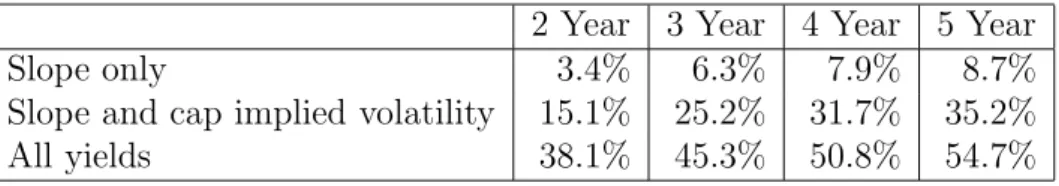
As a preliminary test of this hypothesis, we regress the one year excess returns of 2- to 5-year bonds on three sets of explanatory variables (all include a constant):
1. the slope of the yield curve, taken as rn t −rt1,
2. the slope andn-year interest rate cap implied volatility,
3. one to five year zero rates.
We report the R2 from the regressions using 483 weekly observations from June 1995 to March 2004 in Table 1. The results indicate that indeed in-cluding the cap implied volatility increases the amount of variation which is explained from just using the slope alone. However, it should be noted that the sample size is relatively small and the regressions choose coefficients to maximize the R2 by construction (in particular there are only 10 non-overlapping one year returns.)
The preliminary evidence in these regressions indicates that excess bond returns depend on interest rate volatility, and suggests that it may be benefi-cial to incorporate interest rate cap prices into a dynamic model of the term structure of interest rates. We now turn to this objective.
2
Model and Estimation Strategy
Empirical studies of dynamic asset pricing models estimate the dynamics of a pricing kernel Mtthat prices at timet an arbitrary paymentZT at timeT by
Et[(MT /Mt)ZT]. Dynamic term structure models focus particular attention
on pricing payoffs at different maturities T.
The dynamic term structure models we estimate fall within the broad class of models in which the pricing kernel is modelled as
dMt = −Mtr(Xt)dt−MtΛ (Xt)
where Xt are latent factors with dynamics
dXt = µ(Xt)dt+σ(Xt)dWt.
The price PT
t at time t of zero coupon bond3 that pays $1 at time T is
Et[MT / Mt] and depends critically on the dynamics of both the
instanta-neous short interest ratert =r(Xt) and the market price of risk Λt= Λ (Xt).
A simple application of Itˆo’s Lemma implies that zero coupon bond price dy-namics follow
dPT
t =
rtPtT +
∂PT t
∂Xt ·
σtΛt
dt+∂P
T t
∂Xt ·
σtdWt.
From (1) it is clear that expected excess returns of zero coupon bonds depend on both the market price of risk Λt as well as the volatility σt of the latent
factors.
We estimate three 3-factor affine term structure models4 such that:
rt = ρ0+ρ1·Xt,
µP
t = K
P
0 +K1P Xt,
σtσ
′
t = H0+H1·Xt
3In this paper we focus on modelling the swap rate and therefore the price of a zero
coupon bond is the price of $1 discounted at the relevant swap discount rate for that maturity.
4These models were introduced by? and Dai and Singleton (2000). We use an extended
The drift is also affine under the risk neutral measure:
µQt = K
Q
0 +K
Q
1 Xt
and the associated market price of risk is given by:
Λ (Xt) = (σt)
−1h
K0P −K0Q+K1P −K1QXt
i
Any claim with payoff at time T given by f(XT) can then be priced by
the discounted risk-neutral expected value
EtQ[e
−RT
t rτdτf(X
T)]
In this affine setting, Duffie and Kan (1996) show that zero coupon bond prices are given by
PT (Xt, t) = eA(T
−t)+B(T−t)·Xt,
where the functions A and B satisfy Riccati ODEs
˙
B = −ρ1 +KQ
⊤
1 B+ 1 2B
⊤
H1B , B(0) = 0,
˙
A = −ρ0 +KQ
⊤
0 B+ + 1 2B
⊤
H0B , A(0) = 0.
An interest rate cap is a financial derivative that caps the interest rate that is paid on the floating side of a swap. And so a cap is a portfolio of options on 3 month LIBOR. The priceCN
t C
of anN-period interest rate cap with strike rate C and time ∆t between floating interest payments is5
CN
t C
=
N
X
n=2 Et
"
e−Rtn∆t
t rτdτ 1
Pt+n∆t t+(n−1)∆t
− 1 +C∆t
!+#
.
In the setting of affine term structure models, Duffie et al. (2000) show that cap prices can be computed as a sum of inverted Fourier transforms. However, as we show in the appendix, when the solutions A and B to the Riccati ODEs are not known in closed form, numerical evaluation of the in-verted Fourier transforms is computationally expensive for use in estimation. We use a more computationally efficient cumulant expansion technique to compute cap prices.6 The cumulant expansion method we develop is espe-cially well-suited to option pricing in an affine framework and is described in more detail in Section C in the appendix.
Our data, obtained from Datastream, consists of Libor, swap rates, and at-the-money cap implied volatilities from January 1995 to March 2004. We use 3-month Libor and the entire term structure of swap rates to bootstrap swap zero rates at 1-, 2-, 3-, 5- and 10-years.7 Finally, we use at-the-money
5The market convention is that there is no cap payment for the first floating rate
payment.
6Jarrow and Rudd (1982) were the first to use cumulant expansions in an asset
pric-ing settpric-ing. Collin-Dufresne and Goldstein (2002) use cumulant expansions to compute swaption prices.
caps with maturities of 1-, 2-, 3-, 4-, 5-, 7-, and 10-years.
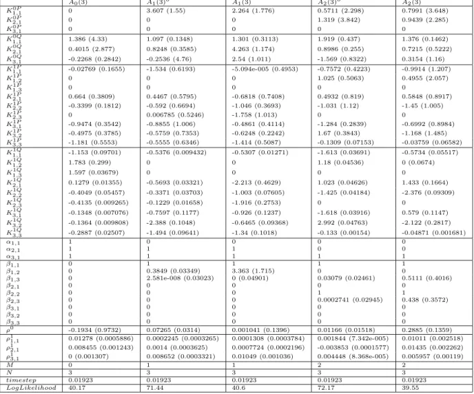
We use quasi-maximum likelihood to estimate model parameters forA0(3),
A1(3), and A2(3) models.8 The full model specifications and estimation pro-cedure are described in detail in the appendix. All of the models are esti-mated using the assumption that the model correctly prices 3-month Libor and the 2- and 10-year swap zero coupon rate exactly and the remaining swap zero coupon rates are assumed to be priced with error.9 For theA
1(3)o and A2(3)o models, we also assume that at-the-money caps with maturities of 1-, 2-, 3-, 4-, 5-, 7-, and 10-years are priced with error. For each model, we used the following procedure to obtain Quasi-maximum likelihood estimates:
1. Randomly generate 25 feasible sets of starting parameters.
2. Starting from the best of the feasible seeds, use a gradient search method to obtain a (local) maximum of the quasi-likelihood function constructed using the model’s exact conditional mean and variance.10
3. Repeat these steps 1000 times to obtain a global maximum.
The parameter estimates are contained in Table 2. observations.
8An
AM(3) model has three latent factors withM factors having stochastic volatility.
9By assuming that a subset of securities are priced correctly by the model, we can use
these prices to invert for the values of the latent states. See Chen and Scott (1993) for more details.
10In an affine model, the conditional mean and variance are known in closed form as the
3
Cross Sectional Fit
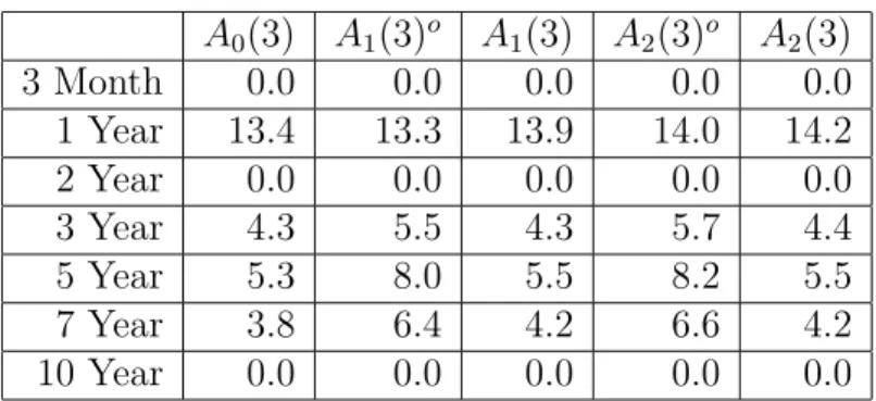
Table 3 provides the root mean squared errors (in basis points) for the swap zero coupon rates. The root mean squared errors are 0 for the 3-month, 2-, and 10-year swap zero rates because the latent states variables are chosen so that the models correctly price these instruments. The A0(3) model has the lowest mean squared errors across term structure maturities. More impor-tantly, the pricing errors are only slightly higher for the A1(3)o and A2(3)o
models that are estimated with options than they are for theA1(3) andA2(3) models that are not estimated with options. Thus, including options in esti-mation does not appear to adversely affect the model’s ability to successfully price the cross-section of interest rates.
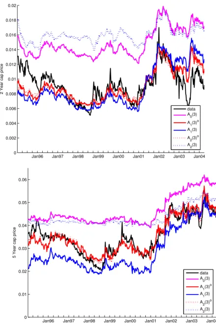
Figure 1 plots at-the-money cap prices and Table 4 displays the root mean squared error in percentage terms for at-the-money caps with various matu-rities. While theA0(3) model had the lowest pricing errrors for interest rates, it has the highest pricing errors for caps. The large cap pricing errors for the
A0(3) model are due to its lack of factors with stochastic volatility. Since the
A0(3) model does not contain stochastic volatility, we do not estimate it with
options. The cap pricing errors for the A1(3)o model are approximately half
the term structure of swap zero rates, it dramatically decreases the pricing errors for interest rate caps.11
4
Matching Volatility
For theA1(3)oand A2(3)o models, cap prices are used in estimation and thus
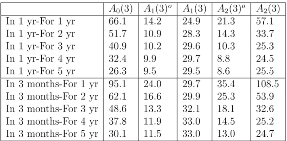
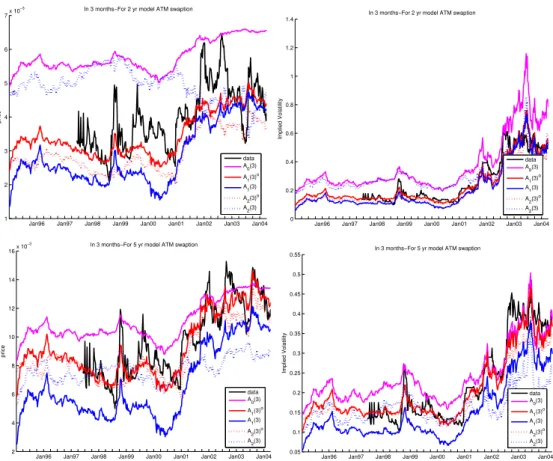
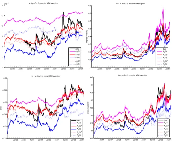
it is possible that these models are accurately capturing cap prices without accurately capturing interest rate volatility. As an additional measure of how well the models are capturing interest rate volatility, we also compute the prices of at-the-money swaptions. Swaptions differ from interest rate caps in that they are a single option on a long maturity swap rate rather than a portfolio of options on the 3-month Libor interest rate.
Figures 2 and 3 plot the times series of Black’s swaption implied volatil-ities.12 Tables 5 and 6 give the pricing errors for a cross section of swaption prices. The results for swaptions are similiar to those for caps. The A0(3) model has the largest pricing errors. Again, the swaption pricing errors for the A1(3)o and A2(3)o models that are estimated with caps are significantly
lower than their counterpart models A1(3) and A2(3) that are estimated without using options. Data from SwapPX indicates that typical bid-ask
11It should be noted that none of the five models does a good job of pricing 1-year caps.
Dai and Singleton (2002) find that a fourth factor is required to capture the short end of the yield curve. We choose to implement more parsimonious three-factor models because we are primarily interested in predicting changes in long term yields.
12
spreads are on the order of 2% implied volatility. Thus, the pricing errors for the A1(3)o and A2(3)o models are very close to the bid-ask spreads in these
markets. Thus we find that these models are able to capture prices in both the bond and cap and swaptions markets (with the exception of the short end of the curve.)
In regards to pricing, these results differ somewhat from prior literature. Longstaff et al. (2001) and Han (2004) suggest that affine term structure models require a large number of parameters to simultaneously match both swaption and cap prices. Longstaff et al. (2001) price swaptions in estimation and find implied errors on cap prices of a similar magnitude to ours, but which under-price the caps on average whereas our model estimates have near zero average price errors for both cap and swaptions. Jagannathan et al. (2003) find that AN(N) models with independent factors do a very poor job of
pricing caps whether or not they are included in the estimation. However, we use a more general price of risk and our computational procedure allows us to include affine models where cap prices are not known in closed form.
Our results are similar to Umantsev (2002) and Joslin (2005). Umantsev (2002) finds that low factor affine models can simultaneously price well both a cross section bonds and swaptions (though he does not consider caps.) Joslin (2005) finds the complementary result that including swaption prices in estimation gives models which price bonds, swaptions, and caps well.
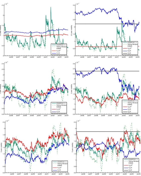
volatility however is not observed. For estimates of conditional volatility based on historical data we use a 26 week rolling window, an exponential weighted moving average (EWMA) with a 26-week half-life, and estimate an EGARCH(1,1) for each maturity.
Figures 4 plots the model’s conditional volatility of zero coupon rates against these estimates of conditional volatility using historical data. None of the models do a good job of tracking the various estimates of the volatility of the 6-month zero coupon rate, though the A1(3)o and A2(3)o at least appear to get the level right.13 However, for the 2- and 5- year maturities, the conditional volatility of theA1(3)oandA2(3)omodels more closely tracks the
various estimates of conditional volatility. The A2(3) model complete misses the level of volatility for the 6-month and 2-year zero coupon rates. Though, on average, the A2(3) model matches the level of the volatility of the 5-year zero coupon rate, it appears to miss the dynamics. The A1(3) model does a better job than the A2(3) model at matching the various historical estimates of conditional volatility. However, in each case, the A1(3) andA2(3) models are worse than their A1(3)o and A
2(3)o counterparts.
13
5
Predictability of Excess Returns
Table 7 presents evidence on the predictability of excess returns for long term interest rates for the in-sample period from January 1995 to March 2004. R2’s are calculated as
R2 = 1−var(Rexpectedt,n −Rt,tn+1)/var(Rnt,t+1),
where where var(.) denotes variance, Rexpectedt,n are weekly model implied
expected returns for discount bonds with nyears to maturity, and Rn t,t+1 are weekly realized returns for the corresponding bond. We includeR2’s for each model we estimated, as well as R2’s from three versions of the regressions of excess returns on forward rates as performed in Cochrane and Piazzesi (2005).14
On average, amongst models that were estimated without options, the
A0(3) model has higher excess return predictability than the A1(3) model,
which in turn has higher predictability than the A2(3) model. Both Duffee (2002) and Dai and Singleton (2002) also estimate three-factor term structure
14For different maturities, Cochrane and Piazzesi (2005) run regressions of yields
vari-ations on a linear combination of forward rates. Letting pn
t and ynt denote respectively
the price and yield to maturity of a n-year discount bond at time t, for each fixed nthey regress:
rn
t+1−y 1
t =β n
0 +β
n
1y 1
t+β n
2f 2
t +β n
3f 3
t +β n
4f 4
t +β n
4f 5
t +ǫ n t+1,
where rn
t+1 is the holding period return from buying annperiod discount bond at timet
and selling it at timet+ 1, andfi t =p
i−1
t −pit, i= 2, ...,5 is the timetone period forward
rate for loans between the maturitiesi−1 andi. CP5are the regressions described above,
while CP10are correspondent regressions using one period forward rates for loans between
maturities that go up to 10 years. Finally, CP5,10use only 5 one year forward rates (which
models without options and find that the A0(3) model has the best perfor-mance in terms of predictability. When options are included in estimation, the predictability of both theA1(3)oandA2(3)omodels improve dramatically over theirA1(3) andA2(3) counterparts. On average, the R2’s for theA1(3)o
model are two to three times as large as those for the A0(3). The difference is dramatic for the 10-year maturity were the R2 for theA
0(3) model is only 2.5% but the R2 for the A
1(3)o is 33.1%.
Moreover, the R2’s are much closer in magnitude to those obtained from the regressions in Cochrane and Piazzesi (2005). The regressions in Cochrane and Piazzesi (2005) are designed to only match excess returns and so they serve as somewhat of an upper bound for the the level of predictability of excess returns.
Table 8 provides R2’s for the out-of-sample period from April 1988 to December 1994. (Recall that the models were estimated with historical data from January 1995 to March 2004, which corresponded to the availability of cap data in Datastream.) The A0(3) and A2(3) models do extremely poorly out-of-sample, whileCP10seems to be overfitting in-sample data (which mo-tiviating including the CP5,10). As was the case with in-sample
predictabil-ity, the inclusion of options in the A1(3)o and A2(3)o models dramatically
improves their sample predictability. Equally as striking, the out-of-sample predictability of the A1(3)o model estimated with options is on par
Figure 5 plots the realized excess returns as well as the expected excess returns for the A0(3), A1(3), and A1(3)o models and the CP5 regressions. The variation in expected excess returns is higher for the A1(3)o and A2(3)o
models than for their A1(3) and A2(3) counterparts, presumably because these models capture more time variation in volatility when they are esti-mated with options. The results in Table 9 confirm this observation. In addition, not only is the level of predictability of excess returns higher for the A1(3)o and A2(3)o models than for the A0(3) model, the variation in the predict excess returns is actually lower. Since there is no time variation in volatility for the A0(3) model, all of the variation in expected excess returns is due to variation in the market price of risk. Thus, the A0(3) model ap-pears to overstate the true amount of variation in the market prices of risk. The variation in expected excess returns for theA1(3)o and A2(3)o models is also lower than that for the CP5 regressions. However, the CP5 regression is not an economic model and therefore the expected excess returns cannot be decomposed into volatility and the market prices of risk.
6
Conclusion
structure of interest rates. Furthermore, the model’s that are estimated with options are dramatically better at predicting excess returns for long-term swaps over short-term swaps, both in- and out-of-sample. In contrast to previous literature, the arbitrage-free models with the most predictive power contain a stochastic volatility component. Our results indicate that inter-est rate options contain valuable information about term structure dynamics that cannot be extracted from interest rates alone.
References
Ruslan Bikbov and Mikhail Chernov. Term structure and volatility: Lessons from the eurodollar markets. Working Paper, 7 June 2004.
Fischer Black. The pricing of commodity contracts. Journal of Financial
Economics, 3(1-2):167–179, January-March 1976.
John Y. Campbell and Robert J. Shiller. Yield spreads and interest rate movements: A bird’s eye view. Review of Economic Studies, 58(3):495– 514, May 1991.
Ren-Raw Chen and Louis Scott. Maximum likelihood estimation for a mul-tifactor equilibrium model of the term structure of interest rates. Journal
of Fixed Income, 3:14–31, 1993.
risk specifications for a ne models: Theory and evidence. Working Paper, Princeton University, 15 October 2004.
John H. Cochrane and Monika Piazzesi. Bond risk premia. American
Eco-nomic Review forthcoming, 2005.
Pierre Collin-Dufresne and Robert S. Goldstein. Pricing swaptions within an affine framework. Journal of Derivatives, 10(1):1–18, Fall 2002.
Pierre Collin-Dufresne, Robert S. Goldstein, and Christopher S. Jones. Can the volatility of interest rates be extracted from the cross section of bond yields? an investigation of unspanned stochastic volatility. Working Paper, 5 August 2004.
Qiang Dai and Kenneth J. Singleton. Specification analysis of affine term structure models. Journal of Finance, 55(5):1943–1978, October 2000.
Qiang Dai and Kenneth J. Singleton. Expectation puzzles, time-varying risk premia, and affine models of the term structure. Journal of Financial
Economics, 63(3):415–441, March 2002.
Gregory R. Duffee. Term premia and interest rate forecasts in affine models.
Journal of Finance, 57(1):405–443, February 2002.
J. Darrell Duffie, Jun Pan, and Kenneth Singleton. Transform analysis and asset pricing for affine jump-diffusions. Econometrica, 68(6):1343–1376, November 2000.
Eugene F. Fama and Robert R. Bliss. The information in long-maturity for-ward rates. American Economic Review, 77(4):680–692, September 1987.
Bin Han. Stochastic volatilities and correlations of bond yields. Working Paper, October 2004.
Ravi Jagannathan, Andrew Kaplin, and Steve Sun. An evaluation of multi-factor cir models using libor, swap rates, and cap and swaption prices.
Journal of Econometrics, 116(1-2):113–146, September-October 2003.
Robert Jarrow and Andrew Rudd. Approximate option valuation for arbi-trary stochastic processes. Journal of Financial Economics, 10(3):347–369, November 1982.
Scott Joslin. Completeness in fixed income markets. 2005. Working Paper, Stanford University.
Francis A. Longstaff, Pedro Santa-Clara, and Eduardo S. Schwartz. The relative valuation of caps and swaptions: Theory and empirical evidence.
Journal of Finance, 56(6):2067–2109, December 2001.
Len Umantsev. Econometric Analysis of European Libor-Based Options
A
Detailed Model Specifications
The short rate is given by rt = ρ0 +ρ1 ·Xt, where Xt is a Markov state
variable with dynamics and the physical and risk neutral measures given by:
dXt = (K0P +K1PXt) +σtdBtP
dXt = (K0Q+K1QXt) +σtdBtQ
and where the conditional variance is affine in the state: σtσ
′
t=H0+H1·Xt.
In the A0(3) model, H1 ≡ 0, so none of the three factors in Xt have
stochastic volatility. In the A1(3) model, one of the factors in Xt drives
stochastic volatility, and in the A2(3) model, two of the factors in Xt drive
A
0(3)
Model Specification
K1P =
KP
1,11 0 0
KP
1,21 K1P,22 0
KP
1,31 K1P,32 K1P,33
K0P =
0 0 0
σt = I3
ρ1,1 ≥ 0, ρ1,2 ≥0, ρ1,3 ≥0
A
1(3)
Model Specification
KP 1 = KP
1,11 0 0
KP
1,21 K1P,22 K1P,23
KP
1,31 K1P,32 K1P,33
KP 0 = KP
0,1 0 0
K1Q =
K1Q,11 0 0
K1Q,21 K
Q
1,22 K
Q
1,23
K1Q,31 K1Q,32 K1Q,33
K0Q=
K0Q,1
0 0
σt =
p X1
t 0 0
0 p1 +β12Xt1 0
0 0 p1 +β13Xt1
KP
0,1 ≥ 1 2, K
Q
0,1 ≥ 1 2
β12 ≥ 0, β13 ≥0
A
2(3)
Model Specification
K1P =
KP
1,11 K1P,12 0
KP
1,21 K1P,22 0
KP
1,31 K1P,32 K1P,33
K0P =
KP
0,1
KP
0,2 0
K1Q =
K1Q,11 K
Q
1,12 0
K1Q,21 K
Q
1,22 0
K1Q,31 K
Q
1,32 K
Q
1,33
K0Q =
K0Q,1
K0Q,2
0
σt =
p X1
t 0 0
0 pX2
t 0
0 0 p1 +β13Xt1 +β23Xt2
K0P,1 ≥ 1 2, K
P
0,2 ≥ 1 2, K
Q
0,1 ≥ 1 2, K
Q
0,2 ≥ 1 2
KP
1,12 ≥ 0, K1P,21 ≥0, K
Q
1,12≥0, K
Q
1,21 ≥0
β13 ≥ 0, β23≥0
ρ1,3 ≥ 0
B
Detailed Estimation Procedure
We estimate all the models using quasi-maximum likelihood in a procedure similar to Duffee (2002) and Dai and Singleton (2002). Using the instruments priced without error and the risk neutral dynamics of Xt, we invert to find
implied prices of the instruments priced without error. Following Dai and Singleton (2002), we assume that the pricing errors are i.i.d. normal with mean zero. Finally, using the physical dynamics of the state vector and the QML approximation, we compute the likelihood of the inverted states. This gives the liklelihod of a given set of parameters to be:
likelihood =YℓP
QM L(Xt|Xt−1)·(Jacobian)·(likelihood of pricing errors)
We use a slighlty different procedure than Duffee (2002) to compute the conditional mean and variance of the state variable. For a general affine process, Xt, with conditional driftK0+K1Xt and conditional varianceH0+
H1·Xt, the mean and variance ofXtconditional onX0satisfy the differential equations
˙
Mt = K0+K1Mt
˙
Vt = K1Vt+VtK1t+H0+H1·Mt
If we letfbe the (N+N2)-vector (M,vec(V)), then by stacking these coupled ODEs we see that f satisfies the ODE
˙
f =
K1 0
∆ IN ⊗K1 +K1⊗IN
f +
K0
vec(H0)
Where ∆ is an (N2×N) matrix with ∆
con-sidering separate cases to solve this ODE in closed form, we instead compute the fundamental solution numerically using 4th order Runge-Kutta. From the fundamental solution, it is then easy to compute the solution for arbitrary initial conditions.
C
Cap Valuation via a Cumulant Expansion
Recall that PT
t is the price at timet of $1 paid at timeT. The priceCtN C
of an N-period interest rate cap with strike rate C and time ∆t between floating interest payments is
CN
t C
=
N
X
n=2 Et
"
Mt+n∆t
Mt
1
Ptt+(+nn−∆1)∆t t
− 1 +C∆t
!+#
= e−A(∆t)
N
X
n=2
Gt −A(∆t)−ln 1 +C∆t
;−B(∆t), B(∆t),(n−1) ∆t
−e−A(∆t) 1 +C∆t
N
X
n=2
Gt −A(∆t)−ln 1 +C∆t
; 0, B(∆t),(n−1) ∆t ,
where
Gt(y;b, γ, τ) := Et
Mt+τ
Mt
eb⊤Xt+τ γ⊤X
t+τ ≤y
.
By the L´evy inversion formula,
Gt(y;b, γ, τ) =
1
2Gˆt(0;b, γ, τ)− 1
π
Z ∞
0 1
v Im
h
e−i v yˆ
Gt(v;b, γ, τ)
i
dv ,
where ˆGt is the Fourier transform of Gt. In an affine framework ˆGt is given
by
ˆ
Gt(v;b, γ, τ) = Et
Mt+τ
Mt
e(b+ivγ)⊤Xt+τ
= eA(b+ivγ,τ)+B(b+ivγ,τ)⊤Xt,
where, A and B satisfy the Riccati ODEs
∂ B(b+ivγ, u)
∂ u = −ρ1+K
Q⊤
1 B(b+ivγ, u) + 1
2β∆ [B(b+ivγ, u)]B(b+ivγ, u) ,
∂ A(b+ivγ, u)
∂ u = −ρ0+K
Q⊤
0 B(b+ivγ, u) + 1 2α
⊤
∆ [B(b+ivγ, u)]B(b+ivγ, u) ,
with boundary conditions
B(b+ivγ,0) = b+ivγ ,
A(b+ivγ,0) = 0.
L´evy inversion formula is not computationally feasible for model estimation. Instead, we use a more computationally efficient cumulant expansion tech-nique to compute cap prices. The cumulant expansion requires that we com-pute the Taylor series expansion of the log of the Fourier transform of Gt.
Define the cumulants cm by
cm :=
∂mln ˆG
t(0;b, γ, τ)
∂(iv)m
= i3m
(
∂mA(b+ivγ, τ)
∂ vm
| {z }
∂m v A(τ)
+∂
mB(b+ivγ, τ)⊤ ∂ vm
| {z }
∂m vB(τ)
Xt
)
v
=0
,
so that
ln ˆGt(v;b, γ, τ) = ln ˆGt(0;b, γ, τ) +
∞
X
m=1 1
m!cm(iv)
m
.
In an affine framework, the cumulants are affine in the state vector Xt
with coefficients that again satisfy Riccati ODEs,
∂v1B(u) = K
Q⊤
1 ∂v1B(u) +β∆
h
B(u)⊤ΣiΣ⊤
∂v1B(u) , ∂v1B(0) =iγ ,
∂v1A(u) = K
Q⊤
0 ∂v1B(u) +α
⊤
∆hB(u)⊤ΣiΣ⊤
and for m >1,
∂vmB(u) = K
Q⊤
1 ∂
m
v B(u) + m
X
k=0
ϕmkβ∆
h
∂m−k
v B(u)
⊤
ΣiΣ⊤
∂vkB(u) , ∂ m
v B(0) = 0,
∂m
v A(u) = K
Q⊤
0 ∂mv B(u) + m X k=0 ϕm kα ⊤
∆h∂m−k
v B(u)
⊤
ΣiΣ⊤ ∂k
vB(u), ∂vmA(0) = 0,
where ϕm
k =
m
k
if m6= 2k and ϕm k = 12
m
k
if m= 2k.
Once we have computed the cumulants, we can accurately approximate
Gt by
Gt(y;b, γ, τ) ≈ M
X
m=0
χm
−1Φ−1(y−c1) +χm0 Φ0(y−c1)
where
Φ−1(y) =
1
√
2πc2
e−y 2 2c2
Φ0(y) =
Z y
−∞
Φ−1(z) dz ,
and the coefficients χm
−1 and χm0 are related to the cumulants as described
below. Φ−1 and Φ0 are just the density and cumulative distribution of the
Normal distribution. There exist accurate approximations to the cumulative Normal density, therefore computation of cap prices using a cumulant expan-sion does not require any numerical integration (aside from solving Riccati ODEs). We now turn to determining the coefficients χm
Define am to be the coefficients in a Taylor series expansion of
ˆ
Gt(v;b, γ, τ) e
−[c1(iv)+1 2c2(iv)
2] ,
about v = 0, so that
ˆ
Gt(v;b, γ, τ) = ec1(iv)
−1 2c2v2
∞
X
m=0
amvm.
Then
1 2π
Z ∞
−∞
e−i z vˆ
Gt(v;b, γ, τ)dv =
∞ X m=0 am 1 2π Z ∞ −∞
e−i(z−c1)v−12c2v2vmdv
= ∞ X m=0 am 1 2π Z ∞ −∞
∂meuv−1 2c2v2
∂um
u=−i(z−c1) dv = ∞ X m=0 ∂m ∂um am 1 √
2πc2
eu 2 2c2
u=−i(z−c1)
≈ M X m=0 ∂m ∂um am 1 √
2πc2
eu 2 2c2
u=−i(z−c1)
=: √1
2πc2
e−(
z−c1)2
2c2
M
X
m=0
λm(z−c1)m ,
Then by the inverse Fourier transform,
Gdt(y;b, γ, τ) =
Z y
−∞
1 2π
Z ∞
−∞
e−i z vˆ
Gdt (v;b, γ, τ)dv dz
≈ M
X
m=0
λm
Z y
−∞
1
√
2πc2
e−(
z−c1)2
2c2 (z−c1)mdz
| {z }
Φm(y−c1)
,
Φm(y) can be expressed in terms of Φ−1(y) and Φ0(y) via the recursive
relationship
Φ−1(y) =
1
√
2πc2
e−y 2 2c2
Φ0(y) =
Z y
−∞
Φ−1(z) dz ,
Φm(y) = −c2
Z y
−∞
zm−1dΦ−1(z)
= −c2
ym−1
Φ−1(y)−(m−1) Φm−2(y)
.
Therefore, Gt(y;b, γ, τ) is of the form
Gt(y;b, γ, τ) ≈ M
X
m=0
χm−1Φ−1(y−c1) +χm0 Φ0(y−c1)
,
as desired.
2 Year 3 Year 4 Year 5 Year
Slope only 3.4% 6.3% 7.9% 8.7%
Slope and cap implied volatility 15.1% 25.2% 31.7% 35.2%
All yields 38.1% 45.3% 50.8% 54.7%
Table 1: Regression of Excess Returns.
A0(3) A1(3)o A1(3) A2(3)o A2(3)
K0P
1,1 0 3.607 (1.55) 2.264 (1.776) 0.5711 (2.298) 0.7991 (3.648)
K20P,1 0 0 0 1.319 (3.842) 0.9439 (2.285)
K0P
3,1 0 0 0 0 0
K10Q,1 1.386 (4.33) 1.097 (0.1348) 1.301 (0.3113) 1.919 (0.437) 1.376 (0.1462)
K20Q,1 0.4015 (2.877) 0.8248 (0.3585) 4.263 (1.174) 0.8986 (0.255) 0.7215 (0.5222)
K30Q,1 -0.2268 (0.2842) -0.2536 (4.76) 2.54 (1.011) -1.569 (0.8322) 0.3154 (1.16)
K1P
1,1 -0.02769 (0.1655) -1.534 (0.6193) -5.094e-005 (0.4953) -0.7572 (0.4223) -0.9914 (1.207)
K1P
1,2 0 0 0 1.025 (0.5063) 0.4955 (2.057)
K11P,3 0 0 0 0 0
K1P
2,1 0.664 (0.3809) 0.4467 (0.5795) -0.6818 (0.7408) 0.4932 (0.819) 0.5848 (0.8917)
K1P
2,2 -0.3399 (0.1812) -0.592 (0.6694) -1.046 (0.3693) -1.031 (1.12) -1.45 (1.005)
K21P,3 0 0.006785 (0.5246) -1.758 (1.013) 0 0
K1P
3,1 -0.9474 (0.3542) -0.8855 (1.006) -0.4861 (0.4114) -1.284 (0.2839) -0.6992 (0.8984)
K1P
3,2 -0.4975 (0.3785) -0.5759 (0.7353) -0.6248 (0.2242) 1.67 (0.3843) -1.168 (1.485)
K31P,3 -1.181 (0.5553) -0.5555 (0.6346) -1.414 (0.5087) -0.1309 (0.07153) -0.03759 (0.06582)
K11Q,1 -1.153 (0.09701) -0.5376 (0.009432) -0.5307 (0.01271) -1.613 (0.03691) -0.5734 (0.05517)
K11Q,2 1.783 (0.299) 0 0 1.18 (0.04536) 0 (0.0674)
K11Q,3 1.597 (0.03679) 0 0 0 0
K21Q,1 0.1279 (0.01355) -0.5693 (0.03321) -2.213 (0.4629) 1.023 (0.04626) 1.433 (0.1664)
K21Q,2 -0.4049 (0.05457) -0.3371 (0.03703) -1.003 (0.07605) -1.425 (0.04184) -2.376 (0.09309)
K21Q,3 -0.4135 (0.009265) -0.1229 (0.01658) -1.916 (0.2753) 0 0
K31Q,1 -0.1348 (0.007076) -0.7597 (0.1177) -0.926 (0.1237) -1.618 (0.03916) 0.579 (0.1147)
K31Q,2 -0.1364 (0.009808) -2.388 (0.1048) -0.6465 (0.09368) 2.992 (0.04763) -2.122 (0.2817)
K31Q,3 -0.2887 (0.02507) -1.494 (0.09641) -1.34 (0.1018) -0.133 (0.00154) -0.04871 (0.001681)
α1,1 1 0 0 0 0
α2,1 1 1 1 0 0
α3,1 1 1 1 1 1
β1,1 0 1 1 1 1
β1,2 0 0.3849 (0.03349) 3.363 (1.715) 0 0
β1,3 0 2.581e-008 (0.03023) 0 (0.04901) 0.03079 (0.02461) 0.5111 (0.4016)
β2,1 0 0 0 0 0
β2,2 0 0 0 1 1
β2,3 0 0 0 0.0002741 (0.02945) 0.438 (0.3572)
β3,1 0 0 0 0 0
β3,2 0 0 0 0 0
β3,3 0 0 0 0 0
ρ0
-0.1934 (0.9732) 0.07265 (0.0314) 0.001041 (0.1396) 0.01166 (0.01518) 0.2885 (0.1359)
ρ1
1,1 0.01278 (0.0005886) 0.0002245 (0.0003265) 0.0001308 (0.0003784) 0.001844 (7.342e-005) 0.01011 (0.002518)
ρ12,1 0.008455 (0.001243) 0.0014 (0.0003625) 0.0007724 (0.0002196) -0.003853 (0.0001577) 0.01435 (0.002262)
ρ13,1 0 (0.001307) 0.008652 (0.0003321) 0.01049 (0.001036) 0.004448 (8.368e-005) 0.005957 (0.00119)
M 0 1 1 2 2
N 3 3 3 3 3
timestep 0.01923 0.01923 0.01923 0.01923 0.01923
LogLikelihood 40.17 71.44 40.6 72.17 39.55
Table 2: Parameter Estimates.
This table presents all parameter values for the different affine term structure models estimated. Standard errors are in parentheses. The A0(3), A1(3), and A2(3) models were estimated by inverting 3-month, 2-year, and 10-year swap zeros and measuring 1-, 3-, 5-, and 7-year zeros with error. The A1(3)o and A2(3)o models were estimated with the additional assumption that 1-, 2-,
A0(3) A1(3)o A1(3) A2(3)o A2(3)
3 Month 0.0 0.0 0.0 0.0 0.0
1 Year 13.4 13.3 13.9 14.0 14.2
2 Year 0.0 0.0 0.0 0.0 0.0
3 Year 4.3 5.5 4.3 5.7 4.4
5 Year 5.3 8.0 5.5 8.2 5.5
7 Year 3.8 6.4 4.2 6.6 4.2
10 Year 0.0 0.0 0.0 0.0 0.0
Table 3: Relative Pricing Errors in % for Swap Implied Zeros
The A0(3), A1(3), and A2(3) models were estimated by inverting 3-month, 2-year, and 10-year swap zeros and measuring 1-, 3-, 5-, and 7-year zeros with error. The A1(3)o and A2(3)o models were estimated with the additional
assumption that 1-, 2-, 3-, 4-, 5-, 7-, and 10-year at-the-money caps were measured with error.
A0(3) A1(3)o A1(3) A2(3)o A2(3) 1 Year 202.9 67.8 80.1 44.1 272.5 2 Year 73.8 17.7 24.4 17.1 90.1 3 Year 54.3 11.7 21.1 11.0 57.1 4 Year 45.9 9.5 21.4 8.7 43.1 5 Year 40.4 8.8 22.0 8.0 36.1 7 Year 34.4 8.3 22.5 7.5 30.4 10 Year 29.2 9.3 23.9 8.4 26.8
Table 4: Relative Pricing Errors in % for At-the-Money Caps
A0(3) A1(3)o A1(3) A
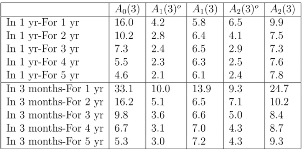
2(3)o A2(3) In 1 yr-For 1 yr 66.1 14.2 24.9 21.3 57.1 In 1 yr-For 2 yr 51.7 10.9 28.3 14.3 33.7 In 1 yr-For 3 yr 40.9 10.2 29.6 10.3 25.3 In 1 yr-For 4 yr 32.4 9.9 29.7 8.8 24.5 In 1 yr-For 5 yr 26.3 9.5 29.5 8.6 25.5 In 3 months-For 1 yr 95.1 24.0 29.7 35.4 108.5 In 3 months-For 2 yr 62.1 16.6 29.9 25.3 53.9 In 3 months-For 3 yr 48.6 13.3 32.1 18.1 32.6 In 3 months-For 4 yr 37.8 11.9 33.0 14.5 25.2 In 3 months-For 5 yr 30.1 11.5 33.0 13.0 24.7
Table 5: Relative Pricing Errors in % for At-the-Money Swaption
A0(3) A1(3)o A1(3) A
2(3)o A2(3) In 1 yr-For 1 yr 16.0 4.2 5.8 6.5 9.9 In 1 yr-For 2 yr 10.2 2.8 6.4 4.1 7.5 In 1 yr-For 3 yr 7.3 2.4 6.5 2.9 7.3 In 1 yr-For 4 yr 5.5 2.3 6.3 2.5 7.6 In 1 yr-For 5 yr 4.6 2.1 6.1 2.4 7.8 In 3 months-For 1 yr 33.1 10.0 13.9 9.3 24.7 In 3 months-For 2 yr 16.2 5.1 6.5 7.1 10.2 In 3 months-For 3 yr 9.8 3.6 6.6 5.0 8.4 In 3 months-For 4 yr 6.7 3.1 7.0 4.3 8.7 In 3 months-For 5 yr 5.3 3.0 7.2 4.3 9.3
Table 6: At-the-Money Swaption Implied Volatility Errors
A0(3) A1(3)o A1(3) A
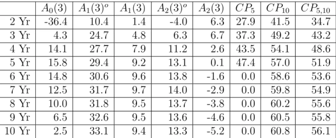
2(3)o A2(3) CP5 CP10 CP5,10 2 Yr -36.4 10.4 1.4 -4.0 6.3 27.9 41.5 34.7
3 Yr 4.3 24.7 4.8 6.3 6.7 37.3 49.2 43.2
4 Yr 14.1 27.7 7.9 11.2 2.6 43.5 54.1 48.6 5 Yr 15.8 29.4 9.2 13.1 0.1 47.4 57.0 51.9 6 Yr 14.8 30.6 9.6 13.8 -1.6 0.0 58.6 53.6 7 Yr 12.5 31.7 9.7 14.0 -2.9 0.0 59.8 54.9 8 Yr 10.0 31.8 9.5 13.7 -3.8 0.0 60.2 55.6 9 Yr 6.5 32.6 9.5 13.6 -4.6 0.0 60.5 55.8 10 Yr 2.5 33.1 9.4 13.3 -5.2 0.0 60.8 56.1
Table 7: In-Sample Predictability of Excess Returns (R2’s in %) This Table presents R2s obtained from projections of weekly realized zero coupon returns, for different maturities, on model in-sample implied returns.
CP5 is the prediction from a regression of excess returns on 1-year zero rates and 1-year forward rates at 1-, 2-, 3-, and 4-years. CP10 is the prediction from a regression of excess returns on 1-year zero rates and 1-year forward rates at 1-, 2-, 3-, 4-, 5-, 6-, 7-, 8-, 9-, and 10-years. CP5,10 use only 5 forward rates as regressors ranging up to 10 years. Regressions are based on overlapping data. The A0(3), A1(3), and A2(3) models were estimated by inverting 3-month, 2-year, and 10-year swap zeros and measuring 1-, 3-, 5-, and 7-year zeros with error. The A1(3)o and A2(3)o models were estimated with the additional
Jan96 Jan97 Jan98 Jan99 Jan00 Jan01 Jan02 Jan03 Jan04 0
0.002 0.004 0.006 0.008 0.01 0.012 0.014 0.016 0.018 0.02
2 Year cap price
data A
0(3) A
1(3) o A
1(3) A
2(3) o A
2(3)
Jan96 Jan97 Jan98 Jan99 Jan00 Jan01 Jan02 Jan03 Jan04 0
0.01 0.02 0.03 0.04 0.05 0.06
5 Year cap price
data A0(3) A1(3)o A1(3) A2(3)o A2(3)
Figure 1: Cap Prices
The top figure plots 2-year at-the-money cap prices. The bottom figure plots 5-year at-the-money cap prices. The actual prices are plotted with a solid black line. The prices from the A0(3) model plotted with a solid pink line. The prices from the A1(3) model are plotted with a solid blue line and the prices from theA1(3)omodel are plotted with a solid red line. The prices from
the A2(3) model are plotted with a dashed blue line and the prices from the
A2(3)o model are plotted with a dashed red line. TheA0(3), A1(3), andA2(3)
Jan96 Jan97 Jan98 Jan99 Jan00 Jan01 Jan02 Jan03 Jan04 1 2 3 4 5 6 7x 10
−3
price
In 3 months−For 2 yr model ATM swaption
data A0(3) A1(3)o
A1(3) A2(3)o
A2(3)
Jan96 Jan97 Jan98 Jan99 Jan00 Jan01 Jan02 Jan03 Jan04 0 0.2 0.4 0.6 0.8 1 1.2 1.4 Implied Volatility
In 3 months−For 2 yr model ATM swaption
data A0(3)
A1(3) o
A1(3)
A2(3) o
A2(3)
Jan96 Jan97 Jan98 Jan99 Jan00 Jan01 Jan02 Jan03 Jan04 2 4 6 8 10 12 14 16x 10
−3
price
In 3 months−For 5 yr model ATM swaption
data A0(3)
A1(3)o
A1(3) A2(3)o
A2(3)
Jan96 Jan97 Jan98 Jan99 Jan00 Jan01 Jan02 Jan03 Jan04 0.05 0.1 0.15 0.2 0.25 0.3 0.35 0.4 0.45 0.5 0.55 Implied Volatility
In 3 months−For 5 yr model ATM swaption
data A0(3)
A1(3) o
A1(3)
A2(3) o
A2(3)
Figure 2: In 3 Months At-the-Money Swaption Implied Volatilities
These figures plot prices and Black’s implied volatilities for at-the-money in-3-months-for-2-year and in-3-months-for-5-year swaptions. The at-the-money strike rates are the forward swap rates which are taken from the model. The data are plotted with a solid black line. The values from the A0(3) model plotted with a solid pink line. The values from the A1(3) model are plotted with a solid blue line and the values from the A1(3)o model are plotted with
a solid red line. The values from the A2(3) model are plotted with a dashed blue line and the values from the A2(3)o model are plotted with a dashed
Jan96 Jan97 Jan98 Jan99 Jan00 Jan01 Jan02 Jan03 Jan04 2 4 6 8 10 12 14x 10
−3
price
In 1 yr−For 2 yr model ATM swaption
data A0(3)
A1(3)o
A1(3) A2(3)o
A2(3)
Jan96 Jan97 Jan98 Jan99 Jan00 Jan01 Jan02 Jan03 Jan04 0 0.1 0.2 0.3 0.4 0.5 0.6 0.7 0.8 Implied Volatility
In 1 yr−For 2 yr model ATM swaption
data A0(3)
A1(3) o
A1(3)
A2(3) o
A2(3)
Jan96 Jan97 Jan98 Jan99 Jan00 Jan01 Jan02 Jan03 Jan04 0.005 0.01 0.015 0.02 0.025 0.03 price
In 1 yr−For 5 yr model ATM swaption
data A 0(3) A 1(3) o
A1(3)
A2(3) o
A2(3)
Jan96 Jan97 Jan98 Jan99 Jan00 Jan01 Jan02 Jan03 Jan04 0.05 0.1 0.15 0.2 0.25 0.3 0.35 0.4 0.45 Implied Volatility
In 1 yr−For 5 yr model ATM swaption
data A0(3)
A1(3) o
A1(3)
A2(3) o
A2(3)
Figure 3: In 1 Year At-the-Money Swaption Implied Volatilities
These figures plot prices and Black’s implied volatilities for at-the-money in-1-year-for-2-year and in-1-year-for-5-year swaptions. The at-the-money strike rates are the forward swap rates which are taken from the model. The data are plotted with a solid black line. The values from the A0(3) model plotted with a solid pink line. The values from the A1(3) model are plotted with a solid blue line and the values from the A1(3)o model are plotted with a solid red line. The values from theA2(3) model are plotted with a dashed blue line and the values from the A2(3)o model are plotted with a dashed red line. The
A0(3), A1(3), andA2(3) models were estimated by inverting 3-month, 2-year, and 10-year swap zeros and measuring 1-, 3-, 5-, and 7-year zeros with error. The A1(3)o and A2(3)o models were estimated with the additional assumption
Jan96 Jan97 Jan98 Jan99 Jan00 Jan01 Jan02 Jan03 Jan04 0 0.5 1 1.5 2 2.5x 10
−3
0.5 year volatility
EGARCH(1,1) Rolling Window EWMA A1(3)
o
A1(3)
Jan96 Jan97 Jan98 Jan99 Jan00 Jan01 Jan02 Jan03 Jan04 0 0.5 1 1.5 2 2.5 3 3.5x 10
−3
0.5 year volatility
EGARCH(1,1) Rolling Window EWMA A2(3)
o
A2(3)
A0(3)
Jan96 Jan97 Jan98 Jan99 Jan00 Jan01 Jan02 Jan03 Jan04 0.6 0.8 1 1.2 1.4 1.6 1.8 2 2.2 2.4x 10
−3
2 year volatility
EGARCH(1,1) Rolling Window EWMA A1(3)
o
A1(3)
Jan96 Jan97 Jan98 Jan99 Jan00 Jan01 Jan02 Jan03 Jan04 0.6 0.8 1 1.2 1.4 1.6 1.8 2 2.2 2.4 2.6x 10
−3
2 year volatility
EGARCH(1,1) Rolling Window EWMA A2(3)
o
A2(3)
A0(3)
Jan96 Jan97 Jan98 Jan99 Jan00 Jan01 Jan02 Jan03 Jan04 0.6 0.8 1 1.2 1.4 1.6 1.8 2 2.2x 10
−3
5 year volatility
EGARCH(1,1) Rolling Window EWMA A1(3)
o
A1(3)
Jan96 Jan97 Jan98 Jan99 Jan00 Jan01 Jan02 Jan03 Jan04 0.6 0.8 1 1.2 1.4 1.6 1.8 2 2.2x 10
−3
5 year volatility
EGARCH(1,1) Rolling Window EWMA A2(3)
o
A2(3)
A0(3)
Figure 4: Realized Volatility
These figures plot model conditional volatility of zero coupon rates against various estimates of conditional volatility using historical data. For estimates of conditional volatility based on historical data we use a 26 week rolling window, an exponential weighted moving average (EWMA) with a 26-week half-life, and estimate an EGARCH(1,1) for each maturity. The A0(3), A1(3), and A2(3) models were estimated by inverting 3-month, 2-year, and 10-year swap zeros and measuring 1-, 3-, 5-, and 7-year zeros with error. The A1(3)o
A0(3) A1(3)o A1(3) A
2(3)o A2(3) CP5 CP10 CP5,10 2 Yr -50.7 10.1 5.6 -2.3 9.8 22.2 -95.6 21.5 3 Yr -40.5 22.7 6.7 5.2 8.1 27.1 -85.9 24.8 4 Yr -39.2 24.1 10.7 11.7 2.8 31.8 -76.2 28.2 5 Yr -40.8 25.9 13.8 16.7 -0.5 36.1 -66.6 31.7 6 Yr -38.8 25.0 14.8 19.7 -3.0 0.0 -64.0 34.9 7 Yr -37.7 28.5 15.7 22.7 -4.7 0.0 -64.0 33.8 8 Yr -40.9 32.8 16.1 24.2 -5.2 0.0 -65.4 30.0 9 Yr -42.7 34.1 15.8 25.1 -5.9 0.0 -68.9 27.9 10 Yr -44.0 35.4 15.3 25.3 -6.4 0.0 -71.4 24.8
Table 8: Out-of-Sample Predictability of Excess Returns (R2’s in %) This Table presents R2s obtained from projections of weekly realized zero coupon returns, for different maturities, on model out-of-sample implied re-turns. CP5 is the prediction from a regression of excess returns on 1-year zero rates and 1-year forward rates at 1-, 2-, 3-, and 4-years. CP10 is the prediction from a regression of excess returns on 1-year zero rates and 1-year forward rates at 1-, 2-, 3-, 4-, 5-, 6-, 7-, 8-, 9-, and 10-years. CP5,10 use only 5 forward rates as regressors ranging up to 10 years. Regressions are based on overlap-ping data. The A0(3), A1(3), and A2(3) models were estimated by inverting 3-month, 2-year, and 10-year swap zeros and measuring 1-, 3-, 5-, and 7-year zeros with error. The A1(3)o and A2(3)o models were estimated with the
A0(3) A1(3)o A1(3) A2(3)o A2(3) CP5
2 Year 48 25 10 17 18 37
3 Year 79 46 17 30 23 80
4 Year 107 69 23 42 24 119
5 Year 136 92 27 51 24 158
6 Year 165 114 30 58 23
7 Year 195 134 32 64 22
8 Year 224 153 34 68 21
9 Year 253 170 36 72 21
10 Year 282 185 38 76 21
Table 9: Time Variation in Expected Returns.
This table contains the 1-week variance of 1-year expected excess return (ex-pressed in basis points). The A0(3), A1(3), and A2(3) models were estimated by inverting 3-month, 2-year, and 10-year swap zeros and measuring 1-, 3-, 5-, and 7-year zeros with error. The A1(3)o and A2(3)o models were estimated with the additional assumption that 1-, 2-, 3-, 4-, 5-, 7-, and 10-year at-the-money caps were measured with error. CP5 is the prediction from a regression of excess returns on 1-year zero rates and 1-year forward rates at 1-, 2-, 3-, and 4-years.
A0(3) A1(3)o A1(3) A2(3)o A2(3) First Eigenvalue 1.18 1.53 2.29 1.62 1.81 Second Eigenvalue 0.34 0.57 0.17 0.17 0.64 Third Eigenvalue 0.03 0.57 0.00 0.13 0.04
Table 10: Eigenvalues ofKP
1 Matrix
A0(3) A1(3)o A1(3) A2(3)o A
2(3) First Eigenvalue 1.08 1.71 2.30 2.62 2.38 Second Eigenvalue 0.75 0.54 0.53 0.42 0.57 Third Eigenvalue 0.02 0.12 0.05 0.13 0.05
Jan96 Jan97 Jan98 Jan99 Jan00 Jan01 Jan02 Jan03 −0.1
−0.05 0 0.05 0.1 0.15
Excess returns
realized return $A
0(3)$
$A
1(3) o$
$A1(3)$ $A2(3)o$ $A2(3)$ CP − 5 Yr
Figure 5: Excess Returns
This figure plots weekly realized excess returns, and model implied expected excess returns for a 5 year zero coupon bond. Realized excess returns are plotted with a solid black line. Predicted excess returns from the A0(3) model are plotted with a solid pink line. Predicted excess returns from the A1(3) model are plotted with a solid blue line and those from the A1(3)o model are
plotted with a solid red line. Predicted excess returns from theA2(3) model are plotted with a dashed blue line and those from the A2(3)o model are plotted