Consumption-Wealth Ratio and Expected
Stock Returns: Evidence from Panel Data
on G7 Countries
*
Andressa Monteiro de Castro
†
João Victor Issler
‡
Contents: 1. Introduction; 2. Present-Value Theory; 3. Macroeconomic and Financial Data; 4. Cointegration Analysis (cay); 5. Forecasting Stock Returns In-Sample; 6. Out-of-Sample Forecasts; 7. Cointegration and Forecasting with a FMOLS Estimate ofcay; 8. Conclusions; Appendix A. VECM Heterogeneous Cointegrating Vectors; Appendix B. FMOLS Heterogeneous Cointegrating Vectors.
Keywords: Consumption-Wealth Ratio, Stock Returns, Unbalanced Panel, Cointegrating Residual. JEL Code: C22, D91, E21.
Using the theoretical framework of Lettau & Ludvigson (2001), we perform an empirical investigation on how widespread is the predictability ofcay—a mod-ified consumption-wealth ratio—once we consider a set of important countries from a global perspective. We chose to work with the set of G7 countries, which represent more than 64% of net global wealth and 46% of global GDP at market exchange rates. We evaluate the forecasting performance ofcayusing a panel-data approach, since applying cointegration and other time-series techniques is now standard practice in the panel-data literature. Hence, we generalize Lettau and Ludvigson’s tests for a panel of important countries. We employ macroe-conomic and financial quarterly data for the group of G7 countries, forming an unbalanced panel. For most countries, data is available from the early 1990s until 2014Q1, but for the U.S. economy it is available from 1981Q1 through 2014Q1. Results of an exhaustive empirical investigation are overwhelmingly in favor of the predictive power ofcayin forecasting future stock returns and excess returns.
Usando o arcabouço teórico de Lettau & Ludvigson (2001), investigamos a existência de previsibilidade vis-à-vis os excessos de retorno de uma versão modificada da razão
*We are especially grateful for the comments and suggestions given by Wagner Gaglianone, Pedro Cavalcanti Ferreira, Ricardo
Sousa and other seminar participants at the2nd International Workshop on “Financial Markets and Nonlinear Dynamics”(FMND) in Paris. Any remaining errors are ours. Both Castro and Issler gratefully acknowledge the support from CNPq, FAPERJ, INCT and FGV on different grants. We also thank Marcia Waleria Machado, Marcia Marcos, Andrea Virginia, and Rafael Burjack for excellent research assitence.
†Fundação Getúlio Vargas, Escola Brasileira de Economia e Finanças (FGV/EPGE). Praia de Botafogo 190, Rio de Janeiro, RJ, Brasil.
CEP 22250-900. Email:[email protected]
consumo-riqueza para os países do grupo G7. Num exercício empírico exaustivo, confirmamos a potencial previsibilidade da razão consumo-riqueza num arcabouço de dados de painel, algo inédito para esse representativo grupo de paises.
1. INTRODUCTION
The link between macroeconomic and financial markets has long driven a great deal of theoretical and empirical work in the macroeconometric literature. Taking the asset-pricing equation as a starting point, and using a present-value approach, one can derive several interesting implications between macroe-conomic data and future returns or excess returns. The work of Campbell (1987), Campbell & Shiller (1987, 1988a), Campbell & Deaton (1989), and Campbell & Mankiw (1989), are good early examples of the connection between macroeconomic and financial variables. Indeed, one should expect some asset-return predictability following this literature, although the evidence is weak. Compare, for example, the results in Fama & French (1988) and Pesaran & Timmermann (1995) with those in Campbell & Thompson (2008). Recently, Guillén, Issler, & Saraiva (2015) examine the usefulness of imposing different layers of present-value-model restrictions in forecasting financial data — a directly related issue.
In an interesting paper, Lettau & Ludvigson (2001) study the role of transitory trend deviations for consumption, asset holdings and labor income in predicting future stock market fluctuations. Using a forward-looking model, with a novel present-value equation, they show that, when investors expect higher returns in the future, they react by raising current consumption relative to its trend vis-a-vis asset wealth and labor income in order to smooth consumption in line with the asset-pricing equation. Therefore, these current transitory fluctuations of consumption about its trend carry information about the future dynamics of returns and excess returns. These issues are investigated using the time-series framework of cointegration and cross-equation restrictions in the context of a vector autoregressive (VAR) model.
Despite the strong empirical evidence provided by Lettau & Ludvigson (2001) for the U.S. stock market, there has been only a few papers trying to investigate this issue with an a broader interna-tional perspective. For example, Ioannidis, Peel, & Matthews (2006), Tsuji (2009) and Gao & Huang (2008) extended the time-series analysis of Lettau & Ludvigson (2001) to other countries, which yields country-specific results. Nitschka (2010), on the other hand, used the consumption-wealth ratio of the U.S. economy as a predictor of foreign stock returns. In a more elaborate paper, Sousa (2010) shows that housing wealth could be an important component of aggregate wealth when predicting asset returns.
Despite the unquestionable value-added of the subsequent literature, what we see as lacking in it is the use of a broad enough approach to test the idea that transitory trend deviations for consumption (c), asset-wealth holdings (a) and labor income (y) are able to predict future stock market fluctuations, i.e., the usefulness ofcay in forecasting returns. If the present-value model holds, it should hold for every country, and not only to the U.S. economy. Instead of employing a country-specific approach to the matter, we propose to use a panel-data approach for a group of relevant countries, which will be able to test the predictability theory in a broader sense. In order to cover a group of relevant countries, we decided to focus on the G7 group: Canada, France, Germany, Italy, Japan, the United Kingdom and the United States.
will be highly informative for global financial markets. Additional advantages of employing panel-data tests vis-a-vis country specific tests is the fact that one gathers more information using the former—the cross-sectional dimension.
The first step of our empirical analysis is to test for the existence of a single cointegrating re-lationship among consumption, asset wealth, and labor income, with panel cointegration tests. Our performed tests allow for heterogeneity in the linear combination forming the cointegrating relation-ship (cayh) as well as imposing homogeneity restrictions in it (cay). Here, we also discuss whether or not the estimated linear combinations (cayL and cayLh) conform to theory in some respects, looking at alternative estimates in the cases where they do not. With our estimates in hand, the next step is to implement an in-sample forecasting exercise, where we investigate whether or notcayL andcayLh help to forecast future stock returns and excess returns. We also include in these regressions some financial variables that are widely used in the literature to predict stock returns. Our final forecasting test asks whether or notcayL and cayLh help to forecast future stock returns out of sample. Here, the forecast-ing regression is recursively re-estimated, mimickforecast-ing closely the exercise a financial analyst will do in practice. Again, we employ a variety of alternative predictors in a horse-race between cayL (orcayLh) and these potential predictors. Finally, we repeat the in-sample and out-of-sample forecasting tests for cointegrating results that did not conform to theory.
In performing our empirical tests we employ macroeconomic real quarterly data per capita, mea-sured in 2010 country’s own currency, as well as financial data for returns and excess returns. Our main sources of data are the National Accounts Statistics of the OECD database, the Federal Reserve Economic Data (FRED) of the FED of St. Louis, and the International Financial Statistics (IFS), provided by the IMF. We have an unbalanced panel. For most countries, data is available from the early 1990s until 2014Q1, but for the U.S. economy it is available from 1981Q1 through 2014Q1.
Our final results allow for a very broad examination of the present-value theory behindcay, and its potential forecasting power for future returns. First, we find overwhelming evidence of a single cointegration vector for consumption, asset wealth, and labor income. This is true whether or not we allow for heterogeneity in computing the cointegrating relationship. Despite these results, in some cases the coefficients in the linear combination did not conform to theory. The coefficients of asset wealth and labor income must reflect the participation of asset wealth and human capital in total wealth. Thus, they must lie between zero and one and add up to unity. These theoretical restrictions did not hold in some cases, which required alternative estimation techniques. Second,cayL andcayLh help to forecast future stock returns and excess returns in sample. This is true whether or not we consider additional regressors in forecasting. Third,cayL andcayLhhelp to forecast future stock returns and excess returns in the out-of-sample exercise, usually performing better than alternative regressors. Finally, using estimates of cay andcayhthat conform to economic theory does improve forecasts of future accumulated excess returns.
The next section presents a brief review of the theoretical framework which establishes the present-value relationship betweencayand expected stock returns. In section 2, we thoroughly detail the ag-gregate and financial data that we use to construct our panel. Section 3 presents the results of the integration and cointegration analyses in a penal-data context, i.e., we build the estimates of cayand cayh. Section 4 reports the results of in-sample forecasting. In section 5, we perform out-of-sample forecasts. In section 6, we re-estimate cay and cayh using the fully-modified OLS (FMOLS) estimator to obtain cointegration estimates that conform to theory. Then, we revisit our previous forecasting exercise. Finally, in section 7, we conclude.
2. PRESENT-VALUE THEORY
the net return on aggregate invested wealth. The budget constraint faced by this agent is
Wt+1=(1+Rw,t+1 ) (W
t−Ct). (1)
Campbell & Mankiw (1989) suggest log-linearizing (1), obtaining
∆wt+1≈rw,t+1+ (
1−1/ρw) (ct−wt)+k1, (2)
where the lower case letters from now on are used to denote the logs of the corresponding variables, rw,t+1
≡log(1+R);ρwis the steady-state proportion of investment on wealth; andk1is a non-interesting
constant. For future reference, allki,i=2,3,. . ., are constants as well.
If the consumption-wealth ratio is stationary, it is possible to solve this equation forward in ex-pectations. Thus, taking the conditional expectation and assuming that the transversality condition
limi→∞Et
[
ρiw(ct+i−wt+i)
]
=0holds, the log consumption-wealth may be written as
ct−wt=Et
∞
∑
i=1 ρiw(
rw,t+i
−∆ct+i)+k2, (3)
which means that there is a present value relationship between consumption-wealth ratio and the return on aggregate wealth.
A main problem with (3) is that total wealth has two components: asset wealth and human capital. However, the latter is non observable. Lettau & Ludvigson (2001) deal with this issue in an elegant way. They define aggregate wealth as asset wealth plus human capitalWt =At+Ht, the log of aggregate wealth may be approximated as
wt ≈γ at+(1−γ)ht+k3, (4)
whereγ is the average share of asset holdings in total wealth. Furthermore, Campbell (1996) shows that the return to aggregate wealth, which is given by
1+Rw,t =γt (1
+Ra,t )
+(1−γt) (1
+Rh,t
), (5)
may be log-linearized to get to a tractable intertemporal model with constant coefficients:
rw,t
≈γ ra
,t+(1
−γ)rh
,t+k4. (6)
Substituting (4) and (6) into (3), gives
ct−γ at−(1−γ)ht=Et ∞
∑
i=1 ρwi
[
γ ra,t+i+(1−γ)rh,t+i
−∆ct+i]+k5. (7)
To deal with non observable that human capital, Lettau & Ludvigson (2001) use the fact that labor income can be interpreted as the dividend on human wealth, implying
(
1+Rh,t+1 )
=Ht+1+Yt+1 Ht
. (8)
Once more, log-linearizing this expression, we obtain:
rh,t+1
≈ρhht+1+(1−ρh)yt+1−ht+k6,
where ρh is the steady-state proportionH/(H+Y). Solving it forward, taking the expectation and imposing thatlimi→∞Et
[ ρih(
ht+i−yt+i)
]
=0, the log human capital can be described as
ht=yt+Et
∞
∑
i=1 ρih(
∆yt+i−rh,t+i )
Lettau & Ludvigson (2001) show that the nonstationary component of human capital is captured by labor income, implying thatht =κ+yt+µt, whereκis a constant. It is easy to see from (9) that µt=Et∑∞
i=1ρih
(∆y
t+i−rh,t+i
). This term is a stationary random variable, since we are assuming that
∆yt is stationary—labor income has a unit root—and that the return on human wealth is practically constant.
Replacing the log of human wealth in expression (7) by the one obtained in (9), it is possible to rewrite the log consumption-wealth ratio in terms of observable variables:
cayt≡ct−γ at−(1−γ)yt (10)
=Et
∞
∑
i=1 ρwi
[
γ ra,t+i+(1−γ)rh,t+i−∆ct+i ]
+(1−γ)µt+k8. (11)
Under the assumption thatrw,t,∆ct and ∆yt are stationary,
1equations (10) and (11) imply that ct,at andyt are cointegrated andct−γ at−(1−γ)yt is the cointegrating linear combination labelled ascayt, where (1,−γ,−(1−γ)) is the cointegrating vector (Lettau & Ludvigson, 2004). Besides,cay
t Granger-causes the right-hand term in brackets, since these terms are dated fromt+1onwards. There-fore, provided that the expected future returns on human capital and consumption growth are relatively smooth, changes incayt should forecast future changes on asset returns.2
This result is by and large consistent with a wide range of forward-looking models of investor behavior, where agents, disliking sharp fluctuations on consumption, will attempt to smooth out transi-tory movements in asset wealth due to variations in future expected asset returns. For instance, when higher returns are expected in the future, the forward-looking investors will currently increase their consumption out of their asset wealth and labor income, rising consumption above trend—an increase incayt—and vice-versa for the case when lower returns are expected in the future.
3. MACROECONOMIC AND FINANCIAL DATA
We work with a typical panel of macroeconomic data, where the cross-sectional dimension is small and the time-series dimension is large. As noted above, we possess an unbalanced panel for G7 countries:3: Canada, France, Germany, Italy, Japan, United Kingdom and United States. All aggregate variables are quarterly, seasonally adjusted, per capita, and measured in 2010 country’s own currency. To deflate data we use the CPI from International Financial Statistics (IFS)—the IMF database—and for quarterly population figures we interpolate annual data provided by OECD.
Consumption data used here is private final consumption expenditure from National Accounts Statistics of OECD’s database. Labor income used here is the compensation of employees, provided by the Federal Reserve Economic Data (FRED) of the Federal Reserve Bank of St. Louis, but the original source is OECD as well. Asset holdings data were taken separately from each of the G7 country’s central bank. Asset holdings is a critical variable in our analysis, since it determines the time span for each country in the database. Tabela 1 specifies the details of thefinancial asset holdingsdata used in this paper.
Real asset returns and excess returns are obtained from stock indices. To obtain the log of real gross returnsrtfor each country, we take their quarterly closing prices, adjusted for dividends. Nominal
1We test the evidence of unit root process in consumption and labor income in our panel data. Both don’t reject at 5% significance
level the null hypothesis of unit root, including individual effects and individual linear trends.
2Lettau & Ludvigson (2001) find thatcay
t is a strong predictor of excess returns on aggregate US stock market indexes for both short and long run.
3The reason for choosing G7 is the lack of data availability for other countries in quarterly frequency, specially of households asset
Table 1.Data sources.
Canada
(1990Q1–2014Q1)
CANSIM, Statistics Canada: Net worth of households and non-profit institutions serving households (NPISH)
France
(1996Q1–2014Q1)
Webstat, Banque de France: Net financial assets of households and NPISH
Germany
(1991Q1–2014Q1)
Deutsche Bundesbank: Financial Asset of households and NPISH
Italy
(1995Q1–2014Q1)
BDS, Banca D’Italia: Total financial instruments held by households and NPISH
Japan
(1997Q4–2014Q1)
Bank of Japan: Total assets of households
United Kingdom
(1997Q1–2014Q1)
Bank of England: Financial assets of households and NPISH
United States
(1981Q1–2014Q1)
Board of Governors of the Federal Reserve System: Net worth of households and NPISH
stock indices are provided by Bloomberg and are deflated using the seasonally adjusted CPI figures from IFS. The stock indices used here are: S&P/TSX composite index for Canada, CAC 40 for France, DAX for Germany, FTSEMIB for Italy, Nikkei 225 for Japan, FTSE 100 for United Kingdom and S&P 500 for United States. To obtain quarterly log of excess returnsrt−rf,t, we need to specify the risk-free raterf,t. The
raw data is the percent per annum treasury bill rate from government securities for each country, taken from IFS.
We also considered some additional financial variables such as dividend yield, payout ratio and relative bill rate, in order to extend our analysis and compare the predictive power of cayand that of these variables. Here, we letd−p denote the dividend yield, whered is the log of quarterly dividends
per share andp is the log of the stock index. Since Campbell & Shiller (1988b), this variable has been widely used to forecast excess returns,4 especially for long horizons. Following Lamont (1998), the payout ratio is represented byd−e, whereeis the log of quarterly earnings per share. As well as the
stock index, both dividends per share and earnings per share are provided by Bloomberg. Finally, we build the relative bill rateRRELsubtracting from the T-bill rate its 12-month backward moving average, a method suggested by Hodrick (1992).
4. COINTEGRATION ANALYSIS (
cay
)
First, we test whether each of the variables incayt≡ct−γ at−(1−γ)yt—consumption (ct), asset wealth
(at), and labor income (yt)—have or not a unit root in (log) levels. We perform a panel unit root test proposed by Maddala & Wu (1999), which consists of a Fisher (1932) test5that combine the significance levels from individual unit root tests, such as Phillips–Perron (PP) and Augmented Dickey–Fuller (ADF).
4Campbell & Shiller (1988b) show that the log dividend-price ratio may be written asd
t−pt =Et∑∞
j=1ρ j
a(ra,t+j−∆dt+j
), which means that if the dividend-price ratio is high, agents must be expecting either high future asset returns or low dividend growth rates.
5We choose the Fisher test due to the structure of our data. The asymptotic validity for this test depend onT going to infinity,
For all three variables, in both tests—PP and ADF—the null hypothesis of presence of unit root is not rejected at a ten percent significance level,6which we interpret to mean that their process is integrated of order one.
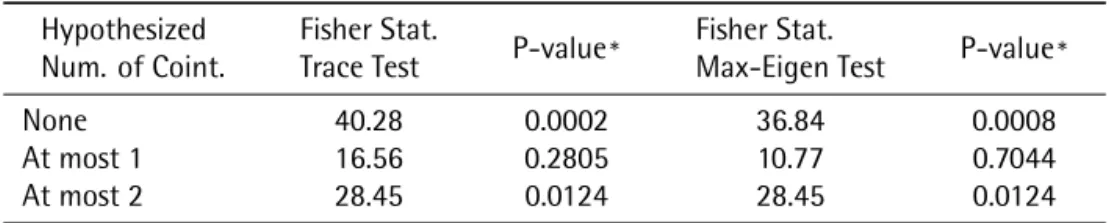
Next we conduct two panel cointegration tests to verify if there is a single cointegrating relation-ship among consumption, asset wealth and labor income. The first one is a residual-based test proposed by (Kao, 1999), in which homogeneity restrictions are imposed in the cointegrating vector. We strongly reject the null of no cointegration, with a p-value of 0.29%.7 This allows the conclusion of the existence of at least one cointegrating vector. The second test is another Fisher-type test suggested by Maddala & Wu (1999) using a Johansen (1991) procedure to determine the number of cointegrating relations among those three variables in the panel. Since the variables are integrated of order one, we can have zero, one, or two cointegrating vectors. In this case, no homogeneity restrictions are imposed for the cointegrating coefficients. Results are presented in Tabela 2, and indicate that there is indeed a single cointegrating vector for consumption, asset wealth and labor income. Therefore, we are confident that there is a sin-gle cointegrating vector for consumption, asset wealth, and labor income, these three variables sharing two common trends.
The next step is to estimate the parameters of the cointegrating vector,cayt≡ct−γ at−(1−γ)yt.
Instead of imposing a prioritheoretical restrictions, where 0 ≤γ ≤1, we estimate the coefficients
unrestricted, once imposing homogeneity restrictions—all coefficients are the same across the panel, and once without homogeneity restrictions—coefficients vary across cross-sectional units. In the former case, we estimate the following cointegrating vector:
cayt =ci,t
−βaai
,t
−βyyi
,t, (12)
whereas in the latter case, we estimate
cayhi,t =ci,t−βa,iai,t−βy,iyi,t. (13)
We estimate cointegrating vectors using Johansen (1991) full-information maximum likelihood (FIML) procedure. Regarding deterministic terms, we assume a linear deterministic trend in data. We chose a vector autoregressive (VAR) model of order two in levels. Tabela 3 presents the estimates of the cointe-grating parameters for (12).8 One can immediately see that the coefficient of labor income is negative, −0.6406, although it is not significant. Further unit root tests on the cointegrating residual confirm thatcayMt does not have a unit root.9
We now turn to the estimation of equation (13)—cointegrating vector without imposing homo-geneity restrictions. We estimate separately a vector error-correction model (VECM) for each country, with results reported in the Appendix A. Again, further unit root tests on the cointegrating residuals confirms thatcayLhi,t
does not have a unit root.
6Probabilities for Fisher test are computed using asymptoticχ2distribution.
7Probabilities for Kao test are computed using asymptotic Normal distribution
8With one lag in difference, linear trend and one cointegrating relationship, we estimate the following VEC through a pooled OLS.
∆ci,t=α1
(c
i,t−1−βaai,t−1−βyyi,t−1−µ
)
+γ11∆ci,t−1+γ12∆ai,t−1+γ13∆yi,t−1+η1+ϵ1,i,t
∆ai,t=α2
(
ci,t−1−βaai,t−1−βyyi,t−1−µ
)
+γ21∆ci,t−1+γ22∆ai,t−1+γ23∆yi,t−1+η2+ϵ2,i,t
∆yi,t=α3
(c
i,t−1−βaai,t−1−βyyi,t−1−µ
)
+γ31∆ci,t−1+γ32∆ai,t−1+γ33∆yi,t−1+η3+ϵ3,i,t.
The right-hand side variable in parenthesis is the error correction term. In long run equilibrium, this term should be zero. However, if any variable of this term deviates from the long run equilibrium, the error correction term would be nonzero and the other variables would adjust to restore the equilibrium relation. The coefficientsαmeasure the speed of adjustment of each endogenous variable towards the equilibrium (Engle & Granger, 1987).
Table 2.Johansen Fisher Panel Cointegrating Test.
Hypothesized Num. of Coint.
Fisher Stat.
Trace Test P-value*
Fisher Stat.
Max-Eigen Test P-value*
None 40.28 0.0002 36.84 0.0008
At most 1 16.56 0.2805 10.77 0.7044
At most 2 28.45 0.0124 28.45 0.0124
Notes:This table reports the panel cointegration test on consumption, asset wealth and income, assuming that there is a linear deterministic trend in data, including an intercept in the cointegration equation, and using one lag in difference (two lags in level) on the VAR tested.
*Probabilities are computed using asymptoticχ2distribution.
Table 3.Panel cointegrating vector estimates.
Estimated Parameters Asset Wealth Labor Income Constant
Consumption −1.4581*** 0.6406* 2.0963
(0.4292) (0.3674)
Notes:This table presents the estimated parameters of the cointegrating vector(1,−βDy,−βDa)from the VEC estimation, with respective standard errors in parenthesis. On the specification, we include an intercept in the cointegrating equation, once we assume there is a linear deterministic trend in data, we use one lag in difference and impose one cointegrating relationship. 594 observations are included in this estimation after adjustments. Statistics with * are significant at 10% level, **at 5% and***at 1%, computed using asymptotic Normal distribution.
One thing to note is that in the estimation of (12) and (13) we obtained some counter-intuitive results, or results that go against the present-value theory in section 2. These violations happen when
−βa’s or−βy’s are outside the interval[0,1], which happened for−βy in Tabela 3, and for−βa
,i and
−βy
,i for a few countries in Appendix A. It is hard to explain why these violations happen. There may
be measurement error on the data used; it can be the consequence of using a first-order approximation log linear approximation in building (11); etc. In any case, to deal with this issue, we will also consider alterative estimates of (12) and (13) in which these violations are much more infrequent; see the results in section 7.
5. FORECASTING STOCK RETURNS IN-SAMPLE
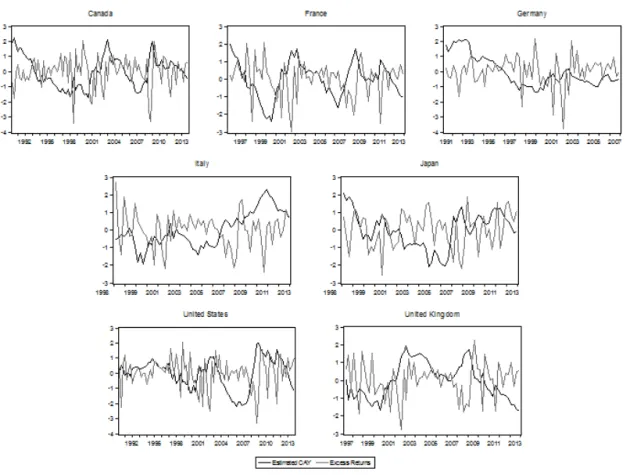
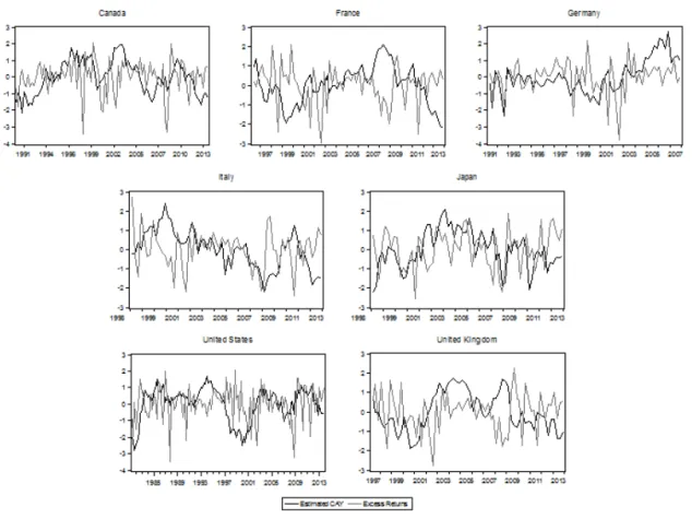
In this section, we investigate ifcaycan anticipate real stock returns and real excess returns in sample using a panel-data structure. The intuition here is that variations oncayshould precede variations on stock returns, since, theoretically, the forward-looking investor would increase or decrease current con-sumption with regard to his wealth, according to future fluctuations on expected stock returns. Figura 1 presents individual graphs for log excess returns—log returns on stock indexes minus the log return on T-bill—andcayL normalized series.10
For some countries such as Canada, France, Japan and United Kingdom, sharp variations ofcayL clearly preceding spikes in excess returns, for both positive and negative fluctuations. It is also inter-esting to note that recently most countries have presented a pronounced decreasing in cayL. Another feature ofcayL is its counter-cyclical behavior. In fact, when we make a panel regression of consumption
10Here, we disaggregate the panel into seven time series, one for each country, and detrend them individually in order to eliminate
Figure 1.Excess Returns and Estimatedcay.
growth on contemporaneouscayL controlling for cross section fixed effects, we obtain a coefficient of −0.005181 statistically significant at the 1% level.
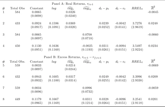
Tabela 4 presents in-sample one-quarter-ahead regressions with real returns and excess returns as dependent variables and both cayL and cayLh and other financial variables as regressors, including cross-section fixed effects. On all of these regressions, we make White cross-section corrections to the standard errors.11 Regressions with one-period lag of the dependent variable as a regressor are also computed on Tabela 4. It is well known that the LSDV (least squares dummy variable)—the “fixed effects model” we have used in the previous regressions—with a lagged dependent variable generates biased estimates when the time dimension of the panel is small (Judson & Owen, 1999). Nevertheless, Nickell (1981) derives an expression for the bias showing that it goes to zero whenT approaches infinity. For our purposes, since we are under a largeT, smallN, environment, the LSDV model bias should be very small, we thus take these in-sample results seriously. Again, we use the White cross-section correction in these regressions as well.
11This method considers the pool regression as multivariate regressions with one equation for each cross-section, and computes
for the system of equations robust standard errors. The robust variance matrix estimator is given by
Avar(βˆ)≡
(
NT NT−K
) ( ∑
t
X′
tXt )−1(
∑
t
X′
tϵˆtϵˆt′Xt ) (
∑
t
X′
tXt )−1
,
Table 4. In-sample one-quarter-ahead regressions.
Panel A: Real Returns,rt+1
# Total Obs Constant lag dcayt cay[ht dt pt dt et RRELt R
2
1 584 0.0065 0.0326 -0.0045
(0.0098) (0.0240)
2 433 0.0924 0.1596 0.0369 0.0239 -0.0042 3.7276 0.0248
(0.0917) (0.1091) (0.0320) (0.0252) (0.0141) (2.9619)
3 584 0.0065 0.0708 -0.0060
(0.0097) (0.0718)
4 450 0.1130 0.1636 -0.0025 0.0311 -0.0094 3.5497 0.0234
(0.0951) (0.1160) (0.1193) (0.0261) (0.0151) (2.9224)
Panel B: Excess Returns,rt+1 rf;t+1
# Total Obs. Constant lag dcayt cay[ht dt pt dt et RRELt R
2
5 559 0.0033 0.0214 -0.0069
(0.0097) (0.0244)
6 432 0.0943 0.1605 0.0317 0.0249 -0.0042 3.3996 0.0209
(0.0932) (0.1100) (0.0314) (0.0255) (0.0142) (2.9338)
7 559 0.0034 0.0996 -0.0059
(0.0096) (0.0732)
8 449 0.1179 0.1667 0.0311 0.0328 -0.0096 3.2541 0.0201
(0.0965) (0.1169) (0.1214) (0.0264) (0.0151) (2.9118)
Notes:This table shows some regressions of one-step-forward returns forecasts. Total Obs. refers to the total panel unbalanced observations included after adjustments, andlagis the one-lag backward dependent variable, i.e. ont, used as a regressor. The Constant is an overall fixed effects mean and we omit the specific fixed effects of each country. The last column reports the adjustedR2. White cross-section corrected standard errors appear in parenthesis.
In Tabela 4, at one-quarter ahead, bothcayL andcayMhare not able to predict stock returns, since
their coefficients are not statistically significant. The same is true for the other financial variables con-sidered in Tabela 4. It is also worth noting that theR2are extremely low, especially on the regressions with eithercayL orcayLh as a single regressor.
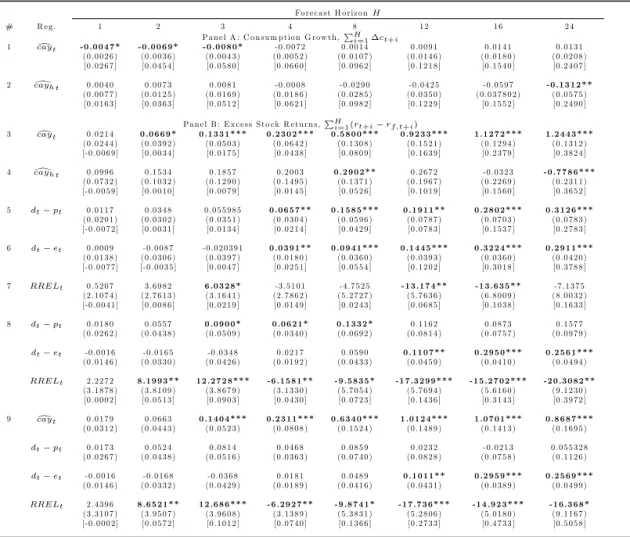
From equation (11), one can conclude thatcayshould be a good predictor of consumption growth as well as of asset returns. Thus, we investigate whether or not it helps to forecast either accumulated consumption growth or accumulated excess returns. Tabela 5 presents the results over horizons span-ning 1 to 24 quarters, where regressions are estimated by the LSDV model. Results are presented in Tabela 5.
Table 5. In-sample long-horizon regressions.
Fo re c a st H o riz o nH
# R e g . 1 2 3 4 8 1 2 1 6 2 4
P a n e l A : C o n su m p tio n G row th ,PH i=1 ct+i
1 caydt - 0 .0 0 4 7 * - 0 .0 0 6 9 * - 0 .0 0 8 0 * -0 .0 0 7 2 0 .0 0 1 4 0 .0 0 9 1 0 .0 1 4 1 0 .0 1 3 1
(0 .0 0 2 6 ) (0 .0 0 3 6 ) (0 .0 0 4 3 ) (0 .0 0 5 2 ) (0 .0 1 0 7 ) (0 .0 1 4 6 ) (0 .0 1 8 0 ) (0 .0 2 0 8 ) [0 .0 2 6 7 ] [0 .0 4 5 4 ] [0 .0 5 8 0 ] [0 .0 6 6 0 ] [0 .0 9 6 2 ] [0 .1 2 1 8 ] [0 .1 5 4 0 ] [0 .2 4 0 7 ]
2 cay[h t 0 .0 0 4 0 0 .0 0 7 3 0 .0 0 8 1 -0 .0 0 0 8 -0 .0 2 9 0 -0 .0 4 2 5 -0 .0 5 9 7 - 0 .1 3 1 2 * * (0 .0 0 7 7 ) (0 .0 1 2 5 ) (0 .0 1 6 9 ) (0 .0 1 8 6 ) (0 .0 2 8 5 ) (0 .0 3 5 0 ) (0 .0 3 7 8 0 2 ) (0 .0 5 7 5 ) [0 .0 1 6 3 ] [0 .0 3 6 3 ] [0 .0 5 1 2 ] [0 .0 6 2 1 ] [0 .0 9 8 2 ] [0 .1 2 2 9 ] [0 .1 5 5 2 ] [0 .2 4 9 0 ]
P a n e l B : E x c e ss S to ck R e tu rn s,PH
i=1(rt+i rf;t+i)
3 caydt 0 .0 2 1 4 0 .0 6 6 9 * 0 .1 3 3 1 * * * 0 .2 3 0 2 * * * 0 .5 8 0 0 * * * 0 .9 2 3 3 * * * 1 .1 2 7 2 * * * 1 .2 4 4 3 * * * (0 .0 2 4 4 ) (0 .0 3 9 2 ) (0 .0 5 0 3 ) (0 .0 6 4 2 ) (0 .1 3 0 8 ) (0 .1 5 2 1 ) (0 .1 2 9 4 ) (0 .1 3 1 2 ) [-0 .0 0 6 9 ] [0 .0 0 3 4 ] [0 .0 1 7 5 ] [0 .0 4 3 8 ] [0 .0 8 0 9 ] [0 .1 6 3 9 ] [0 .2 3 7 9 ] [0 .3 8 2 4 ]
4 cay[h t 0 .0 9 9 6 0 .1 5 3 4 0 .1 8 5 7 0 .2 0 0 3 0 .2 9 0 2 * * 0 .2 6 7 2 -0 .0 3 2 3 - 0 .7 7 8 6 * * * (0 .0 7 3 2 ) (0 .1 0 3 2 ) (0 .1 2 9 0 ) (0 .1 4 9 5 ) (0 .1 3 7 1 ) (0 .1 9 6 7 ) (0 .2 2 6 9 ) (0 .2 3 1 1 ) [-0 .0 0 5 9 ] [0 .0 0 1 0 ] [0 .0 0 7 9 ] [0 .0 1 4 5 ] [0 .0 5 2 6 ] [0 .1 0 1 9 ] [0 .1 5 6 0 ] [0 .3 6 5 2 ]
5 dt pt 0 .0 1 1 7 0 .0 3 4 8 0 .0 5 5 9 8 5 0 .0 6 5 7 * * 0 .1 5 8 5 * * * 0 .1 9 1 1 * * 0 .2 8 0 2 * * * 0 .3 1 2 6 * * * (0 .0 2 0 1 ) (0 .0 3 0 2 ) (0 .0 3 5 1 ) (0 .0 3 0 4 ) (0 .0 5 9 6 ) (0 .0 7 8 7 ) (0 .0 7 0 3 ) (0 .0 7 8 3 ) [-0 .0 0 7 2 ] [0 .0 0 3 1 ] [0 .0 1 3 4 ] [0 .0 2 1 4 ] [0 .0 4 2 9 ] [0 .0 7 8 3 ] [0 .1 5 3 7 ] [0 .2 7 8 3 ]
6 dt et 0 .0 0 0 9 -0 .0 0 8 7 -0 .0 2 0 3 9 1 0 .0 3 9 1 * * 0 .0 9 4 1 * * * 0 .1 4 4 5 * * * 0 .3 2 2 4 * * * 0 .2 9 1 1 * * * (0 .0 1 3 8 ) (0 .0 3 0 6 ) (0 .0 3 9 7 ) (0 .0 1 8 0 ) (0 .0 3 6 0 ) (0 .0 3 9 3 ) (0 .0 3 6 0 ) (0 .0 4 2 0 ) [-0 .0 0 7 7 ] [-0 .0 0 3 5 ] [0 .0 0 4 7 ] [0 .0 2 5 1 ] [0 .0 5 5 4 ] [0 .1 2 0 2 ] [0 .3 0 1 8 ] [0 .3 7 8 8 ]
7 RRELt 0 .5 2 0 7 3 .6 9 8 2 6 .0 3 2 8 * -3 .5 1 0 1 -4 .7 5 2 5 - 1 3 .1 7 4 * * - 1 3 .6 3 5 * * -7 .1 3 7 5 (2 .1 0 7 4 ) (2 .7 6 1 3 ) (3 .1 6 4 1 ) (2 .7 8 6 2 ) (5 .2 7 2 7 ) (5 .7 6 3 6 ) (6 .8 0 0 9 ) (8 .0 0 3 2 ) [-0 .0 0 4 1 ] [0 .0 0 8 6 ] [0 .0 2 1 9 ] [0 .0 1 4 9 ] [0 .0 2 4 3 ] [0 .0 6 8 5 ] [0 .1 0 3 8 ] [0 .1 6 3 3 ]
8 dt pt 0 .0 1 8 0 0 .0 5 5 7 0 .0 9 0 0 * 0 .0 6 2 1 * 0 .1 3 3 2 * 0 .1 1 6 2 0 .0 8 7 3 0 .1 5 7 7 (0 .0 2 6 2 ) (0 .0 4 3 8 ) (0 .0 5 0 9 ) (0 .0 3 4 0 ) (0 .0 6 9 2 ) (0 .0 8 1 4 ) (0 .0 7 5 7 ) (0 .0 9 7 9 )
dt et -0 .0 0 1 6 -0 .0 1 6 5 -0 .0 3 4 8 0 .0 2 1 7 0 .0 5 9 0 0 .1 1 0 7 * * 0 .2 9 5 0 * * * 0 .2 5 6 1 * * * (0 .0 1 4 6 ) (0 .0 3 3 0 ) (0 .0 4 2 6 ) (0 .0 1 9 2 ) (0 .0 4 3 3 ) (0 .0 4 5 9 ) (0 .0 4 1 0 ) (0 .0 4 9 4 )
RRELt 2 .2 2 7 2 8 .1 9 9 3 * * 1 2 .2 7 2 8 * * * - 6 .1 5 8 1 * * - 9 .5 8 3 5 * - 1 7 .3 2 9 9 * * * - 1 5 .2 7 0 2 * * * - 2 0 .3 0 8 2 * * (3 .1 8 7 8 ) (3 .8 1 0 9 ) (3 .8 6 7 9 ) (3 .1 3 3 0 ) (5 .7 0 5 4 ) (5 .7 6 9 4 ) (5 .6 1 6 0 ) (9 .1 2 3 0 ) [0 .0 0 0 2 ] [0 .0 5 1 3 ] [0 .0 9 0 3 ] [0 .0 4 3 0 ] [0 .0 7 2 3 ] [0 .1 4 3 6 ] [0 .3 1 4 3 ] [0 .3 9 7 2 ]
9 caydt 0 .0 1 7 9 0 .0 6 6 3 0 .1 4 0 4 * * * 0 .2 3 1 1 * * * 0 .6 3 4 0 * * * 1 .0 1 2 4 * * * 1 .0 7 0 1 * * * 0 .8 6 8 7 * * * (0 .0 3 1 2 ) (0 .0 4 4 3 ) (0 .0 5 2 3 ) (0 .0 8 0 8 ) (0 .1 5 2 4 ) (0 .1 4 8 9 ) (0 .1 4 1 3 ) (0 .1 6 9 5 )
dt pt 0 .0 1 7 3 0 .0 5 2 4 0 .0 8 1 4 0 .0 4 6 8 0 .0 8 5 9 0 .0 2 3 2 -0 .0 2 1 3 0 .0 5 5 3 2 8 (0 .0 2 6 7 ) (0 .0 4 3 8 ) (0 .0 5 1 6 ) (0 .0 3 6 3 ) (0 .0 7 4 0 ) (0 .0 8 2 8 ) (0 .0 7 5 8 ) (0 .1 1 2 6 )
dt et -0 .0 0 1 6 -0 .0 1 6 8 -0 .0 3 6 8 0 .0 1 8 1 0 .0 4 8 9 0 .1 0 1 1 * * 0 .2 9 5 9 * * * 0 .2 5 6 9 * * * (0 .0 1 4 6 ) (0 .0 3 3 2 ) (0 .0 4 2 9 ) (0 .0 1 8 9 ) (0 .0 4 1 6 ) (0 .0 4 3 1 ) (0 .0 3 8 9 ) (0 .0 4 9 9 )
RRELt 2 .4 3 9 6 8 .6 5 2 1 * * 1 2 .6 8 6 * * * - 6 .2 9 2 7 * * - 9 .8 7 4 1 * - 1 7 .7 3 6 * * * - 1 4 .9 2 3 * * * - 1 6 .3 6 8 * (3 .3 1 0 7 ) (3 .9 5 0 7 ) (3 .9 6 0 8 ) (3 .1 3 8 9 ) (5 .3 8 3 1 ) (5 .2 8 0 6 ) (5 .0 1 8 0 ) (9 .1 1 6 7 ) [-0 .0 0 0 2 ] [0 .0 5 7 2 ] [0 .1 0 1 2 ] [0 .0 7 4 0 ] [0 .1 3 6 6 ] [0 .2 7 3 3 ] [0 .4 7 3 3 ] [0 .5 0 5 8 ]
Notes:This table reports the estimates from the long-horizon regressions of accumulated consumption growth and accumulated excess stock returns oncayM,cayEh and the financial variables. We omit the constants of all regressions. “Reg.” indicates the regressors included in each regression. The forecast horizon length is in quarters. White cross-section corrected standard errors are displayed in parenthesis andR2are in brackets at the end of each regression. Statistics with *are significant at 10% level,
through time, which is probably due to the strong persistence in cay and excess return series. Third, when we add alternative financial variables on the longer-term regressions, we observe thatcayL is a much better predictor of excess returns thand−p in regression 5, the same being true for the payout
ratio, on regression 6. On the other hand, comparing theR2 of regressions 3 and 7 we observe a bet-ter fit for RREL as a predictor up to one year ahead. However, for longer horizons, cayL has a better fit. Fourth, in regression 9, we usecayL together with all other financial variables. It is interesting to notice that the forecasting power of dividend yield has vanished. The only two important predictors of excess returns arecayandRREL. For longer horizons, the payout ratiod−emay be considered a good
predictor as well.
From the theoretical framework (equation (11) ), cay should Granger-cause asset returns. We perform Granger causality tests12investigating ifcayL Granger-causes excess stock returns. Indeed, with a lag length from four quarters onwards, we reject the null that cayL does not Granger-cause excess returns, at 1% significance.
6. OUT-OF-SAMPLE FORECASTS
In our view, a true test for predictability should be out-of-sample, since this is the context that is of interest to academics, practitioners, and financial analysts alike. To address this issue, we estimate nested and non-nested models and make out-of-sample forecast comparisons using their mean-squared forecast error (MSFE). Because our results in the previous section using the heterogeneous version of the cointegrating vector (cayLh) were disappointing, from now on we focus only on the homogeneous version,cayL. Nested and non-nested models are first estimated using data from the beginning of the sample until the first quarter of 2004, and then recursively re-estimated adding one quarter at a time and calculating one-step-ahead forecasts until the fourth quarter of 2013. Our forecast accuracy measure is the trace of the MSFE matrix for all countries (implies equal weights across countries).
The so-called Nested Model consists of two regressions. The unrestricted model, which includes
L
cay and an alternative regressor explaining future excess returns, and the restricted model, where we excludecayL from the unrestricted model, justifying its name. The so-called Non-Nested Model consists also of two regressions. Model 1, which includescayL alone, and model 2, which includes only an alter-native regressor, so both models are non-nested.
We analyze the MSFE of models using eithercayL, with cointegrating parameters estimated using the full sample, orreestcayL, with the cointegrating parameters re-estimated every period. The target variables are the one-step-forward excess returns (rt+1−rf,t+1), and also the two years accumulated
excess returns,∑8
i=1 (
rt+i−rf,t+i
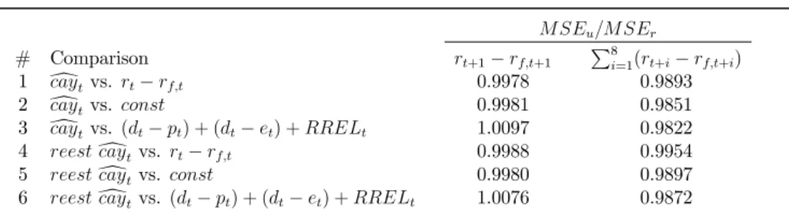
). Tabela 6 presents the results for nested regressions. From Tabela 6,
it is clear that adding cayL to the benchmark models always decrease the MSFE of the regressions on a two-year horizon. This happens whether the cointegrating coefficients are re-estimated or not. For one quarter ahead,cayL andreestcayL also do better than the constant and lagged benchmarks, but not when we includedt−pt,dt−et, andRRELt. Again, the benefit of addingcayL in these regressions is greater over the two years accumulated excess returns, which is consistent with the results from long-term regressions above.
In Tabela 7, we extend our analysis by making nonnested forecasts. Compared to the financial vari-ables,cayL produces superior forecasts regardless of whether its coefficients are re-estimated or whether we want to predict the next quarter or two years accumulated excess returns. The strength ofcayL as a predictor may be noticed specially with regard to the payout ratio, d−e. However, when making
12The tests consist of running regressions with different lags,l, of the form
(r t−rf,t
)
=α0+α1(rt−1−rf,t−1
)
+· · ·+αl(rt−l−rf,t−l
)
Table 6.Out-of-sample nested comparisons.
M SEu=M SEr
# Comparison rt+1 rf;t+1 P
8
i=1(rt+i rf;t+i)
1 dcaytvs. rt rf;t 0.9978 0.9893
2 dcaytvs. const 0.9981 0.9851
3 dcaytvs. (dt pt) + (dt et) +RRELt 1.0097 0.9822
4 reestdcaytvs. rt rf;t 0.9988 0.9954
5 reestdcaytvs. const 0.9980 0.9897
6 reestdcaytvs. (dt pt) + (dt et) +RRELt 1.0076 0.9872
Notes:This table shows the results of the nested comparisons, displaying the MSE ratio from the unrestricted model, which includes eithercayL orreestcayL, over the restricted model without this variables. The first valued column refers to one-quarter-ahead excess returns forecasts and the second one refers to two years accumulated excess returns predictions. The first three rows are computed withcayL estimated from the full sample and the last three with its parameters recursively re-estimated (reestcayL).
Table 7.Out-of-sample nonnested comparisons.
M SE1=M SE2
# Comparison rt+1 rf;t+1 P
8
i=1(rt+i rf;t+i)
1 dcayt vs. rt rf;t 1.0032 0.9862
2 dcayt vs. dt pt 0.9956 0.9938
3 dcayt vs. dt et 0.9822 0.9616
4 dcayt vs. RRELt 0.9863 0.9874
5 reestdcaytvs. rt rf;t 1.0035 0.9915 6 reestdcaytvs. dt pt 0.9959 0.9992 7 reestdcaytvs. dt et 0.9825 0.9668 8 reestdcaytvs. RRELt 0.9866 0.9928
Notes:This table reports the results of nonnested comparisons, displaying the MSE ratio from the first model, with eithercayL orreestcayL as the sole predictor, over the second model, with financial variables or lagged excess returns. Once more, the first valued col-umn refers to one-quarter-ahead excess returns forecasts and the second one refers to two years accumulated excess returns predictions. The first four rows are computed withcayL es-timated from the full sample and the last two with its parameters recursively re-eses-timated.
forecasts over one quarter ahead, both cayL andreestcayL produce higher MSFEs in relation to lagged excess returns. Except forRREL, the impact ofcayL andreestcayL over the MSFE ratio is greater for two years accumulated excess returns. At this time length, the forecasting power ofcayL even overcomes the predictive power of lagged excess returns. Moreover, comparing the first four rows with the last four, we see thatcayL has a superior forecasting power than its re-estimated version, as one would expect.
All in all, we find thatcayL beats most alternatives across both horizons investigated here. Out-of-sample results are consistent with the in-sample results as a whole, confirming the predictability of
L
7. COINTEGRATION AND FORECASTING WITH A FMOLS ESTIMATE OF
cay
As pointed out in the Introduction, from a theoretical perspective, the cointegrating vector should be
cayt=(1,−γ,−(1−γ))*...
, ct at yt
+/ //
-,
where0≤γ≤1should be the share of asset wealth in total wealth. However, inspection of our empirical
results in section 4 and the Appendices, shows that not always these theoretical restrictions were obeyed. Two possible reasons for that are measurement error on the components of cayt or the fact that we obtain the present-value equation (11) using a first-order log-linear approximation.
Lettau & Ludvigson (2001) and some subsequent papers in the literature also present these prob-lems, especially the fact that coefficients did not add up to unity, which was not viewed as major issue. So, we follow the early literature and try to estimate the cointegrating vector using a method that could in principle yield estimates of the homogeneous cointegrating vector(
1,−βa,−βy), where0≤βa,βy≤1, with an analogous restriction binding also for the heterogeneous case. However, we do not impose that βa+βy=1. To implement that, we apply the Fully Modified Ordinary Least Squares (FMOLS) proposed by Phillips & Hansen (1990). This approach, in contrast to the standard OLS, eliminates problems of asymptotic bias of the estimates caused by the long run correlation between the cointegrating equation and stochastic regressors innovations. This allows inference on the cointegrating vector.
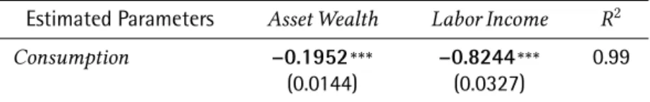
Tabela 8 reports the results on the homogeneous cointegrating vector, obtained from the FMOLS for the entire panel. In Appendix B, we present the heterogeneous vectors results, derived from the time-series FMOLS regressions estimated separately for each country.
Table 8.Panel homogeneous cointegrating vector.
Estimated Parameters Asset Wealth Labor Income R2
Consumption −0.1952*** −0.8244*** 0.99
(0.0144) (0.0327)
Notes: This table presents the estimated parameters of the cointegrating vector (1,−βDy,−βDa)from the FMOLS estimation, with respective standard errors in parenthesis. On the specification, we include an intercept in the cointegrating equation. 601 observations are included in this estimation after adjustments. Both estimates are statistically significant at 1% level (***), computed using asymptoticχ2distribution.
For the homogeneous cointegrating vector, contrary to previous results, we now do not observe a negative share for human-capital wealth. Also, for the heterogeneous case, we only observed two in-stances with negative shares for asset wealth (France and the UK), which are very small numerically and statistically insignificant. Thus, from a practical and statistical point-of-view, our FMOLS cointegrating vectors are theoretically valid.
With these new results in hand, we buildcayLf, the homogeneous version of the cointegrating residual using FMOLS, andcayLf h, its heterogenous counterpart. Once again, we check the stationarity of cayLf and cayLf h by performing the Fisher-ADF and PP panel unit root tests, including individual intercepts but not any trends. For both variables, the presence of unit root is strongly rejected on both ADF and PP tests, confirming their stationarity.
Figure 2.Excess Returns and Estimatedcay.
the year of 2013, the excess returns of France, Italy, Japan and United Kingdom have already followed the latest cayLf swings. On the other hand, United States and Canada still show opposite movements between those two variables. Thus, if cayLf is indeed a good predictor of excess returns, we should expect a decline in excess return’s path in the next few quarters of 2014 and 2015 for both Canada and United States.
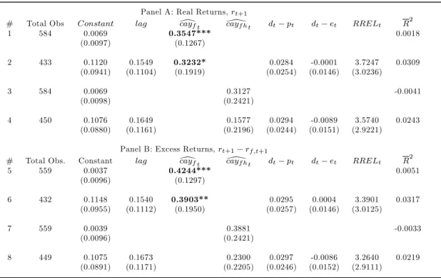
Next, we perform the in-sample one-quarter-ahead predictability tests usingcayLf orcayLhf. Re-sults are presented in Tabela 9. Contrary to previous reRe-sults, now, bothcayLf andcayLf h can significantly forecast one-quarter-ahead stock returns and excess returns. But, other financial variables included in the regressions cannot.
Tabela 10 we presents the results of forecasting tests for in-sample long-term regressions, investi-gating the impact ofcayLf and cayLf h over accumulated consumption growth and accumulated excess returns.
From Panel A on Tabela 10 we notice thatcayLf h is a better predictor of consumption growth than L
cayf, based on a larger adjustedR2. In contrast, in Panel B,cayL
f is a better predictor overall. Comparing
L
cayf with the other financial variables (rows 4 and 5)cayLf is a much better predictor of excess returns thand−p, except for a horizon of six years. The same is not true for the payout ratio, on row 6. On
Table 9. In-sample one-quarter-ahead regressions.
Panel A: Real Returns,rt+1
# Total Obs Constant lag cay[f t cay\f ht dt pt dt et RRELt R
2
1 584 0.0069 0.3547*** 0.0018
(0.0097) (0.1267)
2 433 0.1120 0.1549 0.3232* 0.0284 -0.0001 3.7247 0.0309
(0.0941) (0.1104) (0.1919) (0.0254) (0.0146) (3.0236)
3 584 0.0069 0.3127 -0.0041
(0.0098) (0.2421)
4 450 0.1076 0.1649 0.1577 0.0294 -0.0089 3.5740 0.0243
(0.0880) (0.1161) (0.2196) (0.0244) (0.0151) (2.9221)
Panel B: Excess Returns,rt+1 rf;t+1
# Total Obs. Constant lag cay[f t cay\f ht dt pt dt et RRELt R
2
5 559 0.0037 0.4244*** 0.0051
(0.0096) (0.1297)
6 432 0.1148 0.1540 0.3903** 0.0295 0.0004 3.3901 0.0317
(0.0955) (0.1112) (0.1950) (0.0257) (0.0146) (3.0125)
7 559 0.0039 0.3881 -0.0033
(0.0096) (0.2421)
8 449 0.1075 0.1673 0.2300 0.0297 -0.0086 3.2640 0.0219
(0.0891) (0.1171) (0.2205) (0.0246) (0.0152) (2.9111)
Notes:This table shows some regressions of one-step-forward returns forecasts. Total Obs. refers to the total panel unbalanced observations included after adjustments, andlagis the one-lag backward dependent variable, i.e. ont, used as a regressor. The Constant is an overall fixed effects mean and we omit the specific fixed effects of each country. The last column reports the adjustedR2. White cross-section corrected standard errors appear in parenthesis. Statistics with* are significant at 10% level,
**at 5% and***at 1%.
considered a good predictor.
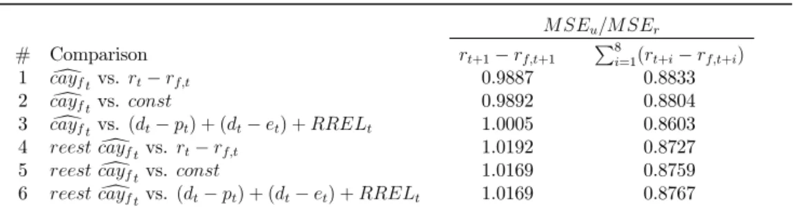
Tabela 11 presents the results of the out-of-sample forecasting exercise for excess returns. Again, we make both nested and nonnested comparisons and use either cayLf or reestcayLf, which has its coefficients recursively re-estimated using FMOLS.
At the one-quarter-ahead horizon, results forreestcayLf in Tabela 11 are disappointing, butcayLf still beats lagged excess returns and the constant-return model. For the accumulated excess returns up to two years ahead, bothcayLf orreestcayLf forecast much better than any of the alternatives. The decrease in MSFE can reach up to 14%, which is impressive compared to previous results.
Tabela 12 present the results of the non-nested tests. For accumulated excess returns, note that
L
cayf orreestcayLf produce superior forecasts than any other alternative predictor. For one-step-ahead, the same can be said aboutcayLf, with an excellent out-of-sample performance beating alternative pre-dictors by more than 15%. However,reestcayLf is beaten almost by all alternative predictors, with the exception ofd−e.
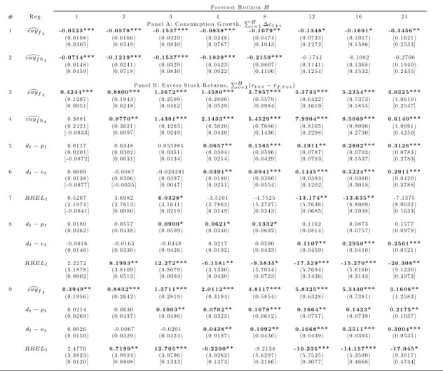
impos-Table 10.In-sample long-horizon regressions.
Fo re c a st H o riz o nH
# R e g . 1 2 3 4 8 1 2 1 6 2 4
P a n e l A : C o n su m p tio n G row th ,PH i=1 ct+i
1 cay[f t - 0 .0 3 2 3 * * * - 0 .0 5 7 8 * * * - 0 .1 5 3 7 * * * - 0 .0 8 3 8 * * * - 0 .1 0 7 9 * * - 0 .1 3 4 8 * - 0 .1 6 9 1 * - 0 .3 4 5 6 * * (0 .0 1 0 8 ) (0 .0 1 6 6 ) (0 .0 3 2 9 ) (0 .0 2 4 8 ) (0 .0 4 7 4 ) (0 .0 7 3 3 ) (0 .1 0 1 7 ) (0 .1 6 2 1 ) [0 .0 3 0 5 ] [0 .0 5 4 9 ] [0 .0 8 3 0 ] [0 .0 7 6 7 ] [0 .1 0 4 3 ] [0 .1 2 7 2 ] [0 .1 5 8 6 ] [0 .2 5 3 3 ]
2 cay\f h t - 0 .0 7 1 4 * * * - 0 .1 2 1 9 * * * - 0 .1 5 3 7 * * * - 0 .1 8 3 9 * * * - 0 .2 1 5 9 * * * -0 .1 7 4 1 -0 .1 0 8 2 -0 .2 7 0 0 (0 .0 1 4 8 ) (0 .0 2 4 1 ) (0 .0 3 2 9 ) (0 .0 4 2 3 ) (0 .0 8 0 7 ) (0 .1 1 4 1 ) (0 .1 3 6 8 ) (0 .1 9 4 0 ) [0 .0 4 5 9 ] [0 .0 7 1 8 ] [0 .0 8 3 0 ] [0 .0 9 2 2 ] [0 .1 1 0 6 ] [0 .1 2 5 4 ] [0 .1 5 3 2 ] [0 .2 4 3 5 ]
P a n e l B : E x c e ss S to ck R e tu rn s,PH
i=1(rt+i rf;t+i)
3 cay[f t 0 .4 2 4 4 * * * 0 .8 8 0 0 * * * 1 .3 6 7 2 * * * 1 .4 5 8 0 * * * 3 .7 8 5 7 * * * 5 .3 7 3 3 * * * 5 .2 3 5 4 * * * 3 .0 3 2 5 * * * (0 .1 2 9 7 ) (0 .1 9 4 3 ) (0 .2 5 0 9 ) (0 .2 8 0 0 ) (0 .5 5 7 9 ) (0 .6 4 2 2 ) (0 .7 3 7 3 ) (1 .0 6 1 0 ) [0 .0 0 5 1 ] [0 .0 2 4 8 ] [0 .0 4 6 2 ] [0 .0 5 2 9 ] [0 .0 9 8 4 ] [0 .1 6 1 9 ] [0 .1 8 5 5 ] [0 .2 5 4 7 ]
4 cay\f h t 0 .3 8 8 1 0 .8 7 7 0 * * 1 .4 3 8 1 * * * 2 .1 4 3 3 * * * 5 .4 5 2 9 * * * 7 .9 9 0 4 * * * 8 .5 0 6 9 * * * 6 .6 1 4 0 * * * (0 .2 4 2 1 ) (0 .3 6 2 1 ) (0 .4 2 6 5 ) (0 .5 0 2 0 ) (0 .7 6 8 6 ) (0 .8 1 0 5 ) (0 .8 0 9 0 ) (1 .0 6 9 1 ) [-0 .0 0 3 3 ] [0 .0 0 9 7 ] [0 .0 2 4 9 ] [0 .0 4 4 0 ] [0 .1 4 3 6 ] [0 .2 2 9 8 ] [0 .2 7 3 0 ] [0 .4 2 5 0 ]
5 dt pt 0 .0 1 1 7 0 .0 3 4 8 0 .0 5 5 9 8 5 0 .0 6 5 7 * * 0 .1 5 8 5 * * * 0 .1 9 1 1 * * 0 .2 8 0 2 * * * 0 .3 1 2 6 * * * (0 .0 2 0 1 ) (0 .0 3 0 2 ) (0 .0 3 5 1 ) (0 .0 3 0 4 ) (0 .0 5 9 6 ) (0 .0 7 8 7 ) (0 .0 7 0 3 ) (0 .0 7 8 3 ) [-0 .0 0 7 2 ] [0 .0 0 3 1 ] [0 .0 1 3 4 ] [0 .0 2 1 4 ] [0 .0 4 2 9 ] [0 .0 7 8 3 ] [0 .1 5 3 7 ] [0 .2 7 8 3 ]
6 dt et 0 .0 0 0 9 -0 .0 0 8 7 -0 .0 2 0 3 9 1 0 .0 3 9 1 * * 0 .0 9 4 1 * * * 0 .1 4 4 5 * * * 0 .3 2 2 4 * * * 0 .2 9 1 1 * * * (0 .0 1 3 8 ) (0 .0 3 0 6 ) (0 .0 3 9 7 ) (0 .0 1 8 0 ) (0 .0 3 6 0 ) (0 .0 3 9 3 ) (0 .0 3 6 0 ) (0 .0 4 2 0 ) [-0 .0 0 7 7 ] [-0 .0 0 3 5 ] [0 .0 0 4 7 ] [0 .0 2 5 1 ] [0 .0 5 5 4 ] [0 .1 2 0 2 ] [0 .3 0 1 8 ] [0 .3 7 8 8 ]
7 RRELt 0 .5 2 0 7 3 .6 9 8 2 6 .0 3 2 8 * -3 .5 1 0 1 -4 .7 5 2 5 - 1 3 .1 7 4 * * - 1 3 .6 3 5 * * -7 .1 3 7 5 (2 .1 0 7 4 ) (2 .7 6 1 3 ) (3 .1 6 4 1 ) (2 .7 8 6 2 ) (5 .2 7 2 7 ) (5 .7 6 3 6 ) (6 .8 0 0 9 ) (8 .0 0 3 2 ) [-0 .0 0 4 1 ] [0 .0 0 8 6 ] [0 .0 2 1 9 ] [0 .0 1 4 9 ] [0 .0 2 4 3 ] [0 .0 6 8 5 ] [0 .1 0 3 8 ] [0 .1 6 3 3 ]
8 dt pt 0 .0 1 8 0 0 .0 5 5 7 0 .0 9 0 0 * 0 .0 6 2 1 * 0 .1 3 3 2 * 0 .1 1 6 2 0 .0 8 7 3 0 .1 5 7 7 (0 .0 2 6 2 ) (0 .0 4 3 8 ) (0 .0 5 0 9 ) (0 .0 3 4 0 ) (0 .0 6 9 2 ) (0 .0 8 1 4 ) (0 .0 7 5 7 ) (0 .0 9 7 9 )
dt et -0 .0 0 1 6 -0 .0 1 6 5 -0 .0 3 4 8 0 .0 2 1 7 0 .0 5 9 0 0 .1 1 0 7 * * 0 .2 9 5 0 * * * 0 .2 5 6 1 * * * (0 .0 1 4 6 ) (0 .0 3 3 0 ) (0 .0 4 2 6 ) (0 .0 1 9 2 ) (0 .0 4 3 3 ) (0 .0 4 5 9 ) (0 .0 4 1 0 ) (0 .0 5 2 1 )
RRELt 2 .2 2 7 2 8 .1 9 9 3 * * 1 2 .2 7 2 * * * - 6 .1 5 8 1 * * - 9 .5 8 3 5 * - 1 7 .3 2 9 * * * - 1 5 .2 7 0 * * * - 2 0 .3 0 8 * * (3 .1 8 7 8 ) (3 .8 1 0 9 ) (3 .8 6 7 9 ) (3 .1 3 3 0 ) (5 .7 0 5 4 ) (5 .7 6 9 4 ) (5 .6 1 6 0 ) (9 .1 2 3 0 ) [0 .0 0 0 2 ] [0 .0 5 1 3 ] [0 .0 9 0 3 ] [0 .0 4 3 0 ] [0 .0 7 2 3 ] [0 .1 4 3 6 ] [0 .3 1 4 3 ] [0 .3 9 7 2 ]
9 cay[f t 0 .3 9 4 9 * * 0 .8 8 3 2 * * * 1 .3 7 1 1 * * * 2 .0 1 1 2 * * * 4 .8 1 1 7 * * * 5 .8 3 2 5 * * * 5 .3 4 4 0 * * * 3 .1 6 0 8 * * (0 .1 9 5 6 ) (0 .2 6 4 2 ) (0 .2 8 1 9 ) (0 .3 1 9 4 ) (0 .5 8 5 4 ) (0 .6 3 2 8 ) (0 .7 3 8 1 ) (1 .2 5 8 3 )
dt pt 0 .0 2 1 4 0 .0 6 3 0 0 .1 0 0 3 * * 0 .0 7 6 2 * * 0 .1 6 7 8 * * * 0 .1 6 6 4 * * 0 .1 4 2 3 * 0 .2 1 7 5 * * (0 .0 2 6 9 ) (0 .0 4 3 7 ) (0 .0 4 9 6 ) (0 .0 3 2 2 ) (0 .0 6 1 2 ) (0 .0 7 5 7 ) (0 .0 7 3 9 ) (0 .1 0 3 7 )
dt et 0 .0 0 2 6 -0 .0 0 6 7 -0 .0 2 0 1 0 .0 4 3 8 * * 0 .1 0 9 2 * * 0 .1 6 6 8 * * * 0 .3 5 1 1 * * * 0 .3 0 0 4 * * * (0 .0 1 5 0 ) (0 .0 3 2 9 ) (0 .0 4 2 4 ) (0 .0 1 9 7 ) (0 .0 4 3 6 ) (0 .0 4 3 9 ) (0 .0 3 9 3 ) (0 .0 5 3 5 )
RRELt 2 .4 7 7 0 8 .7 1 9 9 * * 1 2 .7 0 5 * * * - 6 .2 2 0 0 * * -9 .2 1 3 8 - 1 6 .2 3 5 * * * - 1 4 .1 5 7 * * * - 1 7 .0 4 5 * (3 .3 8 2 3 ) (3 .9 9 2 4 ) (3 .9 7 9 6 ) (3 .0 2 6 2 ) (5 .6 2 9 7 ) (5 .7 5 2 5 ) (5 .3 5 9 0 ) (9 .3 0 1 7 ) [0 .0 1 2 0 ] [0 .0 8 0 8 ] [0 .1 3 3 3 ] [0 .1 3 7 3 ] [0 .2 1 8 6 ] [0 .3 0 7 7 ] [0 .4 6 6 6 ] [0 .4 7 3 4 ]
Notes: This table reports estimates from the long-horizon regressions of accumulated consumption growth and accumulated excess stock returns oncayLf,cayLf hand the financial variables. We omit the constants of all regressions. “Reg.” indicates the regressors included in each regression. The forecast horizon length is in quarters. White cross-section corrected standard errors are displayed in parenthesis andR2are in brackets at the end of each regression. Statistics with *are significant at 10% level,
**at 5% and***at 1%.
ing a fully-fledged theoretical model, although an intermediately restricted model produced forecasting winners more frequently.
8. CONCLUSIONS
Table 11.Out-of-sample nested comparisons.
M SEu=M SEr
# Comparison rt+1 rf;t+1 P
8
i=1(rt+i rf;t+i)
1 caydf tvs. rt rf;t 0.9887 0.8833
2 caydf tvs. const 0.9892 0.8804 3 caydf tvs. (dt pt) + (dt et) +RRELt 1.0005 0.8603
4 reestcaydf t vs.rt rf;t 1.0192 0.8727
5 reestcaydf t vs.const 1.0169 0.8759 6 reestcaydf t vs.(dt pt) + (dt et) +RRELt 1.0169 0.8767
Notes:This table shows the results of the nested comparisons, displaying the MSE ratio from the unrestricted model, which includes eithercayLf orreestcayLf, over the restricted model, without these variables. The first value column refers to one-quarter-ahead excess returns forecasts and the second one refers to two years accumulated excess returns predictions. The first three rows are computed withcayLf estimated from the full sample and the last three with its parameters recursively re-estimated (reestcayLf).
Table 12.Out-of-sample nonnested comparisons.
M SE1=M SE2
# Comparison rt+1 rf;t+1
P8
i=1(rt+i rf;t+i)
1 caydf tvs.rt rf;t 0.9916 0.8798
2 caydf tvs.dt pt 0.9841 0.8866
3 caydf tvs.dt et 0.9708 0.8578
4 caydf tvs.RRELt 0.9748 0.8809
5 reestcaydf tvs.rt rf;t 1.0192 0.8695 6 reestcaydf tvs.dt pt 1.0116 0.8762 7 reestcaydf tvs.dt et 0.9979 0.8477 8 reestcaydf tvs.RRELt 1.0020 0.8706
Notes:This table reports the results of nonnested comparisons, displaying the MSE ratio from the first model, withcayLf as the sole predictor, over the second model, with financial variables or lagged excess returns. Once more, the first valued column refers to one-quarter-ahead excess returns forecasts and the second one refers to two years accumulated excess returns predictions. The first four rows are computed withcayLf estimated from the full sample and the last two with its parameters recursively re-estimated.
We employ macroeconomic and financial quarterly data for the group of G7 countries, forming an unbalanced panel. For most countries, data is available from the early 1990s until 2014Q1, but for the U.S. economy it is available from 1981Q1 through 2014Q1. Our final results allowed a very broad examination of the present-value theory behindcay, which conclusions we list below:
1. We find overwhelming evidence of a single cointegration vector for consumption, asset wealth, and labor income, in formingcay.
2. In some cases, the coefficients in the cointegrating linear combination did not conform to theory, since they must lie between zero and one and add up to unity. This issue required alternative estimation techniques and forecast evaluation.
4. Estimates of cay help to forecast future stock returns and excess returns in the out-of-sample exercise, usually performing better than alternative regressors.
5. Finally, using estimates ofcaythat conform to economic theory does improve forecasts of future accumulated excess returns up to the two-year horizon.
All in all, we believe that our evidence has shown that the predictive power ofcayis not a phe-nomenon restricted to the U.S. economy, but a much wider phephe-nomenon, which deserves to be studied more broadly.
REFERENCES
Arellano, M. (1987). Computing robust standard errors for within-groups estimators.Oxford Bulletin of Economics
and Statistics,49(4), 431–434.
Campbell, J. Y. (1987). Does saving anticipate declining labor income? An alternative test of the permanent income
hypothesis.Econometrica,55(6), 1249–1273.
Campbell, J. Y. (1996). Understanding risk and return.Journal of Political Economy,104(2), 298–345.
Campbell, J. Y., & Deaton, A. (1989). Why is consumption so smooth? The Review of Economic Studies,56(3),
357–373.
Campbell, J. Y., & Mankiw, N. G. (1989). Consumption, income and interest rates: Reinterpreting the time series
evidence. In O. J. Blanchard & S. Fischer (Eds.),NBER Macroeconomics Annual 1989, Volume 4(pp. 185–246).
MIT Press. Retrieved from http://www.nber.org/chapters/c10965
Campbell, J. Y., & Shiller, R. J. (1987). Cointegration and tests of present value models.Journal of Political Economy,
95(5), 1062–1088.
Campbell, J. Y., & Shiller, R. J. (1988a). The dividend-price ratio and expectations of future dividends and discount
factors.The Review of Financial Studies,1(3), 195–228.
Campbell, J. Y., & Shiller, R. J. (1988b). Stock prices, earnings, and expected dividends. Journal of Finance,43(3), 661–76.
Campbell, J. Y., & Thompson, S. B. (2008). Predicting excess stock returns out of sample: Can anything beat the
historical average? The Review of Financial Studies,21(4), 1509–1531.
Engle, R. F., & Granger, C. W. J. (1987). Co-integration and error correction: Representation, estimation, and testing.
Econometrica,55(2), 251–276.
Fama, E. F., & French, K. R. (1988). Dividend yields and expected stock returns. Journal of Financial Economics,
22(1), 3–25.
Fisher, R. A. (1932).Statistical methods for research workers(4th ed.). Edinburgh: Oliver and Boyd.
Gao, P. P., & Huang, K. X. (2008). Aggregate consumption-wealth ratio and the cross-section of stock returns: Some
international evidence.Annals of Economics and Finance,9(1), 1–37.
Guillén, O. T. a. H., Issler, J. V., & Saraiva, D. (2015). Forecasting multivariate time series under present-value model
short- and long-run co-movement restrictions.International Journal of Forecasting,31(3), 862–875.
Hodrick, R. J. (1992). Dividend yields and expected stock returns: Alternative procedures for interference and
measurement.Review of Financial Studies,5(3), 357–386.
Ioannidis, C., Peel, D., & Matthews, K. (2006). Expected stock returns, aggregate consumption and wealth: Some
further empirical evidence.Journal of Macroeconomics,28(2), 439–445.
Johansen, S. (1991). Estimation and hypothesis testing of cointegration vectors in Gaussian vector autoregressive
Judson, R. A., & Owen, A. L. (1999). Estimating dynamic panel data models: A guide for macroeconomists. Eco-nomics Letters,65(1), 9–15.
Kao, C. (1999). Spurious regression and residual-based tests for cointegration in panel data.Journal of
Economet-rics,90(1), 1–44.
Lamont, O. (1998). Earnings and expected returns.Journal of Finance,53(5), 1563–1587.
Lettau, M., & Ludvigson, S. (2001). Consumption, aggregate wealth, and expected stock returns. Journal of
Finance,56(3), 815–849.
Lettau, M., & Ludvigson, S. C. (2004). Understanding trend and cycle in asset values: Reevaluating the wealth
effect on consumption.American Economic Review,94(1), 276–299.
Maddala, G. S., & Wu, S. (1999). A comparative study of unit root tests with panel data and new simple test.
Oxford Bulletin of Economics and Statistics,Special Issue 61, 631–652.
Nickell, S. J. (1981). Biases in dynamic models with fixed effects.Econometrica,49(6), 1417–1426.
Nitschka, T. (2010). International evidence for return predictability and the implications for long-run covariation
of the G7 stock markets.German Economic Review,11, 527–544.
Pesaran, M. H., & Timmermann, A. (1995). Predictability of stock returns: Robustness and economic significance.
Journal of Finance,50(4), 1201–1228.
Phillips, P. C. B., & Hansen, B. E. (1990). Statistical inference in instrumental variables regression withI(1)
processes.Review of Economic Studies,57(1), 99–125.
Sousa, R. M. (2010). Consumption, (dis)aggregate wealth, and asset returns. Journal of Empirical Finance,17(4),
606–622.
Tsuji, C. (2009). Consumption, aggregate wealth, and expected stock returns in Japan. International Journal of
Economics and Finance,1(2), 123–133.
APPENDIX A. VECM HETEROGENEOUS COINTEGRATING VECTORS
This appendix provides the results from the VEC regressions for each country separately. Tabela A-1 shows the cointegrating vector parameters estimates when we relax the homogeneity restrictions, lead-ing to heterogeneous coefficients among countries. On every VEC specification, we include an intercept in the cointegrating equation, we use one lag in difference for the endogenous variables and impose on cointegrating relationship among them.
With these estimated parameters we construct the variable cayLh, which represents the cointe-grating residual when we allow for heterogeneity on coefficients, just as we describe in section 4.
Table A-1.Heterogeneous cointegrating vectors.
Estimated Parameters AssetW ealth LaborIncome Constant
Consumption
Canada 1.0091*** -3.0200*** 9.5197
(0.2245) (0.4719)
France 0.7842*** -2.7832*** 6.4006
(0.1925) (0.3837)
Germany -0.2011*** -0.4126*** -2.7835
(0.0107) (0.0772)
Italy -0.1789 0.5172 -10.4017
(0.1215) (0.3965)
Japan -0.3486*** -0.3826*** -2.0229
(0.0331) (0.0709)
United Kingdom -0.1073** -0.8947*** 0.0846
(0.0452) (0.0451)
United States -0.6898*** 0.1587 -2.1200
(0.23672) (0.4907)
Notes: This table presents the estimated parameters of the cointegrating vectors (1
,−βDy,i,−βDa,i
APPENDIX B. FMOLS HETEROGENEOUS COINTEGRATING VECTORS
This appendix provides the results from the FMOLS regressions for each country separately. Tabela B-2 shows the cointegrating vector parameters estimates when we relax the homogeneity restrictions, leading to heterogeneous coefficients among countries. In addition, in the specification, we include distinct constants in the cointegrating structure for each country.
With these estimated parameters we construct the variablecayLf h, which represents the cointe-grating residual when we allow for heterogeneity on coefficients, just as we describe in section 7.
Table B-2.Heterogeneous cointegrating vectors.
Estimated Parameters AssetW ealth LaborIncome Constant R2
Consumption
Canada -0.2322*** -0.5455*** 0.4957 0.99
(0.0324) (0.0695) (0.3412)
France 0.0008 -0.9523*** 0.4770* 0.97
(0.0381) (0.0694) (0.2856)
Germany -0.1931*** -0.3664*** 3.2525*** 0.95
(0.0087) (0.0575) (0.4430)
Italy -0.2874*** -0.1677* 3.8119*** 0.89
(0.0339) (0.0995) (0.5481)
Japan -0.3107*** -0.3372*** 3.298*** 0.76
(0.0272) (0.0606) (1.2337)
United Kingdom 0.0006 -0.8837*** 1.1555*** 0.97
(0.0286) (0.0267) (0.4118)
United States -0.4810*** -0.4591** -1.4607 0.96
(0.1046) (0.2180) (0.9745)
Notes: This table presents the estimated parameters of the cointegrating vectors (
1,−βDy,i,−Dβa,i