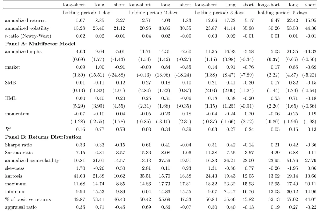
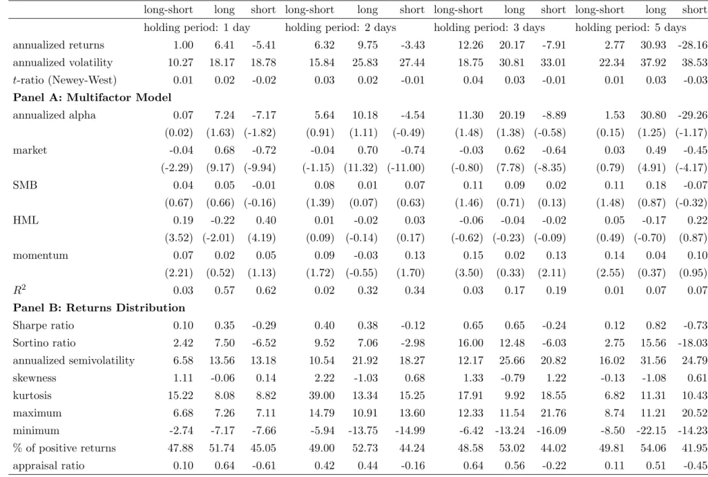
Conditional alphas and realized betas

For examining the discourses of citizens and representatives of expert-political systems regarding public participation within processes of participatory budgeting, we selected

Esta pesquisa teve como objetivo estudar A Problemática do Destino Final dos Resíduos Sólidos no Município de São José do Campestre-RN, buscando identificar o crescimento da

Na figura 6.1 é possível ver a modelação do veio e do rolo, assim como as condições iniciais deste estudo, onde foram aplicados os deslocamentos na ponta do rolo

Já em função da taxa de cisalhamento, a viscosidade rotacional apresenta um comportamento newtoniano para baixas taxas, quando não são consideradas interações entre as partículas..

Num segundo momento e de forma interpenetrada, realizou-se a interpretação dos relatos tomando-se como categorias de análise as estruturas sociais que objetivam a relação e

Características avaliadas na cultura do repolho tratada com diferentes produtos a base Bacillus thuringiensis para o controle de traça-das-crucíferas, EmbrapaBrasília-DF/2003..

This thesis examines, in the framework of the common ingroup identity model, the effectiveness of different types of superordinate category to reduce intergroup

Avec l’exotisme du XIX ème siècle, on retrouve de plus en plus un type d’exotisme de premier degré dans lequel l’étrangeté non- européenne n’est pas diminuée comme