http://dx.doi.org/10.4236/jamp.2014.28084
Taylor’s Power Law for Ecological
Communities
—
An Explanation on
Nonextensive/Nonlinear Statistical Grounds
João D. T. Arruda-Neto
1,2, Henriette Righi
1, Marcos Antonio G. Cascino
2,
Godofredo C. Genofre
2, Joel Mesa
31
Instituto de Física, Universidade de São Paulo, São Paulo, Brasil
2CEPESq, Centro Universitário Ítalo-Brasileiro, São Paulo, Brasil 3São Paulo State University, UNESP, Botucatu, Brasil
Email: [email protected]
Received 24 April 2014; revised 20 May 2014; accepted 3 June 2014 Copyright © 2014 by authors and Scientific Research Publishing Inc.
This work is licensed under the Creative Commons Attribution International License (CC BY).
http://creativecommons.org/licenses/by/4.0/
Abstract
A new idea on how to conceptually interpret the so-called Taylor’s power law for ecological com-munities is presented. The core of our approach is based on nonextensive/nonlinear statistical concepts, which are shown to be at the genesis of all power laws, particularly when a system is constituted by long-range interacting elements. In this context, the ubiquity of the Taylor’s power law is discussed and addressed by showing that long-range interactions are at the heart of the in-ternal dynamics of populations.
Keywords
Taylor’s Law, Long-Range Interaction, Population Variabilities, Ecological Complexity, Ecological Nonlinearity
1. Introduction
Nearly 35 years ago, Taylor and collaborators proposed the so-called Taylor’s model, based on the analysis of 156 sets of data from a wide range of species and sampling scales (from ciliates on the surface of a flat-worm to the human population of the United States of America). The model assumed that spatial variance (V) is propor-tional to a fracpropor-tional power of the mean population density (M), that is [1]
which can be represented by log-log plots as
logV =logα β+ logM (2) where α is a proportionality parameter and βwas regarded as an index of aggregation, which takes a characteris-tic value for each species, reflecting the balance between opposing behavioral tendencies to move towards or away from centers of population density [1]-[3].
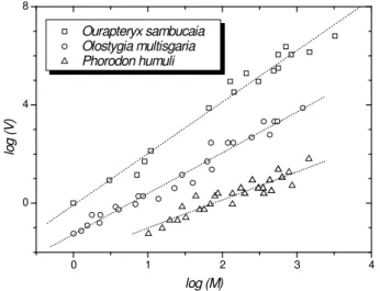
Since then, the relationship between V and M has been established for more than 400 species in the taxa rang-ing from protists to vertebrates (see Figure 1). Although phenomenological interpretations have appeared else-where [4], explanations for (a) the generality of Taylor’s finding, and (b) for the fact that 1 < β< 2, based on “first principles”, are still lacking. More recently, a comprehensive and lucid account by Cohen [5] explains why very different models lead to Taylor’s law. Additionally, he derived both the growth-rate theorem and the Tay-lor’s law from a simple model of exponential population dynamics, also displaying a link between them.
Elucidating the conceptual framework underlying Taylor’s power law, deeply rooted in fundamental princi- ples (as addressed in Section 2.1 below), is quite relevant. In fact, addressing many current ecological problems such as population viability in conservation biology studies, pest dynamics in agriculture, species diversity and stability, and strategies for environmental monitoring, in general, requires a deep understanding of the relation-ship between a population’s variability (V) and its mean abundance (M). Moreover, understanding the facts that control diversity is high on the agenda for ecologists and conservationists, and different factors evidently operate on different scales.
In this sense, here, an interpretation for Taylor’s Power Law based on concepts for nonlinearity and nonex-tensivity is proposed, where the role played by the peculiarities of interactions (short-versus long-range) among the individuals of an ecological community is emphasized.
2. Present Approach
2.1. Complex, Nonextensive Systems
It has been realized that several complex systems exhibit an underlying structure ruled by shared organizing principles [6]. As a result, all parts of the system communicate with each other by means of long-range interac-tions (interconnectivity). The primary signatures of such a peculiarity are power-laws linking variables of the system in a nonlinear way. In this case, extensive statistics is no longer applicable, since the system variables are nonextensive in the sense that the sum of the system parts does not reproduce the whole system.
The issue we are proposing and addressing here is that power-laws naturally emerge when a long-range inte-raction is switched on, with no exception, even for interacting species in an ecological community. This is al-
Figure 1. Log-log plot of species variance (V) as a function of the mean abundance (M): Data points: Ourapteryx sambucaia (a), Olos-tygia multisgaria (b) and Phorodon humuli (c), three insect species. Straight lines: lines fits to the data points-adapted from [4].
0 1 2 3 4
0 4 8
log (
V
)
ready true in systems as small as the DNA molecule [7], to those as large as galaxy conglomerates [8]. Taylor’s Power Law, with its fractionary exponent β (see Equation (1)), is inserted in this nonextensive/nonlinear scena-rio.
If we consider N a random variable (or, an extensive variable) representing population density, with finite mean M and variance V, the scaling N → KN by a constant K that is, by promoting the same change (K) in all the values assumed by N, leads to:
M →KM ≡M′ (3)
Since V ≈
(
N−M)
2, V scales as2
V →K V ≡V′; (4)
therefore,
2 2
V K V
K
V V
′
= = . (5)
Now, if a power-law connects V with M, as in Equation (1), we have that V =αMβ and V′=αM′β; taking the ratio we obtain;
V M KM
K
V M M
β β
β
α α
′= ′ = =
. (6)
Therefore, N is not an extensive variable. It remains to be shown what the nature of the interactions in eco-logical communities is.
2.2. Interactions in Ecological Communities
When modeling population dynamics, the identification of the following interaction categories is necessary [9]: (1) those taking place among the system components and its internal dynamics, and (2) between the system as a whole and the external world. In this last case, interaction is carried out through the interface (boundary condi-tions).
In the first category the following processes may be present: (a) reproduction and death rates driven by genet-ic peculiarities; (b) regulatory processes: responsible for the coordination of population activities within living space and time; (c) competitive processes, particularly when the quantity of available food is limited; and (d) communication processes.
While processes (a) and (b) take place in a small volume, comparative to the total size of the system, (c) and (d), in general, involve larger distances. As shown in the next section, it is precisely these long-range interac-tions that introduce nonlinearities in the system dynamics (as Taylor’s power law).
Unlike systems constituted by unanimated objects, living systems (animal and human species, in particular) have the ability to regulate the range of the interactions among their elements in response to environmental sti-muli. Like some large predatory animals, ancestral humans also acted as groups (long-range interactions) when hunting large prey such as mammoths, but went out solitary (short-range interactions) for small prey such as an-telopes [10].
2.3. Our Approach: Random Walk + Long Range Correlations
In a system constituted of elements interacting by means of short-range forces, each of these elements interacts only with the elements of the system in close proximity to it. This interaction process can be described as a sim-ple random walk. Because of the short-range character of the interaction, each element (which can be treated as a particle) undergoes random jumps to one of its nearest-neighbor sites, where the jump lengths are small. Let’s represent by ri a vector pointing to a nearest-neighbor site; it represents the ithjump of the walk and ri ≈a
is the jump length.
After n jumps, through a length l=na, the net displacement is
1 n
i i=
=
∑
The probability for a particle to undergo a displacement ri is a Gaussian distribution with the average dis-placement r being [11]
1 0. n i i= =
∑
=r r (8)
Let’s now consider the squared displacement
(
)
2 2
1
n n
i i i
i i
r =
= = ⋅
∑
r∑
r r . (9)Since
r r
i⋅
i=
a
2 and r ri⋅ j =0, the mean square displacement in n steps is2 2
r =na =al (since l=na); thus,
2 ~
r l (10)
The result displayed by Equation (10) follows from the assumption that the single jumps ri are uncorrelated, i.e., r ri⋅ j =a2δij, which is fine for short-range interactions, and its linearity expresses the extensive character of the system (the whole is the sum of the parts). However, Equation (10) needs to be modified for long-range interactions. It is plausible that the jumping correlations r ri⋅ j are proportional to some sort of interaction po- tential between positions ri and rj, defined as Vij, which may be written in quite general form as
; ij
i j k V = ′ γ
−
r r
thus,
(
i j)
i j k γ ⋅ = − r r r r (11)
k′ and k are constants. Then, retaking Equation (9), we have for the mean square displacement after n steps
(
)
2 1 1 2 n n i j i j r al > >= +
∑∑
r r⋅ . (12)From this point on, a random walk is assumed taking place in the plane and that 2πrdr, a differential circular strip, is the elemental area for integration. Therefore,
(
)
2π di⋅ j =
∫
i⋅ j ρ r rr r r r , (13)
where we assume that the in-plane density of pairs
(
r ri⋅ j)
, ρ, is constant. Moreover, since it is always possible to promote a coordinate translation such that rj =0, and putting ri ≡r, we get from Equations (11) and (13)2 2
2π 2π d
2 i j
k k
r r r Ar
r γ γ γ ρ ρ γ − − ⋅ = = ≡ −
∫
r r , (14)
and substituting in Equation (12),
2 2 2
1
2 2
n
i
r al Ar −γ al Anr −γ
>
= +
∑
= + . (15)For large l (or large n) and γ <1 the first term, al, becomes small relative to the second term; then (l=na and r=a)
( )
2 2 2
~
r l ≅Bl −γ l −γ ≡lα (16)
where for 1 < α< 2 the system is nonextensive. In the absence of an interaction potential the system is Brow-nian-like, that is, extensive.
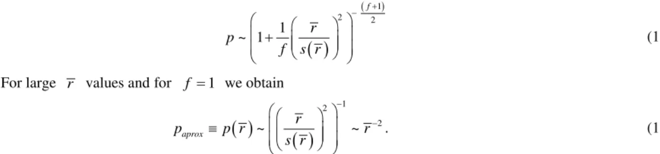
( )
( 1)
2 2 1 ~ 1 f r p
f s r
+ − + (17)
For large r values and for f =1 we obtain
( )
( )
1 2 2 ~ ~ aprox rp p r r
s r − − ≡
. (18)
If the dispersion σ around r is less than 20% (see Figure 2), we can assume r2≅ r2 ~lα (see Equation (16)), and substituting in Equation (18) we obtain
( )
~
p l
l
−α (19)Therefore, it is here demonstrated that a power law emerges from a random walk when an interaction poten-tial between consecutive jumps is introduced. In the present study, the random walk is the random variability of the mean population abundances M (see below).
3. Discussion
3.1. A Nonlinear Ecological Community
On the basis of our nonextensive statistical approach, it is now easy to understand that the ubiquity of Taylor’s power-law slopes in the interval 1 < β < 2 (Equation (1)), is intimately associated with long-range interactions among all the elements of the system. This conclusion is qualitatively correct.
Figure 2. Comparison between p values provided by Equation (17) (dash-curve) and the approxima-tion introduced in Equaapproxima-tion (18) (solid-curve). In the insert the relative difference between the appro- ximate and the exact values is shown. It is salient that for a dispersion of the mean up to approximate-ly 20% (low dispersion), the two distributions are nearapproximate-ly equivalent.
M
0.0 0.1 0.2 0.3 0.4 0.5
0.00 0.05 0.10 0.15 0.20 0.25
0.0 0.1 0.2 0.3 0.4 0.5
0.00 0.05 0.10 0.15 0.20 0.25 ( papr ox - p ) / p
σ / µ
p
aproxp
p
σ
/
Mµ
However, unraveling the peculiarities of such long-range interactions requires modeling, as recently carried out by Kilpatrick and Ives [4]. By using stochastic simulation and analytical models, they demonstrated how ne- gative interactions among species in a community can produce slopes β < 2. There is a key parameter in their model, αij, the competition coefficient giving the per capita effect of species j on species i. The simulations showed that when there are no species competitive interactions (that is, when α =ij 0) the exponent β (Equation (1)) averages 2. Therefore, the population dynamics of single species may be understood in terms of the dynam-ics of a nonextensive or an extensive system, provided these species are interacting or not within their ecological community. Nonlinear selection in natural populations, for instance, has been addressed by Blows and Brooks [13] by means of a complete application of a response surface methodology. Such nonlinearities arise because of the existence of correlation selection on pairs of traits which, in our random walk approach, is the equivalent of having r ri⋅ j ≠0 (see Equations (11) and (14)).
3.2. Probability Distribution of
M
The per capita variability in population abundances (P) is
–1
P =V M =Mβ M =Mβ (20)
We note that the inverse function
–1 1
, with 1
P =M V =M −β =M−δ δ = −b (21)
is proportional to the probability distribution of M, p(M), because the “normalized” behavior (increase or de-crease) of M per unit of variability (that is M/V) is proportional to the probability function of getting a species abundance equal to M. In our working example the function P−1 = P−1(M) indicates that increasingly higher mean population abundances are increasingly less probable. Therefore, p(M) = M−δ (compare with Equation (19)).
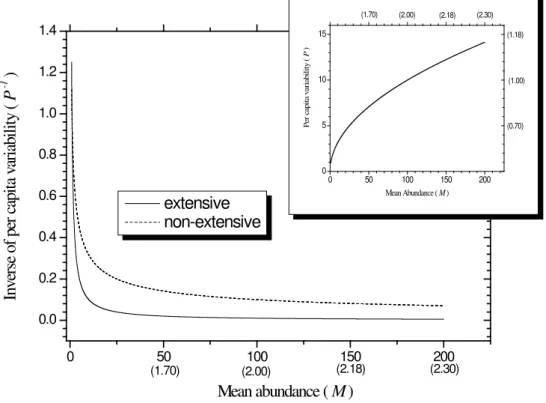
The curves in Figure 3 were obtained from Equation (21) for β = 2 and 1.5, standing for extensive and nonex-tensive,respectively. It is quite salient that for β = 2 the probability for “rare events” is substantially smaller than
Figure 3. Linear-linear plot of the inverse function P−1 as function of M. The numbers in parentheses in the horizontal scale are logM. The solid and dashed curves represent the function given in Equation (21) for β = 2 and 1.5, respectively. In the insert the plot of the per capita variabilityP as function of M is shown.
0 50 100 150 200
0.0 0.2 0.4 0.6 0.8 1.0 1.2 1.4
0 50 100 150 200
0 5 10 15 (1.18) (1.00) (0.70) (2.00) (2.18) (2.30) (1.70) P er c ap ita v ar ia b ility ( P )
Mean Abundance ( M )
(2.30) (2.18) (2.00) (1.70)
In
ver
se o
f p
er
cap
it
a v
ar
iab
il
it
y (
P
-1
)
Mean abundance (
M
)
in the case for β = 1.5. While random outcomes of probabilistic demographic processes generate differences in species characteristics, the long- or short-range character of inter and intra-species interactions determines how their variability responds to increases in abundance.
While the big picture for large M is provided, the nonextensive approach does not alter the small M interval (rare species regime) because the extensive and non-extensive curves converge for M 0. This is, by any means, a nontrivial regime since rare species grow differentially faster than common species and, therefore, move up and out of the rarest abundance categories owing to their rare-species advantage [14]. In fact, estimat-ing the proportion of rare species in particular habitats is a major concern for ecologists. There is, however, no way to achieve effective conservation of both resilience and interconnectivity without the massive input of sci- ence.
In nonextensive scale-free ecological communities (see the Appendix), species are therefore more stable in the sense that, for a given and fixed variance unity, the probability of forming larger populations (see Figure 2) is greater compared to statistically extensive communities. As shown elsewhere [15], computer networks with scale-free architectures, such as the World Wide Web, are not at all prone to accidental failures. Quite revealing in this regard, computer simulations and calculations performed by Albert and Barabási [16] have shown that a growing network with preferential attachment becomes scale-free. This is precisely what was observed in our scale-free networked biological system: growth (increasing M) and preferential attachment (the negative inte-ractions among species). These two ingredients are at the genesis of many other biological system organiza-tions.
In this context, Taylor’s power-law thus showcases a convincing example of nonextensivity in a biological organization, and in our approach the long-range interaction as its key ingredient is identified.
4. Final Remarks
Once it is agreed that an ecological community behaves as a network of interconnected elements, the most pro-found statistical aspects regulating its functioning can be accessed and, as a consequence, new insights for the conception of new models are gotten, while existing ones are improved. Until now, for instance, there has been no analytical derivation of the expected equilibrium distribution of relative species abundance in the local com- munity, and fits to the theory have required simulations [17].
Additionally, as a nonlinear, scale-free network, an ecological community would be entitled to exhibit self- organization (see Appendix), a property lying at the root of life organization itself. In fact, self-organization is the spontaneous emergence of new structures and of new behavior patterns (in animal populations), characteriz- ed by internal feedback links and mathematically described by means of nonlinear equations.
It would appear to us to be a laudable attempt to divulge basic concepts of nonextensivity, and some of their most important applications in life sciences, more widely.
Acknowledgements
This work was supported by grants from FAPESP, CAPES and CNPq, Brazilian funding agencies for the pro-motion of science.
References
[1] Taylor, L.R., Woiwod, I.P. and Perry, J.N. (1978) The Density Dependence of Spatial Behavior and the Rarity of Ran- domness. Journal of Animal Ecology, 47, 383. http://dx.doi.org/10.2307/3790
[2] Taylor, L.R. and Woiwod, I.P. (1980) Temporal Stability as a Density-Dependent Species Characteristic. Journal of Animal Ecology, 49, 209. http://dx.doi.org/10.2307/4285
[3] Taylor, L.R. and Woiwod, I.P. (1982) Comparative Synoptic Dynamics: Relationships between Interspecific and In-traspecific Spatial and Temporal Variance-Mean Population Parameters. Journal of Animal Ecology, 51, 879.
http://dx.doi.org/10.2307/4012
[4] Kilpatrick, A.M. and Ives, A.R. (2003) Species Interactions Can Explain Taylor’s Power Law for Ecological Time Se-ries. Nature, 422, 65. http://dx.doi.org/10.1038/nature01471
[6] Strotz, S.H. (1998) Nonlinear Dynamics and Chaos. Perseus Books.
[7] Bernaola-Galván, P., Román-Roldán, R. and Oliver, J.L. (1996) Compositional Segmentation and Long-Range Fractal Correlation in DNA Sequences. Physical Review E, 53, 5181. http://dx.doi.org/10.1103/PhysRevE.53.5181
[8] Lam, L. (1998) Nonlinear Physics for Beginners. World Scientific, Singapore City. http://dx.doi.org/10.1142/1037
[9] Maynard-Smith, J. (1978) Models in Ecology. Cambridge University Press, Cambridge.
[10] Ridley, M. (1996) The Origins of Virtue. Penguin, London.
[11] Weiss, G.H. (1994) Aspects and Applications of the Random Walk. North Holland, Amsterdam.
[12] Caria, M. (2000) Measurements Analysis: An Introduction to the Statistical Analysis of Laboratory Data in Physics, Chemistry and the Life Sciences. Imperial College Press, London. http://dx.doi.org/10.1142/p196
[13] Blows, M.W. and Brooks, R. (2003) Measuring Nonlinear Selection, American Naturalist, 162, 815. http://dx.doi.org/10.1086/378905
[14] Chave, J., Muller-Landau, H.C. and Levin, S.A. (2002) Comparing Classical Community Models: Theoretical Conse-quences for Patterns of Diversity. American Naturalist, 159, 1. http://dx.doi.org/10.1086/324112
[15] Barabási, A.L. and Bonabeau, E. (2003) Scale-Free Networks. Scientific American, 288, 50. http://dx.doi.org/10.1038/scientificamerican0503-60
[16] Albert, R. and Barabási, A.L. (2002) Statistical Mechanics of Complex Networks. Review of Modern Physics,74, 47. http://dx.doi.org/10.1103/RevModPhys.74.47
[17] Hubbell, S.P. (2001) The Unified Neutral Theory of Biodiversity and Biogeography. Princeton University Press, Prin-ceton.
Appendix: Scale-Invariance and Self-Organization
We can show that the power-law in Equation (1) is, in contemporary parlance, equivalent to the scale-invariant relationship
(
)
( )
V
λ
M
=
λ
βV M
(22)Since λ is arbitrary, we can put λ = 1/M in Equation (22); thus,
( )
( )
1
V M
=
V
M
β≈
M
β (23)that is, Equation (1) is obtained.
Any function V = V(M) satisfying Equation (22) is a homogeneous, scale-invariant function in the sense that if the scale of measuring M, namely, from M to M′ =λM is changed, the new function
V
(
λ
M
′ =
)
λ
βV M
( )
has the same form as V(M).currently publishing more than 200 open access, online, peer-reviewed journals covering a wide range of academic disciplines. SCIRP serves the worldwide academic communities and contributes to the progress and application of science with its publication.
Other selected journals from SCIRP are listed as below. Submit your manuscript to us via either