www.clim-past.net/9/657/2013/ doi:10.5194/cp-9-657-2013
© Author(s) 2013. CC Attribution 3.0 License.
Climate
of the Past
Geoscientiic
Geoscientiic
Geoscientiic
Geoscientiic
HadISDH: an updateable land surface specific humidity product for
climate monitoring
K. M. Willett1, C. N. Williams Jr.2, R. J. H. Dunn1, P. W. Thorne3, S. Bell4, M. de Podesta4, P. D. Jones5,6, and
D. E. Parker1
1Met Office Hadley Centre, FitzRoy Road, Exeter, UK 2NOAA’s National Climatic Data Center, Asheville, NC, USA
3Cooperative Institute for Climate and Satellites North Carolina, NCSU and NOAA’s National Climatic Data Center,
Asheville, NC, USA
4National Physical Laboratory, Teddington, UK
5Climatic Research Unit, University of East Anglia, Norwich, UK
6Center of Excellence for Climate Change Research/Dept of Meteorology, Faculty of Meteorology, Environment and Arid
Land Agriculture, King Abdulaziz University, P.O. Box 80234, Jeddah 21589, Saudi Arabia
Correspondence to:K. M. Willett ([email protected])
Received: 18 September 2012 – Published in Clim. Past Discuss.: 18 October 2012 Revised: 28 February 2013 – Accepted: 1 March 2013 – Published: 14 March 2013
Abstract.HadISDH is a near-global land surface specific
hu-midity monitoring product providing monthly means from 1973 onwards over large-scale grids. Presented herein to 2012, annual updates are anticipated. HadISDH is an up-date to the land component of HadCRUH, utilising the global high-resolution land surface station product HadISD as a ba-sis. HadISD, in turn, uses an updated version of NOAA’s In-tegrated Surface Database. Intensive automated quality con-trol has been undertaken at the individual observation level, as part of HadISD processing. The data have been sub-sequently run through the pairwise homogenisation algo-rithm developed for NCDC’s US Historical Climatology Net-work monthly temperature product. For the first time, uncer-tainty estimates are provided at the grid-box spatial scale and monthly timescale.
HadISDH is in good agreement with existing land sur-face humidity products in periods of overlap, and with both land air and sea surface temperature estimates. Widespread moistening is shown over the 1973–2012 period. The largest moistening signals are over the tropics with drying over the subtropics, supporting other evidence of an intensi-fied hydrological cycle over recent years. Moistening is de-tectable with high (95 %) confidence over large-scale aver-ages for the globe, Northern Hemisphere and tropics, with trends of 0.089 (0.080 to 0.098) g kg−1 per decade, 0.086
(0.075 to 0.097) g kg−1 per decade and 0.133 (0.119 to 0.148) g kg−1 per decade, respectively. These changes are outside the uncertainty range for the large-scale average which is dominated by the spatial coverage component; sta-tion and grid-box sampling uncertainty is essentially negligi-ble on large scales. A very small moistening (0.013 (−0.005 to 0.031) g kg−1per decade) is found in the Southern Hemi-sphere, but it is not significantly different from zero and uncertainty is large. When globally averaged, 1998 is the moistest year since monitoring began in 1973, closely fol-lowed by 2010, two strong El Ni˜no years. The period in be-tween is relatively flat, concurring with previous findings of decreasing relative humidity over land.
1 Introduction
2010). Surface water vapour drives a positive feedback ef-fect, supplying the upper atmosphere with additional water vapour through vertical mixing processes. Here, it acts as a greenhouse gas, modifying the radiation budget and aug-menting climate change. Water vapour is also an important component of the Earth’s atmosphere for a number of ad-ditional reasons beyond determining climate sensitivity. The amount of water vapour in the atmosphere, quantified here as specific humidity, is a crucial element within the hydrologi-cal cycle: it governs heavy rainfall amounts where a large fraction of the water is often rained out (Trenberth, 1999). A number of variables are now showing what appears to be an intensified hydrological cycle (e.g. precipitation – Zhou et al., 2011; ocean salinity – Durack et al., 2012; evaporation – Brutsaert and Parlange, 1998), which is consistent with large-scale increasing water vapour concentration. Through latent heat, water vapour stores and releases energy, which can then be transported around the globe. Increasing water vapour also has implications for regulation of thermal comfort, increas-ing the risk of heat stress or heat related health problems in humans (Taylor, 2006) and impacting milk yields in cattle (e.g. Segnalini et al., 2011; Vujanac et al., 2012), amongst other physiological impacts on ecosystems more generally.
Since early in the 21st century however, humidity in-creases over land have abated somewhat as global land tem-peratures have continued to rise. This has been observed as a decrease in the relative humidity and a plateauing in the spe-cific humidity (Simmons et al., 2010; Willett et al., 2012). Simmons et al. suggest a link to the observed greater warm-ing over the land than over the oceans in recent years. Po-tential mechanisms for such warming asymmetry have been discussed in the literature (e.g. Brutsaert and Parlange, 1998; Joshi et al., 2008; Rowell and Jones, 2006). Much of the moisture over the land comes from evaporation over the oceans, so if the air over the ocean surface warms more slowly than that of the land, then the saturated vapour pres-sure (water-holding capacity) will also increase more slowly over the ocean. Therefore, evaporation over the oceans is un-likely to increase at a rate high enough to sustain constant rel-ative humidity (and hence proportionally increasing specific humidity) over the warmer land mass. Large-scale changes in the atmospheric circulation may also play a part, and re-duced moisture availability over land may lead to increased partitioning of incoming energy into sensible heating as op-posed to evaporation (latent heating). This further escalates the warming over land and may diminish specific humidity increases. Whatever the drivers or processes, the crucial is-sue is how well we can characterise the true changes in sur-face humidity. Without a robust estimate of the observed be-haviour, the potential for false conclusions or inferences is substantial.
Previously, HadCRUH, a quality-controlled and ho-mogenised global surface humidity product, has been widely used to look at these changes. However, it was last updated in 2007 and an improved version, extending spatial coverage
and with capacity for operational annual updates, is required for near-real-time monitoring activities. Here we describe the creation of the land surface specific humidity component of an envisaged next generation HadCRUH product: HadISDH (Met Office Hadley Centre (in collaboration with the Na-tional Oceanic and Atmospheric Administration’s (NOAA) National Climate Data Center (NCDC), the National Phys-ical Laboratory and the Climatic Research Unit) Integrated Surface Database (ISD) humidity product). This builds upon the new hourly land surface dataset HadISD (Dunn et al., 2012), which is a quality-controlled database of global syn-optic data since 1973. HadISDH will be the first operational in situ land surface specific humidity product, and also the first to provide an estimate of uncertainties in the data. This product is designed for assessing year-to-year changes over large scales. While the data are intended primarily for scien-tific research, they are freely available to all.
Section two describes the source data and processing. Sec-tion three describes the building process including the per-tinent aspects of the HadISD quality control suite and the applied homogenisation procedure. Section 4 describes the development of the uncertainty model for both the station data and the gridded product. Methods for exploring these uncertainties in following analyses are also documented. An analysis of recent changes is given in Sect. 5 followed by the logistics for using the product in Sect. 6. Conclusions are drawn in Sect. 7.
HadCRUH also included relative humidity. We intend to include relative humidity and other related variables into HadISDH at a later date. This will involve the development of measurement uncertainty estimates specific to each vari-able and ensuring consistency across all varivari-ables after ap-plication of homogenisation procedures. Given that both of these are novel ventures, it was felt that they could be dealt with more thoroughly in a separate paper.
2 Data source and processing
HadISDH uses the global high-resolution, quality-controlled land surface database HadISD as its source. HadISD was designed for studying extreme events and provides hourly to six-hourly temperature (T ), dew point temperature (Td),
sea level pressure (SLP) and wind speed for 6103 stations. To date, HadISD has not been homogenised. Therefore, care must be taken when looking at any long-term changes. It is described fully in Dunn et al. (2012). Elements of this pro-cessing relevant to the creation of a specific humidity dataset will be discussed here in Sect. 3.1. We apply additional pro-cessing to make HadISDH suitable for assessing long-term trends over large scales (Sect. 3.2).
oa/climate/isd/index.php. For HadISDH, 3456 stations are found that have sufficient length of data after passing through the quality control and homogenisation procedures (there are 51 additional stations that are sufficiently long but not in-cluded due to homogenisation issues – Sect. 3.2). In order to be able to calculate a reliable climatology, each station must have at least 15 yr of data within the 1976–2005 climatology period for each month of the year, where each month must contain at least 15 days. To prevent biasing towards night or day, or biases arising from systemically changing obser-vation times aliasing into the record, there must be at least four observations per day, with at least one in each eight hour tercile (00:00–08:00, 08:00–16:00, 16:00–24:00 UTC) of the day. HadISDH includes 1091 stations that were not in the specific humidity land component of HadCRUH. Fur-thermore, a total of 449 stations are the result of compositing multiple stations where they appeared to be the same station. For example, certain countries changed their WMO iden-tifier code leading to changes in station reporting ID over the Global Telecommunication System (GTS), which is the basis for ISD. Without such compositing many Canadian, Scandinavian and Eastern European stations would be trun-cated or treated as two stations artificially. Unfortunately, the compositing does not manage to resolve the WMO identifier change over eastern Germany. Compositing was done dur-ing the HadISD processdur-ing and is fully documented therein (Dunn et al., 2012).
HadISDH improves coverage over North America, where, for HadCRUH, many records were short and fragmented al-though they actually referred to the same station. ISD has been improved in this regard since the creation of HadCRUH, and the compositing process has helped further. Central Eu-rope and islands in the Pacific are also areas of better cover-age than HadCRUH. However, 878 stations from HadCRUH are no longer in HadISDH. In particular there are now very few data for Madagascar, the Arabian Peninsula, Western Australia and Indonesia. This is mostly because of the lack of up-to-date data from those stations reaching the ISD data-bank through the GTS. This results in station records be-ing too short to meet the criteria set out above. Hopefully this situation will be improved in future annual updates of HadISDH. In some cases, these stations will have failed to pass the new quality control and homogenisation routines with sufficient data. In a few cases, the compositing pro-cess may have resulted in a HadCRUH station having a dif-ferent identifying number (WMO identifier) in HadISDH. Station coverage, including composites, is shown in Fig. 1a and b, and a full list is available alongside the data product at www.metoffice.gov.uk/hadobs/hadisdh. Coverage remains relatively constant over time over both hemispheres and the tropics (Fig. 1c). There is a slight tail-off from 2006 onwards for the Northern Hemisphere stations. In part this is due to ongoing updates for known issues with these data, so it is ex-pected that 2006+ coverage will improve in the near future (Neal Lott, personal communication, February 2013). Users
Fig. 1. Station coverage comparison between HadCRUH and
HadISDH.(a)Station coverage in HadISDH. Stations in red/pink were also in HadCRUH. Stations in blue/turquoise are new. Pink and turquoise stations are stations that are composites of more than one original source station. (b) Stations from HadCRUH that are no longer in HadISDH (dark green), and HadISDH sta-tions with subzero specific humidity issues after homogenisa-tion that are not included in any further analyses (light green).
(c) Station coverage by month for HadISDH, coloured by re-gion (Northern Hemisphere = 20◦N–90◦N, tropics = 20◦S–20◦N, Southern Hemisphere = 20◦S–90◦S). The tail-off from 2006 on-wards is likely due to ongoing improvements to the ISD historical archive. Station coverage should improve over this period with fu-ture updates of HadISDH.
should note that retrospective changes are made to ISD pe-riodically with the addition of new data or removal of old data to and from existing stations. Furthermore, new stations will be added to HadISD, and therefore HadISDH, as they become available. This will be clearly documented.
The quality controlled (see Sect. 3.1) HadISDTdare
con-verted to specific humidity (q)using the same equations as for HadCRUH (Table 1: Eqs. 1 to 5). First,Tdare converted
to vapour pressure (e)using Eq. (1). The wet bulb tempera-tures (Tw)are then calculated using Eq. (5). WhereTw
Table 1.Equations (1) to (5) used to derive humidity variables from dry bulb temperature and dew point temperature.
Variable Equation Source Notes
Vapour pressure e=61121·fw·EXP(((18.729−(Td/227.3))·Td)/ Buck (1981) (1), substituteT
calculated with (257.87+Td)) forTdto give
respect to water (e) saturated vapour
(whenTw>0◦C) fw=1+7×10⁻⁴+(3.46×10⁻⁶·P) pressure (es)
Vapour pressure e=61115·fi·EXP(((23.036−(Td/333.7))·Td)/ Buck (1981) (2), as above
calculated with (279.82+Td)) fores
respect to ice (eice)
(whenTw<0◦C) fw=1+3×10⁻⁴+(4.18×10⁻⁶·P )
Specific q=1000((0.622·e)/(P−((1−0.622)·e))) Peixoto and Oort (1996) (3) humidity (q)
Relative RH =(e/es)·100 – (4)
humidity (RH)
Wet bulb Tw=((a·T )+(bTd))/(a+b) Jensen et al. (1990) (5) temperature (Tw)
a=6.6×10⁻⁵·P
b=(409.8·e)/(Td+237.3)2
with a wet bulb thermometer as opposed to a resistance or ca-pacitance sensor. This assumption will be incorrect in some cases, especially in the later record where more automated sensors are in use. This potentially introduces a dry bias in qwhere resistance or capacitance sensors are used when the ambient temperature is near or below 0◦C becausee calcu-lated with respect to ice is lower than that with respect to water at the same temperature (NPL/IMC, 1996). Given the increasing propensity in the record for such measurements, unless the effects are detected and accounted for in the ho-mogenisation, this would tend to yield a spurious drying sig-nal in locations and seasons where sub-freezing temperatures are frequent. However, absolute values of specific humidity are small under such conditions, so absolute errors will be small even if they are large in percentage terms. They will not affect records in seasons with temperatures above freez-ing. Without metadata for all 3456 stations, it is impossible to correct for this and so it remains an uncertainty in the data, but it should bear little influence on the large-scale assess-ments for which this product is intended. Frome, Eq. (3) is used to calculateq.
A climatological monthly mean station pressure compo-nent is used for calculating q. The ideal would be to use the simultaneous station pressure from HadISD. However, this is not always available, or of suitable quality, and so we give preference to maximising station coverage with a trade off of very small potential errors. Climatological monthly mean sea level pressure (Pmsl)is obtained from the 20th
Cen-tury Reanalysis V2 (20CR, Compo et al., 2011; data pro-vided by the NOAA/OAR/ESRL PSD, Boulder, Colorado, USA, http://www.esrl.noaa.gov/psd/). This is available for 2◦ by 2◦ grids and has been averaged over the 1976 to 2005 climatological period to match that used for the humidity
data. For each station the closest grid box is converted to climatological monthly mean station level pressure (Pmst),
using station elevation (Zin metres) and station climatolog-ical monthly mean temperature T (in kelvin), by an equa-tion based on the Smithsonian Meteorological Tables (List, 1963):
Pmst=Pmsl
T
T +0.0065Z
5.625
. (6)
Using a non-varying station pressure introduces small er-rors at the hourly level. These will be largest for high ele-vation stations. For stations at 2000 m and temperature dif-ferences (from climatology) of±20◦C, an error inq of up to 2.3 % could be introduced. However, the majority of sta-tions are below 1000 m, where potential error for±20◦C re-duces to∼1 % and then 0.5 % for 500 m. We assume that during a month the station pressure will vary above and be-low the estimatedPmstand so essentially cancel out. Using a
non-varying station pressure (year-to-year) ensures that any trends inq originate entirely from the humidity component as opposed to changes inT introduced into station pressure indirectly through conversion from mean sea level pressure. Hence, for studying long-term trends in q anomalies, this method is sufficient. However, users of actual monthly mean qshould be aware of the small potential errors here.
3 Building the data product
3.1 Quality control
analyses. The random errors can be caused by instrument error, observer error or transmission error. As part of the HadISD processing, a suite of quality control tests were de-signed for use with hourly synoptic data. These tests have been optimised with the aim of removing random errors while retaining the “true” extremes. The quality control suite included tests particular to humidity and also neighbour in-tercomparisons. It is an automated procedure, necessitated by the large number of stations and observations. It is fully documented in Dunn et al. (2012), and the HadISDH input stations are freely available for research purposes as part of the HadISD dataset at www.metoffice.gov.uk/hadobs/hadisd. The HadISD quality control (QC) comprises 14 tests which looked at 6103 stations selected from the ISD database after compositing. These tests are more sophisticated than those conducted for HadCRUH as they have been designed iteratively by validation with stations where specific prob-lems were known or record values documented, and then fur-ther tuned to optimise test performance. Like HadCRUH, a set of three logical checks are included to test for humid-ity measurement failures. The first tests for supersaturation: where Td exceeds T, the Td observations are removed. If
this occurs for more than 20 % of the observations within a month, the whole month is removed. The second is for occur-rences of the wet bulb wick drying out, either through reser-voir drying or freezing, which again assumes the majority of humidity measurements were taken using psychrometers. This test uses dew point depression: if there are≥4 consecu-tive observations spanning 24 h or more where the dew point depression is<0.25◦C,Td is flagged, unless simultaneous
observations of precipitation or fog are present, which may indicate a true high-humidity event. The leeway of 0.25◦C is added to account for instrumental error in either theT orTd
measurement. Finally, a dew point cut-off check is done, fol-lowing the discovery in Willett et al. (2008) thatTd
observa-tions can be systematically absent whenT exceeds apparent threshold values in hot and cold extremes. Similar behaviour has been documented for radiosondes (e.g. McCarthy et al., 2008). Most quality control tests are variable specific such that a flagged value does not lead to removal of observations for other parameters at the same time step. However, there are a number where flags for T and Td are linked. When
checking for overly frequent values,Tdobservations
coinci-dent with flaggedT observations are also flagged, and where T observations exceed WMO record values for that region, the Td values are also removed. There is also a neighbour comparison where suspect values can be removed, but also flagged values can be recovered should they agree with un-flagged neighbouring values. No such comparison was made in HadCRUH.
For HadISDH stations data removal is highest in the re-gions of greatest data density (North America and north-western Europe), as shown in Fig. 2. This is similar for both T andTdbut with a higher percentage ofTddata removed,
es-pecially around the tropics. This is likely an artefact of higher
90N
45N
0
45S
90S
180W 90W 0 90E 180E
0% : 7 of 3505 >0 to 0.1% : 1002 >0.1 to 0.2% : 578 >0.2 to 0.5% : 1172 >0.5 to 1% : 394 >1 to 2% : 222 >2 to 5% : 103 >5% : 27
90N
45N
0
45S
90S
180W 90W 0 90E 180E
0% : 0 of 3505 >0 to 0.1% : 536 >0.1 to 0.2% : 535 >0.2 to 0.5% : 1101 >0.5 to 1% : 567 >1 to 2% : 421 >2 to 5% : 276 >5% : 69
Fig. 2. Percentage of hourly observations removed for each
HadISDH station during the HadISD quality control procedure for (top) temperature and (bottom) dew point temperature.
observation density (fewer missing data and higher temporal frequency and reporting resolution) within a station, giving the internal station QC tests greater power, and higher station density, giving the neighbour QC test greater power. Greater data density will increase the sensitivity to outliers, thus im-proving the signal-to-noise ratio. Unfortunately, this means that there is a greater chance of poor data remaining in re-gions where station and data density are low. This underlines the importance of improving both current station coverage and historical data rescue and thus support for these efforts through initiatives (e.g. ACRE http://www.met-acre.org/, Al-lan et al., 2011). ForTd, in total 78.1 % of stations have≤1 % of hourly data removed and 98.0 % of stations have≤5 % of hourly data removed. ForT, 89.9 % of stations have≤1 % of hourly data removed and 99.2 % of stations have≤5 % of hourly data removed.
3.2 Homogenisation
station merges, changes in observing practices or changes to local land usage. For this reason, the monthly meanqdata are reprocessed to detect and adjust for undocumented change points. There are now a number of available homogenisation algorithms that have been developed and benchmarked for temperature and precipitation as part of the COST HOME project (Venema et al., 2012; www.homogenisation.org). However, very few are suitable to be run on large global networks, which require an automated process. The pair-wise homogenisation algorithm designed for NCDC’s US Historical Climatology Network monthly surface tempera-ture record (Menne and Williams, 2009; Menne et al., 2009), and later applied to their Global Historical Climatology Net-work (GHCN) monthly temperature dataset (Lawrimore et al., 2011), has been chosen here. This has been shown to be one of the more conservative algorithms, giving a very low rate of change point detection where none are actually present (false alarm rate) (Venema et al., 2012). Also, the pairwise method enables attribution of a change point to a station or stations in a more robust manner than a sim-ple candidate versus composite reference series approach. In the candidate–composite reference series approach, net-work wide changes may be missed or wrongly attributed to a single station. Furthermore, the pairwise homogenisation algorithm has been through a substantive benchmarking as-sessment for the US temperature network (Williams et al., 2012). This showed that in all benchmark cases, the pairwise algorithm reduced the errors in the data. Importantly, it did not over-adjust or make the data any worse. This is the first time that the pairwise algorithm has been used on surface humidity data or indeed any data outside of station tempera-ture records. This is also the first time that a fully automated (and reproducible) homogenisation process has been applied to global land surface humidity.
The pairwise algorithm (Menne and Williams, 2009; Williams et al., 2012) undertakes a number of sequential steps to find and adjust for suspected change points in the series:
1. For a candidate station a set of neighbours are selected based upon geographic proximity and monthly mean time series correlation, the latter being the dominant factor.
2. The difference series between each station and ev-ery neighbour are assessed iteratively using the stan-dard normal homogenisation test (SNHT; Alexanders-son, 1986) to locate undocumented change points. At this point both the candidate and master are tagged as potential breaks.
3. The large array of potential change point locations is resolved iteratively as shown by the following overly simple illustration. A station might have 20 potential change points assigned in close proximity and its 20 neighbours only one each. In this case it is clear that this
station contains the true change point. All of the change points are assessed together to determine the date of the change point. The break count for all the remaining sta-tions is reduced by one so all then would be treated as homogeneous.
4. The change point is then assessed to define whether it is indeed a step change or actually part of a local trend. Where the magnitude of a change point can be reliably estimated, and reasonable confidence can be assigned that it is non-zero based upon the spread of pairwise adjustment estimates arising from apparently homoge-neous neighbour segments resulting from step #3, a flat adjustment is made to the mean of the homogeneous subperiod, using the most recent period as a reference. Where the magnitude of the change point cannot be re-liably estimated, that period of data is removed. The spread of estimated change point magnitudes across the network also provides a 2σ estimate of uncertainty for the applied adjustment. This is fed through to the station uncertainty (Sect. 3.3).
Actual Adjustments
-4 -2 0 2 4
adjustment magnitude (g/kg) 0
200 400 600 800 1000
Frequency
a)
MEAN: 0.005 g/kg
ST DEV: 0.135 g/kg
Changepoint Dates
0 10 20 30
Frequency
1975 1980 1985 1990 1995 2000 2005 2010
Years b)
Fig. 3.Summary of adjustments applied to HadISDH during the pairwise homogenisation process.(a)Shows the actual adjustments in black (stepped). The best-fit Gaussian is shown in grey. The merged Gaussian plus larger actual distribution points “best fit” is shown in dashed red. The difference between the merged “best fit” and the actual adjustments is shown in dotted blue with the mean and standard deviation of the difference.
direction is relatively evenly spread across 0 g kg−1at all lat-itudes. Should the relationship between adjustment magni-tude and specific humidity be strong, we would expect to see the largest adjustments made in the more humid tropics. In fact, the largest adjustments occur in the extratropics. Sta-tion coverage is poorer in the tropics (Fig. 1a and b) and so the ability to detect inhomogeneities in the first place is de-creased, like the effectiveness of quality control (Sect. 3.1 and Fig. 2). Indeed, Fig. 4a also shows that it is easier to de-tect smaller change points in well-sampled regions, as shown in Menne et al. (2009) for the USA. There is little geographi-cal coherence in adjustment magnitude or direction, as shown by Fig. 4b.
Given the complexity of seasonal adjustment magnitude, we have chosen to start with the simple approach of season-ally invariant flat adjustments, where the transforms to the data are easily traceable, rather than making more compli-cated assumptions. In terms of detecting long-term trends in the anomalies over large spatial scales, this approach
should differ very little from a seasonally varying and pro-portional adjustment approach over each homogeneous sub-period. The absolute values, however, especially on grid-box spatial scales and sub-annual temporal scales, should be used with caution.
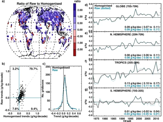
Figure 5a to c show trends in the data before and af-ter homogenisation. There is generally good agreement with 87.2 % of grid boxes being of the same sign (drying or moist-ening) in both the raw and homogenised data (Fig. 5a and b). However, it is clear that the raw data show trends of a slightly greater magnitude (both wetter and dryer) than the homogenised data (Fig. 5c). In terms of the large-scale average, homogenisation appears to have very little effect (Fig. 5d–g). The trend for the Northern Hemisphere is very slightly smaller after homogenisation, and the trend in the Southern Hemisphere is slightly larger. The largest differ-ences in the time series occur for the tropics and South-ern Hemisphere. This is likely an artefact of the low spatial coverage here compared to the extratropical and midlatitude Northern Hemisphere, where averaging over many stations can moderate the effect of changes to a few stations. Fur-thermore, the tropics include some of the largest magnitude adjustments. The fact that changes are very small on these large scales suggests that seasonal analyses on large scales (not presented here) may be reasonable despite the lack of seasonally varying homogenisation. However, we urge care when analysing over smaller regions, individual grid boxes and stations, where any remaining inhomogeneity or unde-sirable effect of applying flat adjustments may be larger. A set of individual stations representing some of the largest changes in trends before and after homogenisation are dis-played with respect to the surrounding station network in Fig. 6a to c.
There will always be change points (both step changes and local trends) which remain undetected because they are either too small to detect or too close to other change points. It is very difficult to estimate the uncertainty remaining in the data due to missed detections and adjustments without a rigorous benchmarking exercise as has been undertaken for tempera-ture over the USA (Williams et al., 2012). Benchmarking is a relatively new concept and so has not yet been attempted for humidity, and as such, is beyond the scope of this paper.
4 Estimating an uncertainty model for specific humidity
4.1 Station uncertainty
Our estimate of the monthly mean anomalyqanom is given,
following Brohan et al. (2006), by
qanom=qob−qclim+qadj, (7)
whereqob is the observed monthly mean; qclim is the
Fig. 4.Distribution of adjustments made and their magnitude during the pairwise homogenisation process:(a)adjustments by latitude;
(b)largest adjustments for each station. Note non-linear colour bars.
long-term homogeneity. In fact, there is an error term,ε, in-herent in each of these terms such that the true monthly mean anomaly can be described as
qanom=qob−qclim+qadj+εob+εclim+εadj. (8)
Unfortunately, these errors cannot be quantified explicitly, and so the uncertainty, u, in each monthly mean anomaly value needs to be estimated. To determine the significance ofqanom, we estimate the uncertaintyuanomthat captures the
likely error from each of the error terms in Eq. (8): uanom=
q
u2clim+u2adj+u2ob, (9) whereuclimis the uncertainty in the calculation of the
clima-tological monthly mean due to missing data (temporal sam-pling uncertainty);uadjis the uncertainty in the adjustments applied for homogeneity; and uob is the measurement
un-certainty of meteorological measurements. We now consider each of these in turn.
The standard uncertainty in the climatological monthly mean due to missing data is given by
uclim =√σclim NM
, (10)
whereσclimis the standard deviation of theNMmonths
mak-ing up the climatological mean of the 30-yr period from 1976 to 2005.
The standard uncertainty in the applied homogeneity ad-justments, uadj, is estimated as the quadrature sum of two
terms: uadj=
q
u2applied+u2missed. (11)
The first termuappliedarises from the adjustments whichhave
been applied to the data, and the second termumissedarises
from the adjustments which have not been applied to the data, but which should have been.
We estimateuappliedfrom the 5th to 95th percentile spread
of all possible adjustment magnitudes given by the network of pairwise evaluations, as described in Sect. 3.1, adjusting by a factor 1.65 to obtain a standard uncertainty (1σ, cover-age factor ofk=1).
We estimateumissed, the uncertainty arising from missed
change points, using methods described in Brohan et al. (2006). We assume that large change points, shown in the tails of the distribution in Fig. 3a (black line), are well captured because they are easy to detect given the high signal-to-noise ratio. However, the small adjustments, close to 0 g kg−1, are not well captured, as shown by the “missing middle” of the distribution. The central part of the distribu-tion can be approximated by a Gaussian distribudistribu-tion. A best-fit curve is then derived by merging a best-fitted Gaussian curve (near the centre) with those points of the actual adjustment distribution that are larger (in the wings). The standard devi-ation of the difference between this “best fit” and the actual distribution (blue dotted line) is 0.135 g kg−1 and provides an estimate ofumissed.
The uncertainty uob relates to the uncertainty of
mea-surement of the instrument at the point of observation. The
BIPMGuide to the Expression of Uncertainty in
Ratio of Raw to Homogenised
-2.00 -1.00 -0.50 0.00 0.50 1.00 2.00 ratio
a)
-0.5 0.0 0.5 1.0 Homogenised trends (g/kg/decade)
-0.5 0.0 0.5 1.0
Raw trends (g/kg/decade)
79.7%
9.4% 7.6%
3.2%
b)
-0.4 -0.2 0.0 0.2 0.4 0.6 Trend (g/kg/decade) 0
50 100 150 200 250
No. gridboxes
Homogenised
Raw
c)
-0.6 -0.4 -0.2 -0.0 0.2 0.4 0.6
g/kg
GLOBE (70S-70N)
d) Homogenised
Raw (dotted)
0.09 g/kg/dec ( 0.07 to 0.11)
0.09 g/kg/dec ( 0.06 to 0.11)
-0.6 -0.4 -0.2 -0.0 0.2 0.4 0.6
g/kg
N. HEMISPHERE (20N-70N)
e)
0.08 g/kg/dec ( 0.06 to 0.11)
0.08 g/kg/dec ( 0.06 to 0.10)
-0.6 -0.4 -0.2 -0.0 0.2 0.4 0.6
g/kg
TROPICS (20S-20N)
f)
0.13 g/kg/dec ( 0.10 to 0.17)
0.14 g/kg/dec ( 0.11 to 0.19)
-0.6 -0.4 -0.2 -0.0 0.2 0.4 0.6
g/kg
1975 1980 1985 1990 1995 2000 2005 2010 YEAR
S. HEMISPHERE (70S-20S)
g)
0.01 g/kg/dec (-0.02 to 0.04)
-0.03 g/kg/dec (-0.05 to 0.01)
Fig. 5.Difference between trends (1973–2012) in HadISDH before and after the pairwise homogenisation process.(a)Ratio of decadal trends from the raw HadISDH compared to homogenised HadISDH (trend methodology is described in Fig. 9). Note non-linear colour bars.
(b)Scatter relationship between homogenised and raw decadal trends for HadISDH. The percentage of grid boxes present in each quadrant is shown.(c)Distribution of grid-box trends for the homogenised and raw data.(d–g)Large-scale area average annual anomaly time series and trends for homogenised HadISDH and the raw data relative to the 1976–2005 climatology period.
knowledge of the measurement apparatus and the measuring conditions. Type B uncertainties may have randomly vary-ing components,urand, and components which cause
“sys-tematic” errors,usys.
In a meteorological context it is not possible to derive Type A estimates of uncertainty because the measurand – the weather – is intrinsically variable, and so the variability due to the instruments themselves cannot be isolated. Since Type A uncertainties are likely to be random and uncorre-lated, they should reduce with temporal and spatial averag-ing to a large extent, and so be attenuated by averagaverag-ing both over a month and over a grid box. Since the station meta-data do not reliably record the instrumentation used, we have derived estimates of the Type B uncertainty of an individual measurementui based on knowledge of hygrometers in use
in the field. Until the 1980s, psychrometers were probably the most common type of hygrometer, but since then there has been a move towards electronic devices (typically capac-itance sensors) and dewcels which can be more readily auto-mated. Typically, electronic devices have a lower uncertainty than psychrometers, and so we can conservatively estimate ui(Table 2) assuming that all humidity measurements were
taken using aspirated psychrometers.
Psychrometer errors arise either from the use of an incor-rect psychrometer coefficient, or from temperature errors in measurements of either the wet bulb or dry bulb (MOHMI, 1981). In general, these errors are not random or symmetri-cally distributed, and they may be correlated with other me-teorological variables, such as wind speed. However, we ex-pect that within any one month, the uncertainty of measure-ment for psychrometers will contain some random compo-nent,urand, whose effect can be reduced by averaging, and a systematic component,usys, whose effect will be unaffected
by averaging.
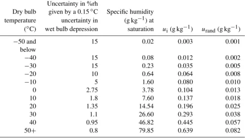
We estimate ui with a standard uncertainty of 0.15◦C
Fig. 6.Results for three stations as examples of some of the largest changes of the pairwise homogenisation algorithm. Red lines represent the original station time series. Blue lines represent the adjusted time series. Black lines show the original time series for all stations within the designated network.(a)Sur, Oman, WMO ID: 412680, 22.533◦N, 59.467◦E, 14.0 m.(b)Atar, Mauritania, WMO ID: 614210, 20.5170◦N, 13.0670◦W, 224.0 m.(c)Sao Luiz, Brazil, WMO ID: 822810, 2.6000◦S, 44.2330◦W, 53.0 m.
Table 2.Estimates of standard uncertainty in humidity measurements calculated in terms of equivalent psychrometer uncertainty to represent a “worst case scenario”. At lower temperatures the measurement uncertainty becomes large, but the low absolute specific humidity values make only a small contribution to global estimates of specific humidity. Calculations of specific humidity used Eqs. (1) to (5).
Uncertainty in %rh
Dry bulb given by a 0.15◦C Specific humidity temperature uncertainty in (g kg−1) at
(◦C) wet bulb depression saturation ui(g kg−1) urand(g kg−1)
−50 and 15 0.02 0.003 0.001
below
−40 15 0.08 0.012 0.002
−30 15 0.23 0.035 0.005
−20 10 0.64 0.064 0.008
−10 5 1.60 0.080 0.010
0 2.75 3.78 0.104 0.013
10 1.8 7.60 0.137 0.018
20 1.35 14.54 0.196 0.025
30 1.1 26.60 0.293 0.038
40 0.95 46.82 0.445 0.057
50+ 0.8 79.85 0.639 0.082
vapour pressure calculated from simultaneous monthly mean T (Eqs. 1 and 2), under the necessary (and in many cases in-correct) assumption that theT data are homogeneous, the re-sulting change inqcan be estimated. The reading uncertain-ties of the wet bulb and dry bulb temperatures are unlikely to be biased, and so we assume that the resulting uncertainty is randomly distributed. We thus estimate the random compo-nent of the uncertainty in the monthly mean as
urand=
ui √
NO
. (12)
In order to pass ISD quality control, there must be at least 15 days of data for a monthly mean and at least four observa-tions per day, implyingNO≥60. Hence, we conservatively
useNO=60 in our calculation ofurand.
There are a number of weaknesses in this approach. Firstly, these non-linear conversions (Eqs. 1 to 5) are im-perfect for monthly mean data. Secondly, when the monthly
value is already close to 100 %rh, the addition of uncertainty in RH can then result in estimates >100 %rh. Although it is physically possible for RH to exceed 100 %rh, it is not common, nor reliably measured in operational circumstances (Makkonen and Laakso, 2005). Thirdly, errors will also be introduced because the simultaneous monthly meanT data have not been homogenised. This is due to the issue of main-taining physical continuity when homogenising across si-multaneously observed variables which will be addressed in future work. False wet bulb depressions may occur at 100 %rh, but the low-resolution conversion between humid-ity variables makes accurate detection of such cases impos-sible. However, limiting the new RH (%rh + derived uncer-tainty in %rh) to 100 %rh can imply an unrealistically small variability. To counter this, we have set a minimum thresh-old forurand of two standard deviations below the mean by
All values below this threshold are assumed to be unrealisti-cally low and are substituted with the mean value ofurandfor that station.
Despite the difficulties in estimatingurand, one clear
fea-ture emerges (Table 2). Although the fractional uncertainties are largest at low temperatures, the absolute values of specific humidity are low in this range – saturation vapour pressure varies by a factor 20 from 0◦C to 50◦C – and so contribu-tions to the uncertainty in the specific humidity of a station will be dominated by the uncertainty during periods of high temperature and high relative humidity.
In addition to randomly varying components,ui, the
uncer-tainty of measurement of each station, will also have contri-butions which do not reduce on averaging,usys. Such
uncer-tainties arise from the limitations of the calibration, and the shortcomings of psychrometers. We have not included an ex-plicit assessment ofusysbecause we consider that their effect on our estimate ofqanom is likely to be small. The origin of
this insensitivity can be seen by considering the case in which a change point is identified as occurring in the record from a particular station, and also the case in which no change points are identified. For example, where instruments or observing practices change or stations move,usys will change, and so
we expect that some fraction ofusys should be found
dur-ing homogenisation and so should be partially accounted for in terms ofuadj. Additionally, when a change point is found
by comparison with neighbouring stations, the algorithm ad-justs the target station’s older data to match its newer data on the assumption that more modern measurements are likely to have lower uncertainty. Where instruments or observing practices donotchange, then we can assume thatusyswill be substantially unchanged. So we expect that a substantial fraction ofusys will be common to qanom and qclim. Thus,
when calculatingqanomwe can expect this fraction of the
un-certainty to cancel (Eq. 8). However, we note that care must be taken if the final gridded data are used to estimate abso-lutevalues of specific humidity. For such cases, the full value ofusysshould be evaluated to fully capture the uncertainty.
The uncertainty estimates provided alongside HadISDH will therefore be underestimates with respect to theabsolute val-ues.
The uncertainties are calculated as standard uncertainties (1σ ), and then a coverage factork=2 is applied such that there is∼95 % confidence (2σ )that these uncertainties cap-ture the true error. As an example, the individual uncertainty components and the combined station uncertainty are shown in Fig. 7 for station 486650 (Malacca, Malaysia, 2.267◦N, 102.250◦E, 9.0 m). Climatological uncertainty is constant year to year, but has an annual cycle and is greatest during the season of greatest natural variability inq. Measurement un-certainty (not includingusys)is usually the smallest
compo-nent. It changes throughout but has a clear annual cycle due to the temperature dependence. The adjustment uncertainty is usually the largest component, reducing towards 0 g kg−1 because the most recent period is treated as the reference
48665099999 Monthly Anomalies (homogenised)
-2 -1 0 1
g/kg
1975 1980 1985 1990 1995 2000 2005 2010
Monthly Adjustments
-0.3 -0.2 -0.1 0.0
g/kg
1975 1980 1985 1990 1995 2000 2005 2010
Monthly Adjustment Uncertainty
0.0 0.1 0.2 0.3 0.4 0.5 0.6
g/kg
1975 1980 1985 1990 1995 2000 2005 2010
Monthly Observation Uncertainty
0.00 0.02 0.04 0.06 0.08 0.10
g/kg
1975 1980 1985 1990 1995 2000 2005 2010
Monthly Climatology Uncertainty
0.00 0.05 0.10 0.15 0.20 0.25 0.30
g/kg
1975 1980 1985 1990 1995 2000 2005 2010
Monthly Station Uncertainty
0.0 0.1 0.2 0.3 0.4 0.5 0.6
g/kg
1975 1980 1985 1990 1995 2000 2005 2010
Fig. 7.The components of station uncertainty estimates for station 486650 (Malacca, Malaysia, 2.267◦N, 102.250◦E, 9.0 m). All un-certainties represent 2σ(approximately 95 % confidence intervals).
period. This is the first attempt at quantifying uncertainty in specific humidity and is a basis which will benefit from fu-ture improvements in the model design and application as a greater understanding of this issue accrues.
4.2 Gridding methodology and sampling uncertainty
HadISDH is intended for the purpose of studying change on large temporal and spatial scales, so gridding is essential. It reduces the effect of individual outliers and remaining ran-dom errors in the data. Given that station density is rather sparse over large parts of the globe, there is little value in gridding at finer than 5◦ by 5◦ resolution. For the station-rich regions, specific high-resolution grids could be produced but will not be presented here. Using 5◦by 5◦grids also al-lows comparison with other products such as HadCRUH and CRUTEM4.
over the reference period. The standard deviation of all con-tributing stations is also given for each grid-box month, pro-viding an estimate of grid-box variability. Where only one station contributes, an arbitrarily large standard deviation of 100 is given so that these can be easily identified. Station numbers for each grid-box month are also recorded.
Station uncertainty estimates, as defined in Section 3.3, are also brought through to the grid-box level by assuming in-dependence of, and combining in quadrature, all constituent station uncertainties and then multiplying by 1/√(NS),
whereNS is the number of stations in the grid box at that
time. Figure 8a shows an example field of gridded station uncertainty for June 1980 in g kg−1. Station uncertainty is largest around the tropics, whereas for the CRUTEM3 tem-perature product in Brohan et al. (2006) it is largest at the poles. The largest component is by far the adjustment un-certainty, until the most recent years of the record where it tends towards zero as a result of choosing the most recent period as the reference period. The measurement uncertainty is comparable to the climatological uncertainty when aver-aged over the grid-box scale. All are generally largest in the tropics, where station density is generally least. These uncer-tainties are also gridded individually.
Given that there are relatively small numbers of stations within each grid box, the grid-box value is unlikely to be the true grid-box average. Some estimate of the sampling uncer-tainty is necessary. Following Brohan et al. (2006), the sam-pling uncertainty is estimated using the method laid out in Jones et al. (1997). For grid boxes with data we first estimate the mean variance of individual stations in the grid box,s2i, using
s2i = Sˆ
2N SC
(1+(NSC−1)r)
, (13)
whereSˆ2 is the variance of the grid-box anomalies calcu-lated over the 1976–2005 climatology period andNSCis the
mean number of stations contributing to the grid-box mean. The last term,r, is the average inter-site correlation and is estimated using
r=x0 X
1−exp−x0 X
, (14)
whereX is the diagonal distance across the grid box andx0
is the correlation decay length between grid-box averages. Grid-box sampling uncertainty, SE2, is then estimated by
SE2= (s
2
ir(1−r))
(1+(NS−1)r)
. (15)
However, hereNSis the actual number of stations
contribut-ing to the grid box in each month, givcontribut-ing a time varycontribut-ing SE2.
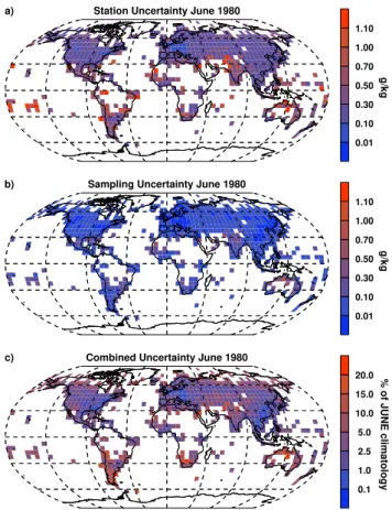
The number of stations contributing to the grid-box mean makes a large difference to SE2, with a 10-fold increase in stations making SE2 an order of magnitude smaller. Sam-pling uncertainties, in g kg−1, are shown in Fig. 8b as 2σ
Station Uncertainty June 1980 a)
0.01 0.10 0.30 0.50 0.70 1.00 1.10
g/kg
Sampling Uncertainty June 1980 b)
0.01 0.10 0.30 0.50 0.70 1.00 1.10
g/kg
Combined Uncertainty June 1980 c)
0.1 1.0 2.5 5.0 10.0 15.0 20.0 % of JUNE climatology
Fig. 8.Examples of gridded 2σ uncertainty fields for HadISDH in June 1980 for(a)station uncertainty,(b)sampling uncertainty and
(c)combined uncertainty as a percentage of the grid-box climato-logical (1976–2005) value for June. Note non-linear colour bars.
uncertainties. The main driver of the sampling uncertainty is the standard deviation of grid-box monthly specific humidity anomalies.
The sampling uncertainty and station uncertainty esti-mates are assumed to be independent and are combined in quadrature to provide a combined uncertainty statistic, shown for June 1980 in Fig. 8c as a percentage of June clima-tology. Station uncertainty is the largest component and dom-inates the combined uncertainty fields where there are data. The magnitude of the combined uncertainty relative to clima-tology is generally less than 5 % (for 69.3 % of grid boxes) but exceeds 10 % of June climatology in 8.0 % of grid boxes, which are mostly located in parts of the subtropics. This re-flects the large uncertainty in adjustments made to the data. For there to be confidence in any changes apparent in the data, these changes must be larger than the combined spread of uncertainty.
by 5◦grid-box scale is small. A recent study by Asokan et al. (2010) found changes in evapotranspiration flux resulting from irrigation over the Mahanadi River Basin in India sug-gesting that local water use could be important in regional climate change. Further work is needed to quantify this im-pact for the global scale.
Another way to explore the uncertainty would be to pro-duce plausible ensemble estimates of HadISDH, as was done for HadCRUT4 (Morice et al., 2012) or Remote Sensing Systems’ Microwave Sounding Units product (Mears et al., 2011). This is the first time that a global humidity esti-mate has been given any measure of uncertainty. Creating a meaningful ensemble product that enables the uncertainty model developed here and its interdependencies through the HadISDH processing chain to be more fully explored is a future aspiration.
4.3 Using the uncertainty model to explore uncertainty
in long-term trends
To explore the uncertainty in individual grid-box trends (Sect. 5.2), a simple 100 member ensemble of HadISDH is created, randomly sampling across the spread of the 2σ un-certainty for each individual unun-certainty component (clima-tology, measurement, adjustment and sampling uncertainty). This is distinct from that described at the end of Sect. 4.2, which would be a far more rigorous exploration of the un-certainty fields. The ensemble members created here while available to users, are purely for exploring the spread of un-certainty and not to be used singularly as a plausible estimate of land surface humidity.
For each station, ten versions of anomaly time series are created by adding the actual anomaly values to random val-ues of climatology, measurement and adjustment errors as follows:
– Climatology error time series: ten values are randomly
selected from a Gaussian distribution (µ=0, 2σ =1) for each station. The Gaussian distribution is forced to have 2σ =1 because this then provides a ∼95 % chance that the randomly selected values lie between −1 and 1. These values are then used as a scaling factor on the 2σ climatology uncertainty which has an annual cycle but is constant year to year.
– Measurement error time series:ten time series are
cre-ated by randomly selecting values from the Gaussian distribution for each station and each month. These are then used as scaling factors on the 2σmeasurement un-certainty, such that the error randomly varies over time.
– Adjustment error time series:ten time series are created
by randomly selecting values from the Gaussian distri-bution for each station and each homogeneous subpe-riod (the pesubpe-riod between two adjustments). These are then used as scaling factors on the adjustment uncer-tainty for each homogeneous subperiod.
For each station, the actual anomalies are then added to the first climatology error time series, the first measurement error time series and the first adjustment error time series to give the first station realisation. The second to tenth station realisations are created similarly. These ten realisations of each station are then gridded in the same manner as the ac-tual HadISDH to give ten gridded realisations. For sampling error, ten values are randomly selected from a Gaussian dis-tribution and used as scaling factors on the sampling uncer-tainty. The scaling factor is consistent across all grid boxes and months within each of the ten sampling error realisations. These are then combined with each of the ten gridded station realisations to give the 100 member ensemble of the gridded HadISDH.
To explore the uncertainty over large-area averages (Sects. 5.3 and 5.4), the spatial coverage uncertainty is es-timated and combined with the station and sampling uncer-tainties, after Brohan et al. (2006), for the globe, Northern Hemisphere, tropics and Southern Hemisphere. As the spa-tial coverage of the gridded data is not globally complete and varies from month to month, this uncertainty needs to be accounted for when creating a regional average time se-ries. To estimate the uncertainties of these large-area aver-ages, which are based on incomplete coverage, we use the ERA-Interim reanalysis product due to its good agreement with the in situ surface humidity (Simmons et al., 2010). For each month in the HadISDHq anomalies, the ERA-Interim qanomalies from all matching calendar months are selected (i.e. for a January in HadISDH, all Januaries in ERA-Interim are selected). The ERA-Interim fields are then masked by the spatial coverage in HadISDH for that particular month and a cosine-weighted regional average is calculated. The resid-uals between these masked averages and the full regional average are then calculated. From the distribution of these residuals, the standard deviation is extracted and used as the spatial coverage uncertainty for that HadISDH month in the regional time series. The sampling and station uncertainties are estimated from the individual sampling and station uncer-tainties for each grid box, and then combined with the overall coverage uncertainty for the region in question. On a month-by-month basis, the sampling and station uncertainties from each grid box are treated as independent errors, and so the re-gional sampling and station uncertainty is the square root of the sum of the normalised cosine-weighted squares of the in-dividual grid-box uncertainties. Inin-dividual components (sta-tion, grid-box sampling and spatial coverage) are also treated as independent, and so root-sum-squared as appropriate to obtain the final 2σ uncertainty on the area-average time se-ries.
uncertainties, normalised by 12 to account for the number of months. The station uncertainty, however is treated as completely autocorrelated, and so the annual station uncer-tainty is the mean of all 12 monthly uncertainties. For the annual coverage uncertainty, the comparison between ERA-Interim and HadISDHq fields is repeated for annual aver-ages (as for monthly). The three individual components are then combined as described above. We note that the treat-ment of the station uncertainty as completely autocorrelated, and the sampling uncertainty as completely uncorrelated, is an approximation, as these uncertainty components are them-selves combinations of separate estimates of the uncertainty from different sources. The climatology component (Eqs. 7 to 10) for example, although uncorrelated between months, is correlated across years (i.e. January to February is uncorre-lated, but January in year 1 to January in year 2 is correlated).
5 Recent trends in land surface specific humidity
5.1 Validation against other land surface
humidity products
It is first necessary to assess the likely quality of HadISDH before we can use it with any confidence. This has been done by comparing grid-box decadal trends with the older Had-CRUH product (Fig. 9) and large-scale area average time se-ries with all other existing products: HadCRUH (Willett et al., 2008); HadCRUHext (Simmons et al., 2010); Dai (Dai, 2006); and the reanalysis product ERA-Interim (from 1979 onwards) regridded to 5◦by 5◦and weighted by percentage of land within each grid box (Dee et al., 2011; Willett et al., 2011, 2012) (Fig. 10a to d). The ERA-Interim time series are shown both spatially matched to HadISDH and with com-plete land coverage.
In all cases trends have been estimated using the median of pairwise slopes (Sen, 1968; Lanzante, 1996). Confidence in the trend is assigned using the 95 % confidence range in the median value. Where the intervals defined by the confidence limits are either both above zero or both below zero, there is high confidence that the trend is significantly different from a zero trend. The spread of these intervals gives an estimate of confidence in the magnitude of the trends.
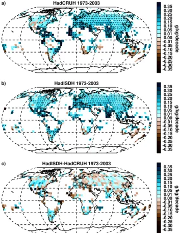
For the grid-box trends over the common period 1973– 2003, HadISDH shows generally good agreement with Had-CRUH – the key feature of widespread moistening is com-mon to both with drying apparent in parts of southern Africa, southern South America, southern Australia and New Zealand. HadCRUH shows more moistening in the tropics (e.g. Brazil, western Africa and northern India). HadISDH shows more moistening over the USA and south-east Asia. There is very little overall difference, with 92.3 % of HadISDH grid boxes showing moistening versus 89.5 % in HadCRUH. It is likely that HadISDH contains fewer out-lying/poor quality data issues due to the improved quality
HadCRUH 1973-2003 a)
-0.35 -0.30 -0.25 -0.20 -0.15 -0.10 -0.05 -0.01 0.00 0.01 0.05 0.10 0.15 0.20 0.25 0.30 0.35
g/kg/decade
HadISDH 1973-2003 b)
-0.35 -0.30 -0.25 -0.20 -0.15 -0.10 -0.05 -0.01 0.00 0.01 0.05 0.10 0.15 0.20 0.25 0.30 0.35
g/kg/decade
HadISDH-HadCRUH 1973-2003 c)
-0.35 -0.30 -0.25 -0.20 -0.15 -0.10 -0.05 -0.01 0.00 0.01 0.05 0.10 0.15 0.20 0.25 0.30 0.35
g/kg/decade
Fig. 9.Decadal trends in specific humidity for HadCRUH versus HadISDH over the 1973–2003 period of record. Trends have been estimated using the median of pairwise slopes (Sen, 1968; Lan-zante, 1996) method. Where intervals defined by the 95 % confi-dence limits on the median of the slopes are both of the same sign as the median trend presented in the grid boxes, the trend is pre-sumed to be significantly different from a zero trend. This is indi-cated by a black dot within the grid box. This means that there is higher confidence in the direction of the trend, but not necessar-ily the magnitude. The spread of the confidence interval provides the confidence in the magnitude; these values are available online at www.metoffice.gov.uk/hadobs/hadisdh. Note non-linear colour bars.
control and homogenisation methods used. There are large differences over the USA owing to the improvements in cov-erage and station compositing described in Sect. 2; see also Smith et al. (2011). In HadISDH, moistening is now far more widespread over the USA.
Fig. 10.Time series of large-scale average specific humidity over land for HadISDH and existing data products.(a–d)Annual time series from all other global surface humidity products given a zero mean over the common period of 1979–2003. Dai covers 60◦S to 70◦N. ERA-Interim has been weighted by % land coverage in each grid box and is shown both spatially matched to HadISDH and with complete coverage.(e–h)Monthly time series (relative to the 1976–2005 climatology period) for HadISDH with 2σuncertainty estimates. The black line is the area average (using weightings from the cosine of the latitude). The red, blue and orange lines show the±combined uncertainty estimates from the grid-box sampling uncertainty, the station uncertainty and the spatial coverage uncertainty, respectively. Decadal trends are shown for each region for the period 1973–2012. These have been fitted to the monthly-mean anomaly time series using the median of pairwise slopes as described in Fig. 9, with the 95 % confidence intervals shown. Where these are both of the same sign (i.e. the globe, Northern Hemisphere and tropics) there is high confidence that trends are significantly different from zero.
Simmons et al. (2010), a change in SST source ingested into ERA-Interim in 2001 led to a cooler period of SSTs hence-forth, which almost certainly led to slightly lower surface specific humidity from 2001 onwards, even over the land. This is apparent in Fig. 10a to d. While Dai, HadISDH and all varieties of HadCRUH use the same source data, the methods are independent and station selection differs. ERA-Interim does ingest surface humidity data indirectly through its use for soil moisture adjustment, but also has strong constraints from the 4D-Var atmospheric model and many other data products, so it can be considered independent (Simmons et al., 2010). However, it is not impossible that the ERA-Interim reanalysis and the in situ products may be jointly affected by a contiguous region of poor station quality.
Users should note that annual updates to HadISDH will likely also involve some changes to the historical record as the ISD source database is undergoing continual improve-ments to its historical archives. This can result in the addi-tion of some staaddi-tions into HadISDH that will then have suffi-ciently long data series. It may also result in the loss of some
stations where ISD updates have resulted in their removal or merges with another record. There may be loss or addi-tion of years of data for staaddi-tions that remain in HadISDH. In some cases this may change the underlying station trends. While using grid-box average anomalies mitigates the ef-fects of this instability somewhat, some notable differences could persist through to the grid-box level. Changes are un-likely to affect the large-scale features of the data. In updat-ing from 2011 to 2012, the HadISDH trend for large-scale av-erage changed minimally (±0.01 g kg−1per decade). Com-parisons will be made after each update and documented at www.metoffice.gov.uk/hadobs/hadisdh/.
5.2 Spatial patterns in long-term changes in land
surface specific humidity
-0.35 -0.30 -0.25 -0.20 -0.15 -0.10 -0.05 -0.01 0.00 0.01 0.05 0.10 0.15 0.20 0.25 0.30 0.35 g/kg/decade
Fig. 11.Decadal trends in specific humidity for HadISDH over 1973–2012. Trends are fitted and confidence assigned as described in Fig. 9. Note non-linear colour bars.
extensive drying in parts of South America and western and eastern USA, and Mexico; and south-ern Africa showing more moistening. Overall, there is widespread moistening which is strongest across the trop-ics. The subtropics over the USA, South America and Aus-tralia show drying. This is consistent with the now well-observed and documented intensification of the hydrological cycle over recent decades (Allan et al., 2010).
The grid-box trends range from approximately −0.1 g kg−1 to 0.3 g kg−1 per decade. This is compara-ble to the uncertainty ranges shown in Fig. 8. To explore the uncertainty in these trends, an ensemble of HadISDH is created with 100 members as described in Sect. 4.3. Trends are fitted to each ensemble member at the grid-box scale. The 5th percentile, median and 95th percentile trends for each grid box (assessed individually) are shown in Fig. 12 a to c, respectively. Moistening remains the main feature of all three maps, so the conclusion of widespread moistening appears to be robust to the quantified uncertainties, espe-cially across the tropics, Eurasia and north-eastern North America. Drying over the south-western USA also appears to be significant relative to uncertainty, but the extratropical drying regions show relatively large uncertainty.
5.3 Long-term changes in large-scale area average land
surface specific humidity
For the globe, Northern Hemisphere and tropics, the un-certainty range is smaller than the overall long-term trend (Fig. 10e to h). Hence, we can be confident in the long-term moistening signal shown in the data over these regions. The uncertainty is dominated by the spatial coverage, but the sta-tion and sampling uncertainty will be more important for
5th Percentile a)
-0.35 -0.30 -0.25 -0.20 -0.15 -0.10 -0.05 -0.01 0.00 0.01 0.05 0.10 0.15 0.20 0.25 0.30 0.35
g/kg/decade
Median b)
-0.35 -0.30 -0.25 -0.20 -0.15 -0.10 -0.05 -0.01 0.00 0.01 0.05 0.10 0.15 0.20 0.25 0.30 0.35
g/kg/decade
95th Percentile c)
-0.35 -0.30 -0.25 -0.20 -0.15 -0.10 -0.05 -0.01 0.00 0.01 0.05 0.10 0.15 0.20 0.25 0.30 0.35
g/kg/decade
Fig. 12.Exploration of the uncertainty in decadal trends using 100 realisations of HadISDH spread across the 2σ uncertainty esti-mates. Median pairwise trends were fitted over the period for each realisation, with higher confidence assigned by a black dot as de-scribed in Fig. 9. For each grid box, the 5th percentile(a), median
(b)and 95th percentile(c)trends are shown. If the uncertainty was large enough to obscure the long-term trends, then it would be ex-pected that the 5th and 95th percentiles would starkly disagree with each other. In fact, there is very little difference as shown by(a),
(b)and(c)above. Note non-linear colour-bars.