An integrated assessment modelling framework for uncertainty studies in global and regional climate change: the MIT IGSM-CAM (version 1.0)

(1)

GMDD

6, 2213–2248, 2013

Modelling framework for regional climate change uncertainty

E. Monier et al.

Title Page

Abstract Introduction

Conclusions References

Tables Figures

◭ ◮

Back Close

Full Screen / Esc

Printer-friendly Version Interactive Discussion

Discussion

P

a

per

|

Dis

cussion

P

a

per

|

Discussion

P

a

per

|

Discussio

n

P

a

per

|

Geosci. Model Dev. Discuss., 6, 2213–2248, 2013 www.geosci-model-dev-discuss.net/6/2213/2013/ doi:10.5194/gmdd-6-2213-2013

Geoscientiic Geoscientiic

Geoscientiic

Open Access

Geoscientiic Model Development

Discussions

This discussion paper is/has been under review for the journal Geoscientific Model Development (GMD). Please refer to the corresponding final paper in GMD if available.

An integrated assessment modelling

framework for uncertainty studies in

global and regional climate change:

the MIT IGSM-CAM (version 1.0)

E. Monier1, J. R. Scott1, A. P. Sokolov1, C. E. Forest2, and C. A. Schlosser1

1

Joint Program on the Science and Policy of Global Change, Massachusetts Institute of Technology, Cambridge, Massachusetts, USA

2

Department of Meteorology, Earth and Environmental Systems Institute, Pennsylvania State University, University Park, Pennsylvania, USA

Received: 13 February 2013 – Accepted: 21 March 2013 – Published: 28 March 2013

Correspondence to: E. Monier (emonier@mit.edu)

(2)

GMDD

6, 2213–2248, 2013

E. Monier et al.

Title Page

Tables Figures

◭ ◮

Back Close

Full Screen / Esc

Discussion

P

a

per

|

Dis

cussion

P

a

per

|

Discussion

P

a

per

|

Discussio

n

P

a

per

|

Abstract

This paper describes an integrated assessment modelling framework for uncertainty studies in global and regional climate change. In this framework, the Massachusetts Institute of Technology (MIT) Integrated Global System Model (IGSM), an integrated assessment model that couples an earth system model of intermediate complexity to

5

a human activity model, is linked to the National Center for Atmospheric Research (NCAR) Community Atmosphere Model (CAM). Since the MIT IGSM-CAM framework (version 1.0) incorporates a human activity model, it is possible to analyse uncertain-ties in emissions resulting from both uncertainuncertain-ties in the economic model parameters and uncertainty in future climate policies. Another major feature is the flexibility to vary

10

key climate parameters controlling the climate system response: climate sensitivity, net aerosol forcing and ocean heat uptake rate. Thus, the IGSM-CAM is a

computation-ally efficient framework to explore the uncertainty in future global and regional climate

change associated with uncertainty in the climate response and projected emissions. This study presents 21st century simulations based on two emissions scenarios

(un-15

constrained scenario and stabilization scenario at 660 ppm CO2-equivalent) and three

sets of climate parameters. The chosen climate parameters provide a good approxi-mation for the median, and the 5th and 95th percentiles of the probability distribution of 21st century global climate change. As such, this study presents new estimates of the

90 % probability interval of regional climate change for di_fferent emissions scenarios.

20

These results underscore the large uncertainty in regional climate change resulting from uncertainty in climate parameters and emissions, especially when it comes to changes in precipitation.

1 Introduction

For many years, the Massachusetts Institute of Technology (MIT) Joint Program on the

25

Science and Policy of Global Change has devoted a large effort to estimating

(3)

GMDD

6, 2213–2248, 2013

E. Monier et al.

Title Page

Tables Figures

◭ ◮

Back Close

Full Screen / Esc

Discussion

P

a

per

|

Dis

cussion

P

a

per

|

Discussion

P

a

per

|

Discussio

n

P

a

per

|

the climate response (Reilly et al., 2001; Forest et al., 2008). Based on these PDFs, probabilistic forecasts of the 21st century climate have been performed to inform po-licy makers and the climate community at large (Sokolov et al., 2009; Webster et al.,

2012). This effort has been organized around the MIT Integrated Global System Model

(IGSM), an integrated assessment model that couples an earth-system model of

inter-5

mediate complexity to a human activity model. The IGSM framework presents major advantages in the application of climate change studies. A fundamental feature of the IGSM is the ability to vary key parameters controlling the climate system response to changes in greenhouse gas and aerosol concentrations, e.g. the climate sensitivity, the strength of aerosol forcing and the rate of heat uptake by the ocean (Raper et al., 2002;

10

Forest et al., 2008). As such, the IGSM enables structural uncertainties to be treated

as parametric ones and provides a flexible framework to analyse the effect of some of

the structural uncertainties present in Atmosphere-Ocean Coupled General Circulation Models (AOGCMs). Another major advantage of the IGSM is the coupling of the earth system with a detailed economic model. This allows not only simulations of future

cli-15

mate change for various emissions scenarios to be carried out but also for the analysis of the uncertainties in emissions that result from uncertainties intrinsic to the economic model (Webster et al., 2012).

Since the IGSM has a two-dimensional zonally averaged representation of the at-mosphere, it has been used primarily for climate change studies from a global mean

20

perspective. While future changes in the global mean climate are of primary interest,

a large effort must be undertaken to quantify regional climate change. Probabilistic

projections of future regional climate change would prove beneficial to policy makers and impact modeling research groups who investigate climate change and its soci-etal impacts at the regional level, including agriculture productivity, water resources

25

and energy demand (Reilly et al., 2013). The aim of the MIT Joint Program is to

con-tribute to this effort by investigating regional climate change under uncertainty in the

climate response and projected emissions. Two different approaches have been

(4)

GMDD

6, 2213–2248, 2013

E. Monier et al.

Title Page

Tables Figures

◭ ◮

Back Close

Full Screen / Esc

Discussion

P

a

per

|

Dis

cussion

P

a

per

|

Discussion

P

a

per

|

Discussio

n

P

a

per

|

the IGSM zonal mean atmosphere using a pattern scaling method (Schlosser et al., 2013) and linking a three-dimensional atmospheric model to the IGSM. For studies re-quiring three-dimensional atmospheric capabilities, a new capability of the MIT Joint Program modeling framework is presented where the IGSM is linked to the National Center for Atmospheric Research (NCAR) Community Atmosphere Model (CAM). The

5

MIT IGSM-CAM provides an efficient modeling system that can be used to study

un-certainty in climate change at the continental and regional levels.

In this paper, we present a description of the IGSM, including the earth system model of intermediate complexity and the human activity model, and of the newly developed IGSM-CAM framework (see http://globalchange.mit.edu/research/IGSM/download for

10

information on how to obtain the source code). Then, we show results from 21st cen-tury simulations based on two emissions scenarios (unconstrained emissions scenario

and stabilization scenario at 660 ppm CO2-equivalent by 2100) and three sets of

cli-mate parameters. The chosen clicli-mate parameters provide a good approximation for the median, and the 5th and 95th percentiles of the probability distribution of 21st

15

century climate change. Thus, this study presents estimates of the median and 90 %

probability interval of regional climate change for two di_fferent emissions scenarios.

We then compare the range of projections with that of models from the Coupled Model Intercomparison Project Phase 5 (CMIP5) (Taylor et al., 2012).

2 Modeling framework

20

2.1 The MIT IGSM framework

The MIT IGSM version 2.3 (Dutkiewicz et al., 2005; Sokolov et al., 2005) is a fully coupled earth system model of intermediate complexity that allows simulation of criti-cal feedbacks among its various components, including the atmosphere, ocean, land, urban processes and human activities. The atmospheric dynamics and physics

com-25

(5)

GMDD

6, 2213–2248, 2013

E. Monier et al.

Title Page

Tables Figures

◭ ◮

Back Close

Full Screen / Esc

Discussion

P

a

per

|

Dis

cussion

P

a

per

|

Discussion

P

a

per

|

Discussio

n

P

a

per

|

dynamical representation of the atmosphere at 4◦ _{resolution in latitude with eleven}

levels in the vertical. The ocean component includes a three-dimensional dynamical ocean component based on the MIT ocean general circulation model (Marshall et al., 1997) with a thermodynamic sea-ice model and an ocean carbon cycle (Dutkiewicz

et al., 2005, 2009). The ocean model has a realistic bathymetry, and a 2◦

×2.5◦

res-5

olution in the horizontal with twenty-two layers in the vertical, ranging from 10 m at the surface to 500 m thick at depth. Heat and freshwater fluxes are anomaly coupled in order to simulate a realistic ocean state. In order to more realistically capture sur-face wind forcing over the ocean, 6 hr National Centers for Environmental Prediction (NCEP) reanalysis (Kalnay et al., 1996) of surface 10 m wind speeds from 1948–2007

10

is used to formulate wind stress. The data are detrended through analysis of changes in zonal mean over the ocean (by month) across the full 60 yr period; this has little im-pact except over the Southern Ocean, where the trend is quite significant (Thompson and Solomon, 2002). For any given model calendar year, a random calendar year of wind stress data is applied to the ocean. This approach ensures that both short-term

15

“weather” variability and interannual variability are represented in the ocean’s surface

forcing. Different random sampling can be applied to simulate different natural

variabil-ity in the same way as perturbation in initial conditions.

The IGSM2.3 also includes an urban air chemistry model (Mayer et al., 2000) and a detailed global scale zonal-mean chemistry model (Wang et al., 1998) that

consid-20

ers the chemical fate of 33 species including greenhouse gases and aerosols. The terrestrial water, energy and ecosystem processes are represented by a Global Land Systems (GLS) framework (Schlosser et al., 2007) that integrates three existing mod-els: the NCAR Community Land Model (CLM) (Oleson et al., 2004), the Terrestrial Ecosystem Model (TEM) (Melillo et al., 1993) and the Natural Emissions Model (NEM)

25

(6)

GMDD

6, 2213–2248, 2013

E. Monier et al.

Title Page

Tables Figures

◭ ◮

Back Close

Full Screen / Esc

Discussion

P

a

per

|

Dis

cussion

P

a

per

|

Discussion

P

a

per

|

Discussio

n

P

a

per

|

Finally, the human systems component of the IGSM is the MIT Emissions Predictions and Policy Analysis (EPPA) model (Paltsev et al., 2005), which provides projections of world economic development and emissions over 16 global regions along with analysis of proposed emissions control measures. EPPA is a recursive-dynamic multi-regional general equilibrium model of the world economy, which is built on the Global Trade

5

Analysis Project (GTAP) dataset (maintained at Purdue University) of the world eco-nomic activity augmented by data on the emissions of greenhouse gases, aerosols and other relevant species, and details of selected economic sectors. The model projects economic variables (gross domestic product, energy use, sectoral output,

consump-tion, etc.) and emissions of greenhouse gases (CO₂, CH₄, N₂O, HFCs, PFCs and SF₆)

10

and other air pollutants (CO, VOC, NO_x, SO₂, NH₃, black carbon and organic carbon)

from combustion of carbon-based fuels, industrial processes, waste handling and agri-cultural activities.

A major feature of the IGSM is the flexibility to vary key climate parameters control-ling the climate response. The climate sensitivity can be changed by varying the cloud

15

feedback (Sokolov, 2006) while the strength of the aerosol forcing is modified by

adjust-ing the total sulfate aerosol radiative forcadjust-ing e_fficiency. The rate of oceanic heat uptake

can be changed by modifying the value of the diapycnal diffusion coefficient (Dalan

et al., 2005), resulting in multiple versions of the IGSM2.3 with different ocean heat

uptake rate. The IGSM is also computationally e_fficient and thus particularly adapted

20

to conduct sensitivity experiments or to allow for several millennia long simulations. The IGSM has been used to quantify the PDFs of climate parameters using optimal fingerprint diagnostics (Forest et al., 2001, 2008). This is accomplished by comparing observed changes in surface, upper-air, and deep-ocean temperature changes against IGSM simulations of 20th century climate where model parameters are systematically

25

(7)

GMDD

6, 2213–2248, 2013

E. Monier et al.

Title Page

Tables Figures

◭ ◮

Back Close

Full Screen / Esc

Discussion

P

a

per

|

Dis

cussion

P

a

per

|

Discussion

P

a

per

|

Discussio

n

P

a

per

|

2.2 The IGSM-CAM framework

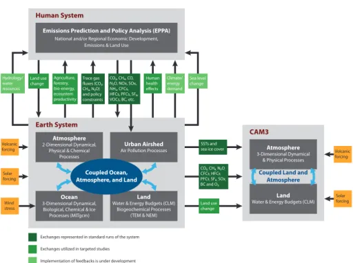
Because the atmospheric component of the IGSM is two-dimensional (zonally avera-ged), regional climate cannot be directly resolved. For investigations requiring three-dimensional atmospheric capabilities, the IGSM is linked CAM version 3 (Collins et al.,

2004), at a 2◦_{x 2.5}◦ _{horizontal resolution with 26 vertical levels. Figure 1 shows the}

5

schematic of the IGSM-CAM (version 1.0) framework. Because CAM3 is coupled to CLM, it provides a representation of the land consistent with the IGSM. For further consistency within the IGSM-CAM framework, new modules were developed and im-plemented in CAM in order to modify its climate parameters to match those of the IGSM. In particular, the climate sensitivity is changed using a cloud radiative

adjust-10

ment method (Sokolov and Monier, 2012). CAM is driven by greenhouse gas con-centrations and aerosol loading simulated by the IGSM model. Since CAM provides a scaling option for carbon aerosols, the default black carbon aerosol loading is scaled to match the global carbon mass in the IGSM. A similar scaling for sulfate aerosols was implemented in CAM and the default sulfate aerosol loading is scaled so that the

15

sulfate aerosol radiative forcing matches that of the IGSM. The ozone concentrations in CAM are a combination of the IGSM zonal-mean distribution of ozone in the tropo-sphere and of stratospheric ozone concentrations derived from the Model for Ozone and Related Chemical Tracers (MOZART). Finally, CAM is driven by IGSM sea surface temperature (SST) anomalies from a control simulation corresponding to pre-industrial

20

forcing added to monthly mean climatology (over the 1870–1880 period) taken from the merged Hadley-OI SST, a surface boundary dataset designed for uncoupled simu-lations with CAM (Hurrell et al., 2008). The IGSM SSTs exhibit regional biases caused by the coupling o the ocean component with a two-dimensional zonal mean atmo-sphere. This bias is present in the seasonal cycle of the ocean state but SST anomalies

25

(8)

GMDD

6, 2213–2248, 2013

E. Monier et al.

Title Page

Tables Figures

◭ ◮

Back Close

Full Screen / Esc

Discussion

P

a

per

|

Dis

cussion

P

a

per

|

Discussion

P

a

per

|

Discussio

n

P

a

per

|

land and ocean biogeochemical cycles are computed within the IGSM, the IGSM-CAM

is more computationally efficient than a fully coupled GCM, like CCSM3. On the other

hand, the IGSM-CAM does not consider potential changes in the spatial distribution of aerosols and ozone. Overall, the IGSM-CAM provides a framework well adapted for uncertainty studies in global and regional climate change since the key parameters that

5

control the climate system response (climate sensitivity, strength of aerosol forcing and ocean heat uptake rate) can be varied consistently within the modeling framework.

3 Description of the simulations

In this study, results from simulations with two emissions scenarios and three sets of climate parameters are presented. For each set of climate parameters and emissions

10

scenarios, a five-member ensemble is run with different initial conditions (through

ran-dom wind sampling in the IGSM and different initial conditions in CAM) in order to

account for the uncertainty in natural variability, resulting in a total of 30 simulations. The results presented in this study are based on the five-member ensemble mean in order to filter out natural variability.

15

3.1 Emissions scenarios

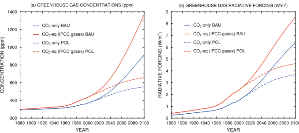
The two emissions scenarios presented in this study are a median unconstrained re-ference scenario where no policy is implemented after 2012, referred to as REF, and

a level 2 stabilization scenario where greenhouse gases are stabilized at 660 ppm CO2

-equivalent (550 ppm CO₂-only) by 2100, referred to as L2S (see Fig. 2). These

emis-20

sions are similar to, respectively, the Representative Concentration Pathways RCP8.5 and RCP4.5 scenarios (Moss et al., 2010). The median unconstrained reference sce-nario corresponds to the median of the distribution obtained by performing Monte Carlo simulations of the EPPA model, using Latin Hypercube sampling of 100 parameters, resulting in a 400-member ensemble simulation (Webster et al., 2008). As opposed

(9)

GMDD

6, 2213–2248, 2013

E. Monier et al.

Title Page

Tables Figures

◭ ◮

Back Close

Full Screen / Esc

Discussion

P

a

per

|

Dis

cussion

P

a

per

|

Discussion

P

a

per

|

Discussio

n

P

a

per

|

to the Special Report on Emissions Scenarios (SRES), this approach allows a more structured development of scenarios that are suitable for uncertainty analysis of an

economic system that results in different emissions profiles. Usually the EPPA scenario

construction starts from a reference scenario under the assumption that no climate poli-cies are imposed. Then additional stabilization scenarios framed as departures from

5

its reference scenario are achieved with specific policy instruments. The 660 ppm CO2

-equivalent stabilization scenario is achieved with a global cap and trade system with emissions trading among all regions beginning in 2015. The path of the emissions over

the whole period (2015–2100) was constrained to simulate cost-effective allocation of

abatement over time. More details on the emissions scenarios in the IGSM can be

10

found in Clarke et al. (2007).

3.2 Climate parameters

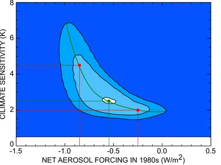
Different versions of the IGSM2.3 exist with different values of the diapycnal diff

u-sion coefficient. The corresponding effective vertical diffusivity is computed using the

methodology described in Sokolov et al. (2003). In this study, we pick the version of

15

the IGSM2.3 with an effective vertical diffusivity of 0.5 cm2s−1_{, which lies between}

the mode and the median of the probability distribution obtained with the IGSM us-ing optimal fus-ingerprint diagnostics (Forest et al., 2008). For this version of the model, the marginal posterior probability density function with uniform prior for the climate

sensitivity-net aerosol forcing (CS-F_ae_{) parameter space is calculated (Fig. 3). We}

20

chose three values of climate sensitivity: the median (2.5◦_{C) and the bounds of the}

90 % probability interval (2.0◦_{C and 4.5}◦_{C). Simulations using the lower, median and}

upper values of climate sensitivities are subsequently referred to as, respectively, lowCS, medCS and highCS. The lower and upper bounds of climate sensitivity agree well with the conclusions of the Fourth Intergovernmental Panel on Climate Change

25

(IPCC) assessment report (AR4) that finds that the climate sensitivity is likely to lie

in the range 2.0–4.5◦_{C (Meehl et al., 2007). Finally, the net aerosol forcing for each}

(10)

GMDD

6, 2213–2248, 2013

E. Monier et al.

Title Page

Tables Figures

◭ ◮

Back Close

Full Screen / Esc

Discussion

P

a

per

|

Dis

cussion

P

a

per

|

Discussion

P

a

per

|

Discussio

n

P

a

per

|

climate change over the 20th century. This is achieved by choosing the net aerosol forc-ing that provides the same transient climate response as the median set of parameters

(see Fig. 3). The values are−0.25 W m−2,−0.55 W m−2 and−0.85 W m−2for,

respec-tively, the lowCS, medCS and highCS simulations. Global climate changes obtained in these simulations provide a good approximation for the median and the 5th and 95th

5

percentiles of the probability distribution of 21st century climate change.

4 Results

4.1 Validation

While CAM has been the subject of extensive validation (Hurrell et al., 2006; Collins et al., 2006b), the IGSM-CAM framework needs to be evaluated for its ability to

simu-10

late the present climate. Figure 4 shows the observed annual-mean merged SST and surface air temperature over land along with the IPCC AR4 multi-model mean error, the typical IPCC AR4 model error and the IGSM-CAM model error, for the median cli-mate sensitivity simulation. IGSM-CAM simulations with low and high clicli-mate sensitivity show very similar results since the associated aerosol forcing was specifically chosen

15

to agree with the observed climate change over the 20th century. While comparing a single model with the IPCC AR4 multi-model mean is useful, it should be noted that in most cases, the multi-model mean is better than all of the individual models (Gleckler et al., 2008; Annan and Hargreaves, 2011). For this reason it is important to consider the typical error as an additional means of comparison and validation of the modeling

20

framework. The IGSM-CAM surface temperature error compares well with the multi-model mean error over most of the globe and is generally within the typical error. The IGSM-CAM surface temperature agrees particularly well with observations over the

ocean, with errors less than 1◦_{C. Over land areas, the IGSM-CAM exhibits regional}

biases, but mainly in areas where the IPCC AR4 typical error is large. For example,

25

(11)

GMDD

6, 2213–2248, 2013

E. Monier et al.

Title Page

Tables Figures

◭ ◮

Back Close

Full Screen / Esc

Discussion

P

a

per

|

Dis

cussion

P

a

per

|

Discussion

P

a

per

|

Discussio

n

P

a

per

|

region and the Hudson Bay, and Eastern Siberia. Meanwhile, a cold bias is present over the coast of Antarctica and the Himalayas. These errors are generally associated with polar regions, where biases in the simulated sea-ice has large impacts on surface temperature, and near topography that is not realistically represented at the resolution of the model. Nonetheless, the IGSM-CAM reproduces reasonably well the end of 20th

5

century surface temperature compared with other available GCMs.

Figure 5 shows a similar analysis for precipitation. The IGSM-CAM is generally able to simulate the major regional characteristics shown in the CMAP annual mean pre-cipitation, including the lower precipitation rates at higher latitudes and the rainbands associated with the Inter-Tropical Convergence Zone (ITCZ) and midlatitude oceanic

10

storm tracks. Nonetheless, the IGSM-CAM model error shows regional biases with pat-terns similar to the mean IPCC AR4 model error, but with larger magnitudes. Like in the IPCC AR4 mean model, the IGSM-CAM precipitation presents a wet bias in the west-ern basin of the Indian Ocean and a dry bias in the eastwest-ern basin. The IGSM-CAM and the IPCC AR4 mean model also show similar biases in precipitation patterns over

15

the Pacific and Atlantic Ocean. The typical IPCC AR4 model error reveals that many of the IPCC AR4 models displays substantial precipitation biases, especially in the trop-ics, which often approach the magnitude of the observed precipitation (Randall et al., 2007). The substantial biases in the simulated present-day precipitation can explain the lack of consensus in the sign of future regional precipitation changes predicted by

20

IPCC AR4 models in parts of the tropics. Compared with the IPCC AR4 models, the skills of the IGSM-CAM framework in simulating present-day annual mean precipitation are reasonably good.

Altogether, Figs. 4 and 5 demonstrate the ability of the IGSM-CAM framework to re-produce present-day surface temperature and precipitation reasonably well compared

25

(12)

GMDD

6, 2213–2248, 2013

E. Monier et al.

Title Page

Tables Figures

◭ ◮

Back Close

Full Screen / Esc

Discussion

P

a

per

|

Dis

cussion

P

a

per

|

Discussion

P

a

per

|

Discussio

n

P

a

per

|

4.2 Global mean projections

Figure 6 shows the changes in global mean surface air temperature and precipitation anomalies from the 1971–2000 period. It shows a broad range of increases in surface temperature by the end of the 21st century, with a global increase between 3.7 and

7.2◦_{C for the reference scenario and between 1.7 and 3.7}◦_{C for the stabilization}

sce-5

nario (based on the 2091–2100 mean anomalies). This is in very good agreement with Sokolov et al. (2009) who performed a 400-member ensemble of climate change sim-ulations with the IGSM version 2.2 for the median unconstrained emissions scenario, with Latin Hypercube sampling of climate parameters based on probability density func-tions estimated by Forest et al. (2008). They found that the 5th and 95th percentiles

10

of the distribution of surface warming for the last decade of the 21st century are

re-spectively 3.8 and 7.0◦_{C when only considering climate uncertainty. This confirms that}

the low and high climate sensitivity simulations presented in this study are representa-tive of, respecrepresenta-tively, the 5th and 95th percentiles of the probability distribution of 21st century climate change. Furthermore, the IGSM-CAM global mean surface air

tem-15

perature anomalies at the end of simulations (year 2100) are in excellent agreement with the IGSM output (shown by the horizontal lines in Fig. 6). This demonstrates the consistency in the global climate response within the framework, largely due to the consistent SST forcing and the matching climate parameters in between the IGSM and CAM. Meanwhile, the changes in global mean precipitation show increases between

20

9.7 and 17.4 mm year−1_{for the reference scenario and between 5.1 and 9.7 mm year}−1

for the stabilization scenario (based on the 2091–2100 mean anomalies). However, it should be noted that even though the IGSM and CAM have very distinct microphysics parameterization schemes, global mean precipitation anomalies in 2100 agree well.

Figure 6 indicates that implementing a 660 ppm CO₂-equivalent stabilization policy can

25

significantly decrease future global warming, with the lower bound warming (from the

1951–2000 mean) below 2◦_{C and the upper bound equal to the lower bound warming}

(13)

GMDD

6, 2213–2248, 2013

E. Monier et al.

Title Page

Tables Figures

◭ ◮

Back Close

Full Screen / Esc

Discussion

P

a

per

|

Dis

cussion

P

a

per

|

Discussion

P

a

per

|

Discussio

n

P

a

per

|

associated with the climate response is of comparable magnitude to the uncertainty associated with the emissions scenarios, thus demonstrating the need to account for both.

4.3 Regional projections

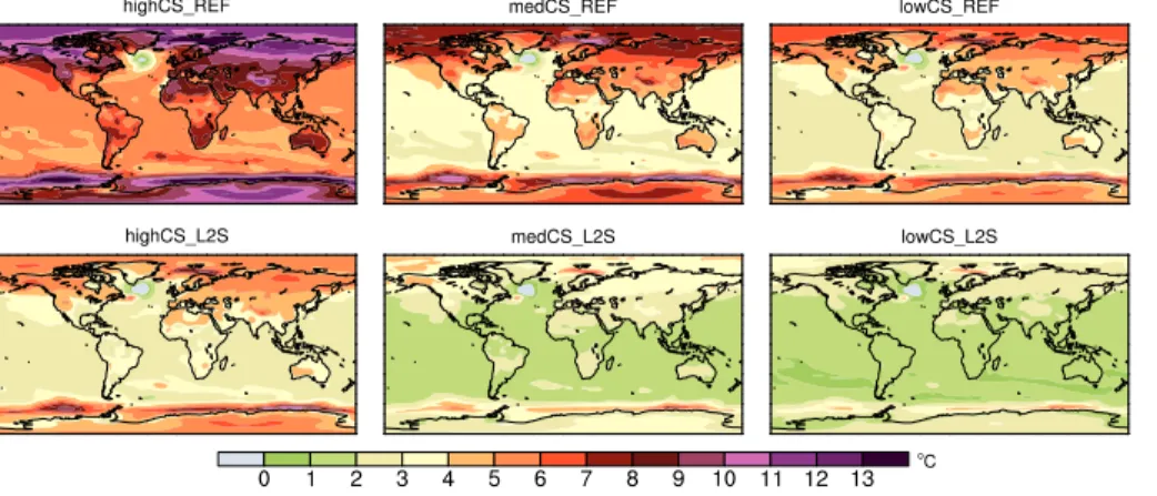
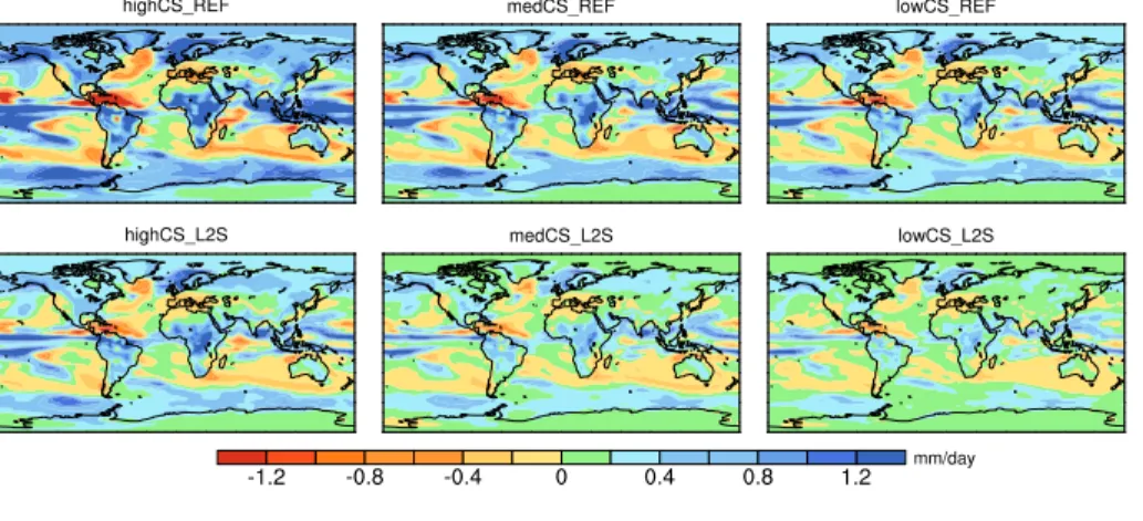
Figure 7 shows maps of the IGSM-CAM ensemble mean changes in annual mean

sur-5

face air temperature between the 1981–2000 and 2081–2100 periods. The analysis of the global mean changes in surface air temperature and precipitation already revealed that the range of uncertainty in the future climate change is large, with similar contri-butions from uncertainty in the climate parameters and in emissions. Figure 7 shows

a wide range of warming between the different scenarios. It also shows well-known

10

patterns of polar amplification and of stronger warming over land. The warming is sig-nificantly weaker over the ocean, except over the coast of Antarctica and over the Arctic Ocean where melting sea-ice leads to a stronger warming. Over high latitude land

ar-eas, the warming ranges between 5 and 12◦_{C for the reference scenario and between}

2 and 6◦_{C for the stabilization scenario. These results indicate that several regions are}

15

at risk of severe climate change, with major potential impacts. For example, the high cli-mate sensitivity simulation for reference scenario shows Northern Eurasia warming by

as much as 12◦_{C in the annual mean and 16}◦_{C in wintertime (not shown). Such}

warm-ing would lead to severe permafrost degradation (Lawrence and Slater, 2005) and the resulting formation of new thaw lakes could lead to enhanced emissions of greenhouse

20

gases, such as methane (Walter et al., 2006). Similarly, Western Europe would warm

by 8◦_{C in the annual mean and 12}◦_{C in summertime. To put this in perspective,}

dur-ing the European summer heat wave of 2003, Europe experienced summer surface air temperature anomalies (based on the June-July-August daily averages) reaching

up to 5.5◦_{C with respect to the 1961–1990 mean (Garcia-Herrera et al., 2010). That}

25

heat wave resulted in more than 70 000 deaths in 16 countries (Robine et al., 2008).

A warming of 12◦_{C in summertime would likely result in serious strain on the most}

(14)

GMDD

6, 2213–2248, 2013

E. Monier et al.

Title Page

Tables Figures

◭ ◮

Back Close

Full Screen / Esc

Discussion

P

a

per

|

Dis

cussion

P

a

per

|

Discussion

P

a

per

|

Discussio

n

P

a

per

|

The same analysis for precipitation is shown in Fig. 8. Precipitation changes show general patterns that are consistent among all simulations. Precipitation tends to in-crease over most of the tropics, at high latitudes and over most land areas. In contrast, the subtropics and midlatitudes experience decreases in precipitation over the ocean. Decreases in precipitation over land are largely restricted to the Western United States,

5

Europe (except Northern Europe), Northwest Africa, Southeast Africa and Patagonia. The magnitude of these patterns of precipitation changes generally increases with in-creasing warming so that the high climate sensitivity simulation for the reference sce-nario presents the largest overall precipitation changes. However, several regions

ex-hibit changes in precipitation of different signs among all the simulations. That is the

10

case of Australia, Southeast China and India. These regions tend to experience de-creases in precipitation for the simulations with the least warming but inde-creases in precipitation with the strongest warming. These results emphasize the fact that only one GCM was used in this study, leading to overall agreement in the regional patterns of precipitation change among all simulations. Nevertheless, there exists regional

un-15

certainty associated with differences in the climate sensitivity (Sokolov and Monier,

2012).

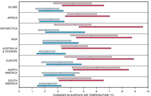
Figure 9 shows the mean and the range of surface air temperature changes over the globe and the seven continents for the period 2081–2100 relative to 1981–2000 for the IGSM-CAM under the reference and level 2 stabilization scenarios and for the

20

CMIP5 models under the RCP8.5 and RCP4.5. The range is estimated for the IGSM-CAM as the minimum and maximum changes over the 30 simulations, while the mean is estimated as the ensemble mean for the median climate sensitivity. The range is estimated for the CMIP5 models as the 90 % range amongst all the models (by re-moving the “outliers”), and the mean is calculated based on all available models at

25

(15)

GMDD

6, 2213–2248, 2013

E. Monier et al.

Title Page

Tables Figures

◭ ◮

Back Close

Full Screen / Esc

Discussion

P

a

per

|

Dis

cussion

P

a

per

|

Discussion

P

a

per

|

Discussio

n

P

a

per

|

be explained by the difference in emissions scenarios, the two scenarios used in this

study having slightly larger radiative forcing than the RCP8.5 and RCP4.5 used by the CMIP5 models. The agreement between the two sets of simulations suggests that the range of warming obtained by the CMIP5 models is likely due to the range of the mod-els’ climate sensitivity, which matches well that of the IGSM distribution. The results

5

also further confirm the wide range of uncertainty in the future global and regional climate change associated with both the uncertainty in emissions and the climate re-sponse. Under the unconstrained emissions scenario, every continent would warm by

at least 2.5◦_{C. The stabilization scenario shows significant reduction in warming over}

all continents. Generally, the upper bound warming under stabilization scenario and

10

the lower bound warming for the reference scenario agree well.

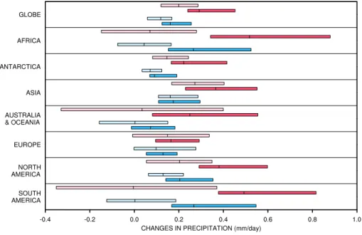
Figure 10 shows the same analysis as Fig. 9 for precipitation. In the IGSM-CAM, all continents experience increases in precipitation, the regional precipitation response is more varied than for temperature. For example, Europe shows little increase in precipi-tation and a narrower range compared with Africa or South America. Europe along with

15

Australia and Oceania show the lower bound of precipitation increase the closest to zero. This is in part due to the choice of regional averaging. Europe and Australia and

Oceania are continents where different regions present opposite signs in the

IGSM-CAM precipitation changes, e.g. Northern Europe shows moistening while the rest of Europe shows drying (see Fig. 8). Finally, Africa and South America show the largest

20

increase in precipitation concurrently with the largest ranges of changes. The agree-ment of the range of precipitation changes between the IGSM-CAM and the CMIP5 models is not as good as for temperature changes. The agreement varies widely

be-tween the different continents. The best agreement is found over Europe and Asia.

Over Australia and Oceania, the IGSM-CAM simulates increases in precipitation while

25

(16)

GMDD

6, 2213–2248, 2013

E. Monier et al.

Title Page

Tables Figures

◭ ◮

Back Close

Full Screen / Esc

Discussion

P

a

per

|

Dis

cussion

P

a

per

|

Discussion

P

a

per

|

Discussio

n

P

a

per

|

disagreement takes place over Africa and South America where the range precipitation changes in the IGSM-CAM does not overlap with the range of the CMIP5 models.

5 Discussion and conclusion

This paper describes a new framework where the MIT IGSM, an integrated assessment model that couples an earth system model of intermediate complexity to a human

activ-5

ity model, is linked to the three-dimensional atmospheric model CAM. The IGSM-CAM

modeling system is an efficient and flexible framework to explore uncertainties in the

future global and regional climate change. First, the IGSM-CAM incorporates a hu-man activity model, thus it can be used to examine uncertainties in emissions resulting from uncertainties intrinsic to the economic model, from parametric uncertainty to

un-10

certainty in future climate policies. Second, the key climate parameters controlling the climate response (climate sensitivity, strength of aerosol forcing and ocean heat uptake rate) can be consistently changed within the modeling framework, so that the IGSM-CAM can be used to address uncertainty in the climate response to future changes in greenhouse gas and aerosols concentrations. Finally, because the atmospheric

chem-15

istry and the land and ocean biogeochemical cycles are computed within the IGSM,

the IGSM-CAM is more computationally efficient than a fully coupled AOGCM.

It should be noted that there are some limitations to the IGSM-CAM framework. First, it is not a fully coupled earth system model. Moreover, the IGSM-CAM frame-work relies on one particular atmospheric model. For this reason, it cannot be used to

20

assess the structural modeling uncertainty arising from differences in the

parameteri-zation suites of climate models. Instead, structural uncertainty has been investigated with the IGSM using a pattern scaling method based on the regional patterns of cli-mate change from the various IPCC AR4 model (Schlosser et al., 2013; Monier et al., 2013). Yet, the IGSM-CAM has advantages over pattern scaling methods, including the

25

(17)

GMDD

6, 2213–2248, 2013

E. Monier et al.

Title Page

Tables Figures

◭ ◮

Back Close

Full Screen / Esc

Discussion

P

a

per

|

Dis

cussion

P

a

per

|

Discussion

P

a

per

|

Discussio

n

P

a

per

|

the IGSM-CAM framework relies on the cloud radiative adjustment method to change the climate sensitivity of the model, instead of the more traditional perturbed physics approach. Unlike the perturbed physics approach, which can produce several versions

of a model with the same climate sensitivity but with very different regional patterns of

change, the cloud radiative adjustment method can only produce one version of the

5

model, with one specific value of climate sensitivity (Sokolov and Monier, 2012). As a result, the IGSM-CAM cannot cover the full uncertainty in regional patterns of cli-mate change. Nonetheless, the perturbed physics approach also has limitations that are resolved by the IGSM-CAM framework. The perturbed physics approach has been

implemented in several AOGCMs to obtain versions of a model with different values

10

of climate sensitivity (Murphy et al., 2004; Stainforth et al., 2005; Collins et al., 2006a; Yokohata et al., 2010; Sokolov and Monier, 2012). In most cases, the obtained climate sensitivities do not cover the full range of uncertainty based on the observed 20th cen-tury climate change (Knutti et al., 2003; Forest et al., 2008). In addition they tend to cluster around the climate sensitivity of the unperturbed version of the given model. In

15

a perturbed physics ensemble, typically each version of the model with a different

per-turbation is weighted equally regardless of the obtained climate sensitivity, even though the values of climate sensitivity are not equally probable. In comparison, any value of climate sensitivity within the wide range of uncertainty can be obtained in the IGSM-CAM framework, which allows Monte Carlo type probabilistic climate forecasts to be

20

conducted where values of uncertain parameters not only cover the whole uncertainty range, but cover their probability distribution homogeneously.

The IGSM-CAM framework was used to simulate present-day climate and then com-pared to all available IPCC models from the AR4. The IGSM-CAM simulates reason-ably well the present-day annual mean surface temperature and precipitation

com-25

(18)

GMDD

6, 2213–2248, 2013

E. Monier et al.

Title Page

Tables Figures

◭ ◮

Back Close

Full Screen / Esc

Discussion

P

a

per

|

Dis

cussion

P

a

per

|

Discussion

P

a

per

|

Discussio

n

P

a

per

|

the major regional characteristics of observed annual mean precipitation, including the ITCZ and midlatitude oceanic storm tracks. The IGSM-CAM precipitation bias shows patterns and magnitudes similar to the IPCC typical model error, with the largest errors located in the tropics. Overall, the IGSM-CAM compares reasonably well with the other available GCMs.

5

This paper presents simulations based on two emissions scenarios and three sets of climate parameters. The two emissions scenarios tested are a reference scenario

with unconstrained emissions and a level 2 stabilization scenario at 660 ppm CO₂

-equivalent by 2100. Meanwhile, the three values of climate sensitivity chosen provide a good approximation for the median, and the 5th and 95th percentiles of the probability

10

distribution of 21st century climate change. Results show that the uncertainty associ-ated with the climate response is of comparable magnitude to the uncertainty asso-ciated with the emissions scenarios, both at global and regional scales. This demon-strates the need to account for both sources of uncertainty in climate change projec-tions. The range of continental warming in the IGSM-CAM simulations agree generally

15

well with the range of warming from the CMIP5 models with similar emissions sce-narios. In most continents, the range of the IGSM-CAM warming is greater than that of the CMIP5 models. This emphasizes the potential of the IGSM-CAM framework to study regional climate uncertainty associated with climate parameters and policies. It also suggests that the range obtained by the CMIP5 models is likely driven by the

20

range of the models’ climate sensitivity, which is similar to that of the IGSM distribu-tion (Andrews et al., 2012). Furthermore, several continents are at risk of severe

cli-mate change, with increases in annual mean temperature above 8◦_{C in Europe, North}

America and Antarctica for the unconstrained emissions scenario. The implementa-tion of a stabilizaimplementa-tion scenario significantly decreases the projected climate warming.

25

Over each continent, the upper bound climate warming under the stabilization scenario is comparable with the lower bound increase in temperature in the reference scenario

and underscores the effectiveness of a global climate policy, even given the uncertainty

(19)

GMDD

6, 2213–2248, 2013

E. Monier et al.

Title Page

Tables Figures

◭ ◮

Back Close

Full Screen / Esc

Discussion

P

a

per

|

Dis

cussion

P

a

per

|

Discussion

P

a

per

|

Discussio

n

P

a

per

|

Meanwhile, changes in precipitation in the IGSM-CAM show an increase over all continents but with a more regionally varied response than temperature. For exam-ple, Europe shows little increase in precipitation and a narrower range compared with Africa or South America. The agreement with the range of precipitation from the CMIP5

models varies widely between the different continents and is generally not as good as

5

for temperature changes . The best agreement is found over Europe and Asia. Over Australia and Oceania, the IGSM-CAM only simulates increases in precipitation while the precipitation changes in the CMIP5 models is fairly symmetric, with equally large increases and decreases simulated amongst the models. As a result, the IGSM-CAM range only matches the range of increases from the CMIP5 models. Finally, the largest

10

disagreement takes place over Africa and South America where the range precipitation changes in the IGSM-CAM does not overlap with the range of the CMIP5 models. As a result, the IGSM-CAM framework appears to be an outlier for changes in precipitation over Africa and South America even thought the present-day error in precipitation over these regions is within the typical error of the IPCC AR4 models.

15

It should be noted that the IGSM-CAM simulations with the largest warming are usu-ally associated with the largest increase in precipitation. That is due to the linear re-lationship between changes in temperature and precipitation within a particular model (Senior and Mitchell, 1993; Sokolov et al., 2003). On the other hand, considering multi-ple models like the CMIP5, it is possible to have a model that simulates large warming

20

with little changes in precipitation and another model that simulates little warming with large changes in precipitation. As such, the range of the combined changes in tem-perature and precipitation in the IGSM-CAM is likely to be much smaller than for the CMIP5 models. It should also be underlined that by perturbing the climate sensitivity of the IGSM-CAM a wide range of changes in precipitation was obtained, something as

25

(20)

GMDD

6, 2213–2248, 2013

E. Monier et al.

Title Page

Tables Figures

◭ ◮

Back Close

Full Screen / Esc

Discussion

P

a

per

|

Dis

cussion

P

a

per

|

Discussion

P

a

per

|

Discussio

n

P

a

per

|

As a result, we realize the need to consider multiple models, multiple values of climate sensitivity and multiple emissions scenarios in the analysis of future projection of cli-mate change. For this reason, a framework for modeling uncertainty in regional clicli-mate change was designed that pairs the IGSM-CAM with a pattern scaling method to scale

the IGSM projections with the regional patterns of change from di_fferent climate models

5

(Monier et al., 2013).

While this paper provides useful information on bounds of probable climate change at the continental and regional scales, ensemble simulations are necessary to obtain probability distribution of future changes. In future work, the IGSM2.3 will be used to perform Monte Carlo simulation, with Latin Hypercube sampling of uncertain climate

10

parameters, resulting in a 1000-member ensemble. This will provide probabilistic pro-jections of climate change over the 21st century. It will then be possible to run en-semble simulations of the IGSM-CAM based on a sub-sampling of the 1000-member probabilistic projections of global surface air temperature changes by the end of 21st century. As such, probabilistic projections of regional climate change could be obtained

15

with a smaller number of ensemble members than usually needed for Monte Carlo sim-ulation, e.g. 20 simulations representing every 20-quantiles of the IGSM probabilistic distribution of global mean surface temperature changes. In addition, further work is re-quired to investigate aspects of climate change other than changes in the mean state. For example, changes in the frequency and magnitude of extreme events, such as

20

heat waves or storms, are of primary importance for impact studies and to inform po-licy makers. For this reason, the IGSM-CAM framework will be utilized for a wide range of applications on continental and regional climate change and their societal impacts.

Supplementary material related to this article is available online at: http://www.geosci-model-dev-discuss.net/6/2213/2013/

25

(21)

GMDD

6, 2213–2248, 2013

E. Monier et al.

Title Page

Tables Figures

◭ ◮

Back Close

Full Screen / Esc

Discussion

P

a

per

|

Dis

cussion

P

a

per

|

Discussion

P

a

per

|

Discussio

n

P

a

per

|

Acknowledgements. This work was funded by the US Department of Energy, Office of Science under grants DE-FG02-94ER61937. The Joint Program on the Science and Policy of Global Change is funded by a number of federal agencies and a consortium of 40 industrial and foundation sponsors. (For the complete list see http://globalchange.mit.edu/sponsors/current. html). This research used the Evergreen computing cluster at the Pacific Northwest National

5

Laboratory. Evergreen is supported by the Office of Science of the US Department of Energy

under Contract No. (DE-AC05-76RL01830). 20th Century Reanalysis V2 data provided by the NOAA/OAR/ESRL PSD, Boulder, Colorado, USA, from their Web site at http://www.esrl.noaa. gov/psd/.

References

10

Andrews, T., Gregory, J., Webb, M., and Taylor, K.: Forcing, feedbacks and climate sensitiv-ity in CMIP5 coupled atmosphere-ocean climate models, Geophys. Res. Lett., 39, L09712, doi:10.1029/2012GL051607, 2012. 2230

Annan, J. D. and Hargreaves, J. C.: Understanding the CMIP3 Multimodel Ensemble, J. Climate, 24, 4529–4538, doi:10.1175/2011JCLI3873.1, 2011. 2222

15

Clarke, L., Edmonds, J., Jacoby, H., Pitcher, H., Reilly, J., and Richels, R.: Scenarios of green-house gas emissions and atmospheric concentrations, Sub-report 2.1A of Synthesis and Assessment Product 2.1 by the US Climate Change Science Program and the Subcommit-tee on Global Change Research, Department of Energy, Office of Biological & Environmental Research, Washington, DC, 2007. 2221

20

Collins, M., Booth, B. B. B., Harris, G. R., Murphy, J. M., Sexton, D. M. H., and Webb, M. J.: Towards quantifying uncertainty in transient climate change, Clim. Dynam., 27, 127–147, doi:10.1007/s00382-006-0121-0, 2006a. 2229

Collins, W. D., Rasch, P. J., Boville, B. A., Hack, J. J., McCaa, J. R., Williamson, D. L., Kiehl, J. T., Briegleb, B., Bitz, C., Lin, S. J., Zhang, M., and Dai, Y.: Description of the NCAR

25

Community Atmosphere Model (CAM 3.0), NCAR Technical Note NCAR/TN-464+STR,

doi:10.5065/D63N21CH, 2004. 2219

(22)

GMDD

6, 2213–2248, 2013

E. Monier et al.

Title Page

Tables Figures

◭ ◮

Back Close

Full Screen / Esc

Discussion

P

a

per

|

Dis

cussion

P

a

per

|

Discussion

P

a

per

|

Discussio

n

P

a

per

|

McKenna, D. S., Santer, B. D., and Smith, R. D.: The Community Climate System Model version 3 (CCSM3), J. Climate, 19, 2122–2143, doi:10.1175/JCLI3761.1, 2006b. 2222 Dalan, F., Stone, P. H., and Sokolov, A. P.: Sensitivity of the ocean’s climate to

diapyc-nal diffusivity in an EMIC. Part II: Global warming scenario, J. Climate, 18, 2482–2496,

doi:10.1175/JCLI3412.1, 2005. 2218

5

Dutkiewicz, S., Sokolov, A. P., Scott, J., and Stone, P. H.: A Three-Dimensional Ocean-Seaice-Carbon Cycle Model and its Coupling to a Two-Dimensional Atmospheric Model: Uses in Climate Change Studies, MIT JPSPGC Report 122, 47 pp., available at: http://globalchange. mit.edu/files/document/MITJPSPGC Rpt122.pdf, last access: 26 March 2013, 2005. 2216, 2217

10

Dutkiewicz, S., Follows, M. J., and Bragg, J. G.: Modeling the coupling of ocean ecology and biogeochemistry, Global Biogeochem. Cy., 23, GB4017, doi:10.1029/2008GB003405, 2009. 2217

Forest, C. E., Allen, M. R., Sokolov, A. P., and Stone, P. H.: Constraining climate model properties using optimal fingerprint detection methods, Clim. Dynam., 18, 277–295,

15

doi:10.1007/s003820100175, 2001. 2218

Forest, C. E., Stone, P. H., and Sokolov, A. P.: Constraining climate model parameters from ob-served 20th century changes, Tellus A, 60, 911–920, doi:10.1111/j.1600-0870.2008.00346.x, 2008. 2215, 2218, 2221, 2224, 2229

Garcia-Herrera, R., Diaz, J., Trigo, R. M., Luterbacher, J., and Fischer, E. M.: A review of

20

the European summer heat wave of 2003, Crit. Rev. Environ. Sci. Technol., 40, 267–306, doi:10.1080/10643380802238137, 2010. 2225

Gleckler, P. J., Taylor, K. E., and Doutriaux, C.: Performance metrics for climate models, J. Geophys. Res., 113, D06104, doi:10.1029/2007JD008972, 2008. 2222

Hurrell, J., Hack, J., Phillips, A., Caron, J., and Yin, J.: The dynamical simulation of

25

the Community Atmosphere Model version 3 (CAM3), J. Climate, 19, 2162–2183, doi:10.1175/JCLI3762.1, 2006. 2222

Hurrell, J. W., Hack, J. J., Shea, D., Caron, J. M., and Rosinski, J.: A new sea surface temper-ature and sea ice boundary dataset for the Community Atmosphere Model, J. Climate, 21, 5145–5153, doi:10.1175/2008JCLI2292.1, 2008. 2219

30

(23)

GMDD

6, 2213–2248, 2013

E. Monier et al.

Title Page

Tables Figures

◭ ◮

Back Close

Full Screen / Esc

Discussion

P

a

per

|

Dis

cussion

P

a

per

|

Discussion

P

a

per

|

Discussio

n

P

a

per

|

D.: The NCEP/NCAR 40-year reanalysis project, B. Am. Meteorol. Soc., 77, 437–471, doi:10.1175/1520-0477(1996)077<0437:TNYRP>2.0.CO;2, 1996. 2217

Knutti, R., Stocker, T., Joos, F., and Plattner, G.: Probabilistic climate change projections using neural networks, Clim. Dynam., 21, 257–272, doi:10.1007/s00382-003-0345-1, 2003. 2229 Lawrence, D. and Slater, A.: A projection of severe near-surface permafrost degradation during

5

the 21st century, Geophys. Res. Lett., 32, L24401, doi:10.1029/2005GL025080, 2005. 2225 Liu, Y.: Modeling the emissions of nitrous oxide (N₂O) and methane (CH₄) from the terrestrial biosphere to the atmosphere, Ph.D. thesis, Massachusetts Institute of Technology, Earth, Atmospheric and Planetary Sciences Department, Cambridge, MA, see also MIT JPSPGC Report 10, available at: http://globalchange.mit.edu/files/document/MITJPSPGC Report10.

10

pdf, last access: 26 March 2013, 1996. 2217

Marshall, J., Hill, C., Perelman, L., and Adcroft, A.: Hydrostatic, quasi-hydrostatic, and non-hydrostatic ocean modeling, J. Geophys. Res., 102, 5733–5752, doi:10.1029/96JC02776, 1997. 2217

Mayer, M., Wang, C., Webster, M., and Prinn, R. G.: Linking local air pollution to global

chem-15

istry and climate, J. Geophys. Res., 105, 22869–22896, doi:10.1029/2000JD900307, 2000. 2217

Meehl, G., Stocker, T., Collins, W., Friedlingstein, P., Gaye, A., Gregory, J., Kitoh, A., Knutti, R., Murphy, J., Noda, A., Raper, S., Watterson, I., Weaver, A., and Zhao, Z.-C.: Global Climate Projections, Cambridge University Press, Cambridge, UK and New York, NY, USA, chapter

20

8, 747–845, 2007. 2221

Melillo, J., McGuire, A., Kicklighter, D., Moore, B., Vorosmarty, C., and Schloss, A.: Global climate change and terrestrial net primary production, Nature, 363, 234–240, doi:10.1038/363234a0, 1993. 2217

Monier, E., Gao, X., Scott, J., Sokolov, A., and Schlosser, C. A.: A framework for modeling

25

uncertainty in regional climate change, Climatic Change, submitted, 2013. 2228, 2232 Moss, R. H., Edmonds, J. A., Hibbard, K. A., Manning, M. R., Rose, S. K., van Vuuren, D. P.,

Carter, T. R., Emori, S., Kainuma, M., Kram, T., Meehl, G. A., Mitchell, J. F. B., Naki-cenovic, N., Riahi, K., Smith, S. J., Stou_ffer, R. J., Thomson, A. M., Weyant, J. P., and Wilbanks, T. J.: The next generation of scenarios for climate change research and

assess-30

(24)

GMDD

6, 2213–2248, 2013

E. Monier et al.

Title Page

Tables Figures

◭ ◮

Back Close

Full Screen / Esc

Discussion

P

a

per

|

Dis

cussion

P

a

per

|

Discussion

P

a

per

|

Discussio

n

P

a

per

|

Murphy, J. M., Sexton, D. M. H., Barnett, D. N., Jones, G. S., Webb, M. J., and Collins, M.: Quantification of modelling uncertainties in a large ensemble of climate change simulations, Nature, 430, 768–772, doi:10.1038/nature02771, 2004. 2229

Oleson, K. W., Dai, Y., Bonan, G., Bosilovich, M., Dickinson, R., Dirmeyer, P., Hoff man, F., Houser, P., Levis, S., Niu, G. Y., Thornton, P., Vertenstein, M., Yang, Z. L., and Zeng, X.:

Tech-5

nical Description of the Community Land Model (CLM), NCAR Technical Note

NCAR/TN-461+STR, doi:10.5065/D6N877R0, 2004. 2217

Paltsev, S., Reilly, J. M., Jacoby, H. D., Eckaus, R. S., McFarland, J., Sarofim, M., Asadoo-rian, M., and Babiker, M.: The MIT Emissions Prediction and Policy Analysis (EPPA) Model: Version 4, MIT JPSPGC Report 125, 72 pp., available at: http://globalchange.mit.edu/files/

10

document/MITJPSPGC Rpt125.pdf, last access: 26 March 2013, 2005. 2218

Randall, D. A., A, W. R., Bony, S., Colman, R., Fichefet, T., Fyfe, J., Kattsov, V., Pitman, A., Shukla, J., Srinivasan, J., Stou_ffer, R. J., Sumi, A., and Taylor, K. E.: Climate Models and Their Evaluation, Cambridge University Press, Cambridge, UK and New York, NY, USA, chapter 10, 589–662, 2007. 2223, 2242, 2243

15

Raper, S., Gregory, J., and Stouffer, R.: The role of climate sensitivity and ocean heat uptake on AOGCM transient temperature response, J. Climate, 15, 124–130, doi:10.1175/1520-0442(2002)015<0124:TROCSA>2.0.CO;2, 2002. 2215

Reilly, J., Stone, P. H., Forest, C. E., Webster, M. D., Jacoby, H. D., and Prinn, R. G.: Uncertainty and climate change assessments, Science, 293, 430–433, doi:10.1126/science.1062001,

20

2001. 2215

Reilly, J., Paltsev, S., Strzepek, K., Selin, N. E., Cai, Y., Nam, K.-M., Monier, E., Dutkiewicz, S., Scott, J., Webster, M., and Sokolov, A.: Valuing Climate Impacts in Integrated Assessment Models: The MIT IGSM, Climatic Change, 117, 561–573, doi:10.1007/s10584-012-0635-x, 2013. 2215

25

Robine, J.-M., Cheung, S. L. K., Le Roy, S., Van Oyen, H., Griffiths, C., Michel, J.-P., and Herrmann, F. R.: Death toll exceeded 70 000 in Europe during the summer of 2003, C. R. Biol., 331, 171–178, doi:10.1016/j.crvi.2007.12.001, 2008. 2225

Schlosser, C., Gao, X., Strzepek, K., Sokolov, A. P., Forest, C. E., Awadalla, S., and Farmer, W.: Quantifying the likelihood of regional climate change: a hybridized approach, J. Climate, in

30

press, doi:10.1175/JCLI-D-11-00730.1, 2013. 2216, 2228

(25)

GMDD

6, 2213–2248, 2013

E. Monier et al.

Title Page

Tables Figures

◭ ◮

Back Close

Full Screen / Esc

Discussion

P

a

per

|

Dis

cussion

P

a

per

|

Discussion

P

a

per

|

Discussio

n

P

a

per

|

http://globalchange.mit.edu/files/document/MITJPSPGC Rpt147.pdf, last access: 26 March 2013, 2007. 2217

Senior, C. and Mitchell, J.: Carbon dioxide and climate: the impact of cloud parameterization, J. Climate, 6, 393–418, doi:10.1175/1520-0442(1993)006<0393:CDACTI>2.0.CO;2, 1993. 2231

5

Sokolov, A. P.: Does model sensitivity to changes in CO₂ provide a measure of sensitivity to other forcings?, J. Climate, 19, 3294–3306, doi:10.1175/JCLI3791.1, 2006. 2218

Sokolov, A. P. and Monier, E.: Changing the climate sensitivity of an atmospheric gen-eral circulation model through cloud radiative adjustment, J. Climate, 25, 6567–6584. doi:10.1175/JCLI-D-11-00590.1, 2012. 2219, 2226, 2229

10

Sokolov, A. P. and Stone, P. H.: A flexible climate model for use in integrated assessments, Clim. Dynam., 14, 291–303, doi:10.1007/s003820050224, 1998. 2216

Sokolov, A. P., Forest, C. E., and Stone, P. H.: Comparing oceanic heat uptake in AOGCM transient climate change experiments, J. Climate, 16, 1573–1582, doi:10.1175/1520-0442-16.10.1573, 2003. 2221, 2231

15

Sokolov, A. P., Schlosser, C. A., Dutkiewicz, S., Paltsev, S., Kicklighter, D., Jacoby, H. D., Prinn, R. G., Forest, C. E., Reilly, J. M., Wang, C., Felzer, B., Sarofim, M. C., Scott, J., Stone, P. H., Melillo, J. M., and Cohen, J.: The MIT Integrated Global System Model (IGSM) Version 2: Model Description and Baseline Evaluation, MIT JPSPGC Report 124, 40 pp., available at: http://globalchange.mit.edu/files/document/MITJPSPGC Rpt124.pdf, last

ac-20

cess: 26 March 2013, 2005. 2216

Sokolov, A. P., Stone, P. H., Forest, C. E., Prinn, R., Sarofim, M. C., Webster, M., Paltsev, S., Schlosser, C. A., Kicklighter, D., Dutkiewicz, S., Reilly, J., Wang, C., Felzer, B., Melillo, J. M., and Jacoby, H. D.: Probabilistic forecast for twenty-first-century climate based on uncer-tainties in emissions (without policy) and climate parameters, J. Climate, 22, 5175–5204,

25

doi:10.1175/2009JCLI2863.1, 2009. 2215, 2218, 2224

Stainforth, D. A., Aina, T., Christensen, C., Collins, M., Faull, N., Frame, D. J., Ket-tleborough, J. A., Knight, S., Martin, A., Murphy, J. M., Piani, C., Sexton, D., Smith, L. A., Spicer, R. A., Thorpe, A. J., and Allen, M. R.: Uncertainty in predictions of the climate response to rising levels of greenhouse gases, Nature, 433, 403–406,

30

doi:10.1038/nature03301, 2005. 2229

Taylor, K. E., Stouffer, R. J., and Meehl, G. A.: An overview of CMIP5 and the experiment

(26)

GMDD

6, 2213–2248, 2013

E. Monier et al.

Title Page

Tables Figures

◭ ◮

Back Close

Full Screen / Esc

Discussion

P

a

per

|

Dis

cussion

P

a

per

|

Discussion

P

a

per

|

Discussio

n

P

a

per

|

Thompson, D. and Solomon, S.: Interpretation of recent Southern Hemisphere climate change, Science, 296, 895–899, 2002. 2217

Walter, K. M., Zimov, S. A., Chanton, J. P., Verbyla, D., and Chapin, F. S. I.: Methane bubbling from Siberian thaw lakes as a positive feedback to climate warming, Nature, 443, 71–75, doi:10.1038/nature05040, 2006. 2225

5

Wang, C., Prinn, R. G., and Sokolov, A.: A global interactive chemistry and climate model: formulation and testing, J. Geophys. Res., 103, 3399–3417, doi:10.1029/97JD03465, 1998. 2217

Webster, M., Paltsev, S., Parsons, J., Reilly, J., and Jacoby, H.: Uncertainty in Greenhouse Emissions and Costs of Atmospheric Stabilization, MIT JPSPGC Report 165, 81 pp.,

avail-10

able at: http://globalchange.mit.edu/files/document/MITJPSPGC Rpt165.pdf, last access: 26 March 2013, 2008. 2220

Webster, M., Sokolov, A. P., Reilly, J. M., Forest, C. E., Paltsev, S., Schlosser, C. A., Wang, C., Kicklighter, D., Sarofim, M., Melillo, J., Prinn, R. G., and Jacoby, H. D.: Analysis of climate policy targets under uncertainty, Climatic Change, 112, 569–583,

doi:10.1007/s10584-011-15

0260-0, 2012. 2215, 2218

Yokohata, T., Webb, M. J., Collins, M., Williams, K. D., Yoshimori, M., Hargreaves, J. C.,

and Annan, J. D.: Structural similarities and differences in climate responses to

CO₂ increase between two perturbed physics ensembles, J. Climate, 23, 1392–1410,

doi:10.1175/2009JCLI2917.1, 2010. 2229

(27)

GMDD

6, 2213–2248, 2013

E. Monier et al.

Title Page Abstract Introduction Conclusions References Tables Figures ◭ ◮ ◭ ◮ Back Close

Full Screen / Esc

Printer-friendly Version Interactive Discussion Discussion P a per | Dis cussion P a per | Discussion P a per | Discussio n P a per | Trace gas and policy constraints VOCs, BC, etc. Hydrology/ water resources Agriculture, forestry, bio-energy, ecosystem productivity Human health

Implementation of feedbacks is under development Exchanges utilized in targeted studies Exchanges represented in standard runs of the system Earth System

Emissions Prediction and Policy Analysis (EPPA) National and/or Regional Economic Development,

Emissions & Land Use Human System

Land use change

Atmosphere 2-Dimensional Dynamical,

Physical & Chemical Processes

Ocean 3-Dimensional Dynamical, Biological, Chemical & Ice Processes (MITgcm)

Urban Airshed Air Pollution Processes

Land Water & Energy Budgets (CLM)

Biogeochemical Processes (TEM & NEM) Coupled Ocean, Atmosphere, and Land

Sea level change Climate/ energy demand Wind stress Solar forcing Volcanic forcing Land use change SSTs and sea ice cover

CAM3

Atmosphere 3-Dimensional Dynamical

& Physical Processes

Land Water & Energy Budgets (CLM)

Coupled Land and Atmosphere

Solar forcing Volcanic forcing