✡✡✡ ✪✪ ✪ ✱✱
✱✱ ✑✑✑ ✟✟ ❡
❡❡ ❅
❅❅ ❧
❧ ❧ ◗
◗◗ ❍ ❍P P P ❳❳ ❳ ❤❤ ❤ ❤
✭ ✭ ✭
✭✏✟✏
IFT
Universidade Estadual PaulistaInstituto de Física TeóricaMASTER DISSERTATION IFT–D.003/2014
Bright solitons in a quasi-one-dimensional dipolar
Bose-Einstein condensate
Emerson Evaristo Chiquillo Márquez
Advisor
PhD. Sadhan Kumar Adhikari
Agradecimientos
En primer lugar quiero dar gracias a Dios por estar siempre conmigo en las buenas y en las malas. De igual forma agradezco a mis padres y a mi hermana por su paciencia y apoyo incondicional no solo durante el desarrollo de la maestría sino en el transcurso de toda mi vida.
Igualmente doy gracias al profesor Adhikari por sus útiles consejos y recomendaciones, pero sobre todo agradezco la oportunidad que me dio para dar un nuevo paso en mi de-sarrollo como Físico.
También doy un especial agradecimiento al IFT por acogerme durante estos dos años y a mis compañeros Luis Y., Segundo, Cristian, Fernando y Jhosep.
Abstract
The ultracold atomic gases have provided an important environment for studying quan-tum many-particle systems in the last two decades. In 2005 the experimental realization of a 52Cr Bose-Einstein condensate with inter-atomic magnetic dipole dipole interaction opened the door to a new level in the research of degenerate quantum gases. As opposed to the usual contact interaction, this new interaction is long-range and anisotropic being partially repulsive or attractive. In the mean-field approximation initially are introduced the main issues about non-dipolar condensates with particular interest in the attractive regime (a <0) where is possible the formation of bright solitons and the existence of in-stability by collapse beyond a certain critical value. The study is carried out mainly using a numerical method and a variational one. Later, the dipolar Bose-Einstein condensate is depicted by means of the non-local Gross-Pitaevskii equation. From the non-dipolar scenario by means of the extension in the numerical and the variational method is deter-mined the formation of bright solitons in the GPE in the three-dimensional model and the quasi-one-dimensional to three different dipolar condensates of experimental relevance, namely 52Cr, 168Er and 164Dy. Plots of chemical potential and rms sizes of solitons are obtained. Finally, it is studied collision dynamics of two bright solitons in the quasi-1D dipolar model of every condensate above.
Resumo
Os gases atômicos ultrafrios têm proporcionado um importante ambiente no estudo de sistemas quânticos de muitas partículas nas duas últimas décadas. Em 2005, a realização experimental dum condensado de Bose-Einstein de 52Cr com interação magnética dipolo dipolo inter-atômica abriu a porta para um novo nível na pesquisa de gases quânticos degenerados. Ao contrário da interacção de contacto, esta nova interação é de longo alcance e anisotrópica sendo em parte repulsiva ou atrativa. Na aproximação de campo-meio, inicialmente, são introduzidas as principais questões sobre condesados com especial interesse no regime atrativo (a <0) onde é possível a formação de solitons brilhantes e a existência da instabilidade por colapso além de um certo valor crítico. O estudo é realizado, principalmente, usando um método numérico e um variacional. Posteriormente, o condensado de Bose-Einstein dipolar é descrito através da equação não-local de Gross-Pitaevskii. A partir do cenário não-dipolar, por meio da extensão no método numérico e no método variacional é determinada a formação de solitons brilhantes na equação de Gross-Pitaevskii nos modelos tridimensional e quasi-unidimensional para três diferentes condensados dipolares de relevância experimental, isto é 52Cr, 168Er e 164Dy. Gráficos do potencial químico e a raiz quadrática média (rms) dos solitons são obtidos. Finalmente, estuda-se a dinâmica da colisão de dois solitons brilhantes no modelo dipolar quasi-1D de cada condensado acima.
Introduction
The theoretical description of Bose-Einstein condensation (BEC) dates back to 1925 based on previous work of S. N. Bose (1924) when Einstein in a gas of noninteracting massive atoms predicted the presence of a phase transition below a critical temperature Tc. This
new phenomenon is reflected by the fact that a fraction of the total number of particles would occupy the lowest energy single particle state as consequence of quantum statistical effects (for more details see [1, 2, 3, 4]). However, the short technological development of this time delayed the experimental observation of a BEC, which it was only achieved until 1995 combining different cooling techiques mostly developed since 70s. Cornell and Wieman et al. (Colorado University) in July of 1995, Bradley et al. (Rice University) in July of 1995 and Ketterle et al. (MIT) in november of 1995, reached the density and temperature required to observe a BEC in 87Rb [5], 7Li [6] and 23Na [7] respectively.∗ In
the last two decades, due to this important experimental progress has been shown that ultracold atomic gases provide an excellent environment for studying quantum many-particle systems.
So what is a BEC? [8] at room-temperature the behavior of the atoms in a gas is de-scribed in a classical sense. At lower temperatures however the de Broglie wavelength turns comparable to the distance between atoms and the quantum nature of the particles becomes important. In the quantum scenario using the spin is possible to define two kind of physical systems, fermions and bosons. In this dissertation only will be treated the bosonic particles. Thus, for bosons close and below to a critical temperature Tc the
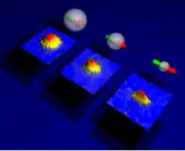
single wave packets begin to overlap until a zero temperature, where all of these occupy the same quantum ground state and it is represented for a singular macroscopic wave function. This phenomenon is called Bose-Einstein condensation (Figure 1). It is worth noting in addition to low temperatures, the formation of a condensate needs a dilute gas to reduce the three body collisions, because these create a high kinetic energy giving rise to a heating and hence losses which depend on the atomic density. Thus in a dilute gas only collisions between two particles are relevant. In other words, the dilution condition
∗Bradley et al., besides the BEC formation they also show the collapse evidence in a BEC. Curiously only
Figure 1: On the left side is shown the phase transition from an ideal gas to a BEC (http://cua.mit.edu/ketterle_group/intro/whatbec/whtisbec.html). The right side shows the velocity distribution of 87Rb with a field of view 200µm × 270µm. The images are at 400nK (just above condensation), 200nK (after the condensation) and 50nK (af-ter further evaporation leaves a sample of nearly pure condensate) respectively from left to rigth. The red color corresponds to the least amount of atoms but the fastest and so on until the white color to the largest number of atoms and the slowest (http://jila.colorado.edu/bec/CornellGroup/gallery/images/BEC_peaks.jpg).
at low energies could be interpreted such that the effective interaction between particles may be characterized by a single quantity, the scattering length a [2], thus the gases are dilute in the sense that the scattering length is much less than the interparticle spacing.
The huge interest in the ultracold gases field allowed in 2005 the experimental realization of a 52Cr Bose-Einstein condensate with inter-atomic magnetic dipole dipole interaction [10], opening the door to a new level in the degenerate quantum gases research. The rich-ness of the new interaction is accompanied by a more complicated theoretical treatment as opposed to the contact interaction, this is because of its two new features, the long-range character and the anisotropy† (being partially repulsive or attractive). Those new
properties attracted much interest, both theoretically and experimentally in the last 10 years ([11, 12, 13] and references therein), providing the possibility of controlling interpar-ticle interactions either by tuning external fields or else by adjusting the trap anisotropy [11, 12, 14, 15, 16]. An interesting phenomenon and in analogy with the collapse in a non-dipolar condensate it was observed in a dipolar BEC (DBEC) with Chromium called the d-wave Bose-nova [17] where the theoretical description using simulations of the full GPE including the three-body losses agrees with the experimental results [16, 17].
This dissertation presents a basic description about of the most relevant features of a dipolar condensate. As part of the study is included the non-dipolar condensate to com-pare these results with those produced by the dipolar one. For a dipolar condensate are described the main ideas about the long-range character and the anisotropy of the in-teraction, the non-local mean-field GPE [11, 12], the TF approximation [2, 11, 13], and an overview of the hydrodynamic viewpoint [13] (contains a broad development about the hydrodynamics in a dipolar condensate). The main subject is focused in the numer-ical and variational study of the existence of bright solitons in a quasi-one-dimensional dipolar condensate. The results achieved are compared with those produced by the three-dimensional condensate.
The dissertation is organized as follows. The first Chapter shows a review of basic elements of Hartree approximation and the mean-field theory to get the Gross-Pitaevskii equation. Likewise as method to solving the GPE is applied the conventional Gaussian variational ansatz for a spherical symmetry in both regimes attractive and repulsive. The most relevant information is given for the repulsive interaction because here it is possible to find the critical parameter below which the condensate should collapse. The Thomas-Fermi (TF) approximation is included too. This is physically justified for sufficiently large clouds in which the interaction and the trap energy are larger than the kinetic energy, thus this latest contribution can be neglect in the GPE. The next Chapter leads the hydrodynamic viewpoint of a BEC, with a general but complete deduction of the density equation and superfluid velocity along with the physical implications established for the quantum nature of the condensation reflected in the appearance of the quantum pressure as opposed with the classical treatment of a fluid. The last part of Chapter includes a simple example of elementary excitations in a uniform gas in order to observe the effect of the contact
†By exploring this feature, the Stuttgart group was able to characterize the presence of the dipole dipole
interaction because the alignment of dipoles respect to the trap axes changes the aspect ratio ωz/ωx orωz/ωy
interaction in the energy spectrum of the condensate. In particular, it is shown that the attractive interaction constrains the existence of the spectrum. The third Chapter is designed to the dipole dipole interaction emphasizing its main features, the anisotropy and the long-range character. Again by means of a mean-field theory is described a dipolar condensate with the non-local GPE or dipolar GPE (DGPE). The effect of the dipolar interaction also is analized in the TF approximation. In a same way from the hydrodynamic theory are shown the different intervals of existence in the spectrum of energy of a homogeneous dipolar condensate some of which contrasting with the non-dipolar case. The fourth Chapter introduces the soliton theory in a BEC. As first insight of the possible existence of the soliton in a condensate is used the modulational instability in the quasi-one-dimensional model. This equation is achieved using dimensional reduction from the three- to one-dimension in the full GPE. The theory of differential equations allows the existence of analytical solutions of the quasi-1D GPE without trap, called dark and bright solitons for repulsive (a > 0) and attractive (a < 0) interactions respectively. The present dissertation is focused in bright solitons. The end of Chapter is devoted to the collapse in a three-dimensional BEC with attractive interactions without trap in the z direction. It is used a variational approximation for two different ansatz, a Gaussian function and a bright soliton-like function. In this study were found analytical expressions to the variational parameters as function of the product of the number of particles and the scattering lengthN a. Those analytical results agree with the numerical calculations. The last Chapter is a compilation of the different tools developed along the dissertation applied to three dipolar condensates of experimental interest, 52Cr, 168Er and
164Dy. The study is performed to the three- and quasi-one-dimensional condensates under
Contents
Abstract iii
Abstract iv
Introduction v
1 The Gross–Pitaevskii equation 1
1.1 A dilute quantum gas . . . . 1
1.2 The GPE from the Hartree Approximation . . . . 3
1.3 The GPE in the mean-field approximation . . . . 7
1.4 Approximate solutions to the time-independent GPE . . . . 9
1.4.1 Variational solution . . . . 9
1.4.2 The Thomas–Fermi approximation . . . . 12
2 The hydrodynamic theory of a BEC 17 2.1 The hydrodynamic equations . . . . 17
2.2 Elementary excitations . . . . 20
3 Dipolar Bose-Einstein condensate 24 3.1 Magnetic and Electric dipole dipole interaction . . . . 25
3.1.1 Magnetic dipole dipole interaction. . . . . 25
3.1.2 Electric dipole dipole interaction. . . . 26
3.2 Dipolar interaction . . . . 27
3.3 Dipolar Gross-Pitaevski equation . . . . 30
3.4 Thomas-Fermi approximation for the DGPE . . . . 32
3.5 The hydrodynamic equations . . . . 35
3.5.1 Homogeneous gas: phonon instability . . . . 36
4 Solitons in a BEC 41 4.1 The soliton . . . . 41
4.2 The nonlinear Schrödinger equation . . . . 43
4.2.1 The NLSE in a BEC . . . . 43
4.3 GPE reduction from 3D to 1D . . . . 44
CONTENTS
4.5 Dark and bright solitons in the quasi-one-dimensional GPE . . . . 47
4.5.1 Static dark solitons . . . . 48
4.5.2 Moving dark solitons . . . . 49
4.5.3 Bright solitons . . . . 54
4.6 Collapse of a BEC with attractive interactions . . . . 59
4.6.1 Variational approximation and numerical results . . . . 59
5 Quasi-one-dimensional dipolar BEC 65 5.1 Reduction from 3D to 1D in the DGPE . . . . 65
5.2 Variational approximation . . . . 66
5.3 Existence of bright solitons and instability by collapse . . . . 69
5.3.1 Collapse of a 3D dipolar condensate . . . . 69
5.3.2 Variational approximation and numerical results . . . . 70
5.3.3 Collisions of bright solitons in a quasi-1D dipolar condensate . . . . 77
Summary and conclusions 81 Appendix 83 A Deduction of the GPE 83 A.1 The GPE from Schrödinger equation in the Hartree approximation . . . . 83
A.2 Derivation of the GPE in the mean-field approximation . . . . 85
B Fourier transform of the dipolar interaction 86 B.1 First method . . . . 86
B.2 Second method . . . . 87
C Virial theorem in Bose-Einstein condensation 89 C.1 Virial theorem of a BEC . . . . 89
C.2 Virial theorem of a dipolar BEC . . . . 90
D Modulational instability 91 E Useful math tools 93 E.1 Integrals . . . . 93
E.2 Cubic equation . . . . 93
F Quasi-one-dimensional dipolar interaction 96
Chapter 1
The Gross–Pitaevskii equation
This Chapter introduces the Gross-Pitaevskii equation (GPE) to describe a Bose-Einstein condensate (BEC) confined in a trap to zero temperature [2, 3, 4, 9]. The gas is considered highly diluted allowing approximate the interaction potential between particles like an effective contact term [18, 19]. Will be featured the most relevant aspects to the GPE deduction in both the Hartree and the mean-field approximation. In a same way by means of a variational approximation and using the Thomas-Fermi regime are shown the first insights about the approximate solutions of the mean-field GPE.
1.1
A dilute quantum gas
The dilute quantum gases [2] differ from ordinary gases, liquids and solids in different ways. The density of molecules in the air at room temperature and atmospheric pressure is about 1019cm−3, in liquids and solids the density of atoms is of order 1022cm−3, and at
center of the condensate the particle density is typically (1013−1015) cm−3. To observe
quantum phenomena at low density the temperature must be 10−5K or less. This
con-trasted with the temperatures at which quantum phenomena occur in solids and liquids. For electrons in metals the quantum effects become strong below the Fermi temperature, which is typically (104−105) K, and for phonons these are appreciable below the Debye temperature, which is of order 102K.
par-1.1. A DILUTE QUANTUM GAS
ticles N in a volume |a|3 [3]. This can be written as n|a|3, with n the average density of the gas. Experimentally the atomic scattering lengths used in the first BECs are:
a= 5.77nm for87Rb,a=−1.45nm for7Li anda= 2.75nm for23Na. The density range is (1013−1015) cm−3 then n|a|3
<10−3. So, since n|a|3
≪1, the system is called dilute or weakly interacting. However, this quantity doesn’t imply necessarily that the interaction effects are small, because these have to be compared with the kinetic energy of the atoms in the trap. The parameter that allows this comparison is given by N|a|/aosc such that
this can be larger than 1 even if n|a|3 ≪1 and thus the gas behavior can be non ideal.
The two body effective interaction
In an identical bosons gas at very low temperature and dilute the only open scattering channel is the s-wave channel, this means that the relevant two body collisions have rel-ative angular momentum between atoms equal to zero [20].
The experimental relevance achieved by the alkali atoms in the condensation is based in the interaction potential. The exact description of the interaction potential has a repulsive hard core, it is very deep with a minimum at a distance r and it contains many bound states corresponding to molecular states for two alkali atoms which aren’t typically confined by the trap due to the total spin 0. Thus, the leading disadvantages to use the exact interaction potential are [18]:
• The potential is very difficult to calculate and a small error in this may result in a large error on the scattering length.
• The potential cannot be treated in the Born aproximation because it is very strongly repulsive at short distances and it has many bound states (for a potential as soft as a square well of radius r, the Born approach applies when the zero point energy for confinement ~2/2M r2 (M the reduced mass), is much larger than the potential depth, which implies the nonexistence of bound state in the well).
1.2. THE GPE FROM THE HARTREE APPROXIMATION
aBorn =
M
2π~2
ˆ
drV (r) (1.1)
From this expression, the low energy scattering behavior may be obtained by using of an effective interaction Vef f. So
2π~2
M aBorn = ˆ
drVef f (r)≡g (1.2)
for particles with the same mass m, this result becomes
g = 4π~
2a
m (1.3)
Thus the effective interaction between two particles at low energies in coordinate space corresponds to a pseudopotential [22] or contact interactionVcontact(r) = gδ(r−r′), where
r and r′ are the positions of the two particles.
Oscillator scale length aosc
One relevant feature of the trapped Bose gases is its inhomogeneity and its finite size, where the number of atoms varies from a few thousands to several millions. As in most cases the confining traps are approximated by harmonic potentials, the trapping frequency
ω0 provides a natural scale of the system, and the oscillator length a0 = (~/mω0)1/2 is a natural length scale. This is of the order of a few microns in the available samples and can be used to simplify the problem. The unidimensional time-independent Schrödinger equation for the harmonic oscillator in terms of the new variable x−→x/a0 can be writ-ten as the dimensionless Schrödinger equation
1 2
" − d
2
dx2 +x 2
#
ψ(x) = E
~ωψ(x) (1.4)
In general for three dimensions the oscillator scale length is given by
aosc =
~
mωosc
!1/2
(1.5)
Defining the geometric average of the oscillator frequencies as ωosc= (ωxωyωz)1/3 [3].
1.2
The GPE from the Hartree Approximation
1.2. THE GPE FROM THE HARTREE APPROXIMATION
φ(r, t) and thereby the wave function of the N particles system Ψ (r1,r2, ...,rN, t) may
be written like [2, 4]
Ψ (r1,r2, ...,rN, t) =
N
Y
i=1
φ(ri, t) (1.6)
with the single-particle wave function normalization such that
ˆ
dr|φ(r, t)|2 = 1 (1.7)
The other hand, the effective Hamiltonian of a N particles system with the same mass is
H =
N
X
i=1
"
p2i
2m +V (ri)
#
+g
N
X
i<j
δ(ri−rj) (1.8)
Where pi is the momentum of a particle in the positionri. V (ri) is an external potential. The last term corresponds to the contact interaction between two particles. One of the ways to get the motion equation implies the product of the Schrödinger equation byN−1 single-particle wave functions and the integration over these N −1 functions. Thus,
i~∂
∂t
N
Y
i=1
φ(ri, t) =H N
Y
i=1
φ(ri, t) (1.9)
i~
NY−1
j=1 ˆ
drjφ∗(rj, t) ∂
∂t
N
Y
i=1
φ(ri, t) =
NY−1
j=1 ˆ
drjφ∗(rj, t)H
N
Y
i=1
φ(ri, t) (1.10) The result is the non-linear Schrödinger equation for a single-particle wave function (for more details see the Appendix A.1)
i~∂
∂tφ(rj, t) =−
~2 2m∇
2φ(r
j, t) +V (rj)φ(rj, t) +g(N −1)|φ(rj, t)|2φ(rj, t) (1.11)
Now, defining the condensate wave function like Ψ (r, t) = N1/2φ(r, t), the density of
particles is given by
n(r) =|Ψ (r, t)|2 (1.12)
and the condition for the total number of particles turns into
N =
ˆ
dr |Ψ (r, t)|2 (1.13)
So with the wave function Ψ (r, t) and the approximationN ≫1, the non-linear Schrödinger equation for the condensate (1.11) becomes [2, 3, 4]
i~∂Ψ (r, t)
∂t =−
~2 2m∇
2Ψ (r, t) +V (r) Ψ (r, t) +g
1.2. THE GPE FROM THE HARTREE APPROXIMATION
describes the zero-temperature properties of a non-uniform Bose gas whereas the num-ber of atoms in the condensate N is much larger than 1 and the scattering length a is much less than the average distance between atoms or also called weak-coupling limit
n|a|3 ≪1. In the strong-coupling regime n|a|3 ≫1 the GPE highly overestimates the atomic contact interaction and leads to unphysical results (references therein [23]). An important feature in the GPE is given by the sign of scattering lengtha, whilea >0 it corresponds to an effective repulsion and if a <0 it corresponds to an effective attraction. This dissertation gives more attention to the attractive case.
From theoretical viewpoint is easier dealing with a dimensionless model. So, taking the GPE with dimensions in terms of variables Φ (˜r, τ), ˜r and τ
i~∂Φ (˜r, τ)
∂τ =−
~2 2m∇
2Φ (˜r, τ) +V (˜r) Φ (˜r, τ) +gN|Φ (˜r, τ)|2
Φ (˜r, τ) (1.15) where the normalization and the density of particles number respectively are
ˆ
d˜r |Φ (˜r, τ)|2 = 1 (1.16)
n(˜r) =N|Φ (˜r, τ)|2 (1.17)
Likewise in theoretical works is conventional to use a harmonic potential as
V (˜r) = 1 2m
˜
ω2xx˜2+ ˜ωy2y˜2+ ˜ω2zz˜2 (1.18) To obtain a dimensionless GPE [24] is defined the variables change r = ˜r/aosc, or
x = ˜x/aosc, y = ˜y/aosc, z = ˜z/aosc. In a same way ωx2 = ˜ωx2/ωosc2 , ωy2 = ˜ωy2/ωosc2 ,
ωz2 = ˜ω2z/ωosc2 , with aosc= (~/mωosc)1/2. Also t=τ ωosc, and Ψ (r, t) = a3osc/2Φ (˜r, τ), thus
∂Φ (˜r, τ)
∂τ =
ωosc
a3osc/2
∂Ψ (r, t)
∂t and ∇
2Φ (˜r, τ) = 1 a3osc/2
"
1
a2
osc∇
2Ψ (r, t)
#
(1.19)
Hence the GPE (1.15) takes the form
i~ωosc
a3osc/2
∂Ψ (r, t)
∂t =
" − ~
2
2ma2
osc
∇2+ 1 2ma
2
oscωosc2
ωx2x2+ωy2y2+ωz2z2
+ 4π~
2N˜a ma3
osc |
Ψ (r, t)|2
#
Ψ (r, t)
a3osc/2
(1.20)
Or simple way
i∂Ψ (r, t)
∂t =
−1
2∇
2+V (r) + 4πaN|Ψ (r, t)|2
Ψ (r, t) (1.21)
1.2. THE GPE FROM THE HARTREE APPROXIMATION
V (r) = 1 2
ωx2x2+ωy2y2+ωz2z2 (1.22) Is common to express the potential in a cylindrical symmetry as follows
V (r) = 1 2ω
2 ⊥
ρ2+λ2z2 (1.23)
with ω⊥2 = ωx2 =ω2y, ρ2 =x2+y2 and λ= ωz/ω⊥. This parameter defines three types of
condensates. For λ = 1 the condensate is spherical. For λ > 1 it is referred as disk- or pancake-shaped where the width in z smaller than width along ρ. For λ <1 the conden-sate is cigar-shaped and it is more larger in the z direction than in the radial. In a same way the normalization of the wave function and the condensed density respectively are
ˆ
dr|Ψ (r, t)|2 = 1 (1.24)
n(r) = N|Ψ (r, t)|2 (1.25)
In a first insight the GPE (1.21) looks like an eigenvalue equation, where the eigenvalue could be the energy given by the expectation value for H′
i∂Ψ (r, t) ∂t =
−12∇2+V (r) + 4πaN|Ψ (r, t)|2
| {z }
H′
Ψ (r, t) (1.26)
However it is not completely correct because of the presence of the interaction energy which it is counted twice. The energy asocciated to the interaction term is the chemical potential according to the thermodynamic relation µ= ∆E/∆N. Thus,
i∂Ψ (r, t) ∂t =H
′Ψ (r, t) =µΨ (r, t) (1.27)
with the solution
Ψ (r, t) = Ψ (r) exp (−iµt) (1.28)
Then the chemical potential is the eigenvalue to the GPE do not the energy per particle like this it is for the Schrödinger linear equation. Using the solution Ψ (r, t) in the GPE (1.21) the time-independent behavior of the condensate is given by
µΨ (r) =
−1
2∇
2 +V (r) + 4πaN|Ψ (r)|2
Ψ (r) (1.29)
From the wave function normalization ´
dr|Ψ (r)|2 = 1 the chemical potential of a BEC
can be calculated as
µ=
ˆ
drΨ∗(r)
−1
2∇
2+V (r) + 4πaN|Ψ (r)|2
Ψ (r) (1.30)
1.3. THE GPE IN THE MEAN-FIELD APPROXIMATION
H =H′−2πaN|Ψ (r, t)|2 =−1
2∇
2+V (r) + 2πaN|Ψ (r, t)|2
(1.31)
and using the condensed wave function (1.28) the accurate hamiltonian to obtain the energy is
H = −1 2∇
2+V (r) + 2πaN
|Ψ (r)|2 (1.32)
The Hamiltonian expectation value corresponds to the energy of a particle and the total energy of the condensate can be written as
E(Ψ) =
ˆ dr
1
2N|∇Ψ (r)|
2
+V (r)N|Ψ (r)|2+ 2πaN2|Ψ (r)|4
(1.33)
with the respective energies on the condensate
Ekin =
1 2
ˆ
drN|∇Ψ (r)|2 (1.34)
Eint = 2π
ˆ
draN2|Ψ(r)|4 (1.35)
Etrap=
ˆ
drV (r)N|Ψ(r)|2 (1.36)
The chemical potential (1.30) may also be obtained from the energy (1.33) using the ther-modynamic relation µ=∂E/∂N. Or alternatively as
µ= 1
N (Ekin+Etrap+ 2Eint) (1.37)
Thus for non-interacting particles all in the same state the chemical potential has the same value that the energy per particle. A further important relationship can be found by means of the virial theorem (Appendix C.1). This allows to testing the accuracy of a numerical algorithm. So
2Ekin+ 3Eint−2Etrap = 0 (1.38)
1.3
The GPE in the mean-field approximation
Another way to get the GPE implies the use of second quantization and the Bogoliubov approach for a system of many interacting bosons, i.e. taking the Heisenberg equation with the boson fields operators and the Bogoliubov consideration [3]. The many-body Hamiltonian in second quantization describing N interacting bosons confined by an ex-ternal potential is given by
ˆ
H =
ˆ
drΨˆ†(r, t) ˆH0Ψ (ˆ r, t) + 1 2
ˆ
1.3. THE GPE IN THE MEAN-FIELD APPROXIMATION
With the single particle operator
ˆ
H0 =−~
2
2m∇
2+V (r) (1.40)
the two-body interatomic potential V (r−r′) and the creation and annihilation boson fields operators ˆΨ†(r) and ˆΨ (r) respectively. These obey the usual commutation relations
h
ˆ
Ψ (r, t),Ψˆ†(r′, t)i=δ(r−r′) (1.41)
h
ˆ
Ψ (r, t),Ψ (ˆ r′, t)i= 0 (1.42)
h
ˆ
Ψ†(r, t),Ψˆ†(r′, t)i= 0 (1.43) To the effective interaction between two particles the hamiltonian takes the form
ˆ
H =
ˆ
drΨˆ†(r, t) ˆH0Ψ (ˆ r, t) + g 2
ˆ
drdr′Ψˆ†(r, t) ˆΨ†(r′, t)δ(r−r′) ˆΨ (r′, t) ˆΨ (r, t)
=
ˆ
drΨˆ†(r, t) ˆH0Ψ (ˆ r, t) + g 2
ˆ
drΨˆ†(r, t) ˆΨ†(r, t) ˆΨ (r, t) ˆΨ (r, t) (1.44)
in the Heisenberg picture the dynamics of the system is given by
i~∂
∂tΨ (ˆ r
′, t) = hΨ (ˆ r′, t),Hˆi (1.45)
Therefore, the result is a field operators equation (for more details see (A.2))
i~∂
∂tΨ (ˆ r ′, t) =
" − ~
2
2m∇
2+V (r′) +gΨˆ†(r′, t) ˆΨ (r′, t)
#
ˆ
Ψ (r′, t) (1.46) Finally, using the Bogoliubov approach [2, 4] according to which since the condensate state involves the macroscopic occupation of a single state it is appropriate to decom-pose the Bose field operator in terms of a macroscopically populated mean field term
D
ˆ
Ψ (r′, t)E = Ψ (r′, t) and taking into account small fluctuations (quantum or thermal)
about the condensate state δΨ (ˆ r′, t). Thus, ˆ
Ψ (r′, t) = Ψ (r′, t) +δΨ (ˆ r′, t) (1.47) Taking only the leading order terms in Ψ (r′, t)∗ the time-dependent GPE is given by
i~∂
∂tΨ (r, t) =
" −~
2
2m∇
2+V (r) +g|Ψ (r, t)|2
#
Ψ (r, t) (1.48)
∗It would be wrong to replace ˆΨ (
r, t) with Ψ (r) for a realistic potential [4]. However, the change is accurate if
(i) the effective potentialV (r) is soft where the Born approximation is applicable. It is true when the scattering
length is less than the thermal de Broglie wavelengtha≪λB ≈ ~/(mkBT)
1/2
withmthe mass of the particle andkBthe Boltzmann’s constant.(ii) The temperature is much less than the transition temperature for the onset
1.4. APPROXIMATE SOLUTIONS TO THE TIME-INDEPENDENT GPE
For the stationary states in the GPE the wave function evolves in time in a same way like the ansatz Ψ (r, t) = Ψ (r) exp (−iµt/~). The phase factor reflects the fact that microscopically Ψ (r, t) is equal to the matrix elements of the annihilation operator ˆΨ (r, t) in Heisenberg picture between the ground state with N particles and that with N −1
particles [2] D
ˆ
ΨE= Ψ (r, t) =DN −1Ψ (ˆ r)N E
(1.49)
Ψ (r, t) = DN −1eiHt/ˆ ~ˆ
Ψ (r)e−iHt/ˆ ~
NE∝e−i(EN−EN−1)t/~
(1.50)
For a large particle numbers N, it is possible to perform the approximationEN−EN−1 ∼ ∂E/∂N which is equal to the chemical potential µ. So, in a same way like it was done above with the dimensionless GPE (1.21), the chemical potencial and the total energy of the condensate correspond with (1.30) and (1.33) respectively.
1.4
Approximate solutions to the time-independent GPE
Now will be examined some solutions of the GPE for bosons in a trap [2, 3, 4]. Due to the experimental relevance will be considered harmonic traps V (r), but the formalism may be applied to more general traps.
1.4.1 Variational solution
The variational method is one way of find approximations to the lowest energy eigenstate or ground state. The idea consists in take a trial function with a fixed shape but some free parameters and finding the values of these parameters for which the expectation value of the energy is the lowest possible. The expectation value of the energy in the new state is an upper bound to the ground state energy. If the shape of the actual solution is close to the trial function, the results obtained with the variational method will be in good agreement with the real solutions, but in other cases the method can be very rough or even fail.
In the weak coupling limit (N a→0) the interaction contribution is small and it may be neglected, thus the system matches with a harmonic oscillator like (1.4). In three di-mensions, the lowest single-particle state to the harmonic oscillator has a Gaussian form as
φ0(r) = 1
π3/4 e−
r2
/2 (1.51)
wherer2 =x2+y2+z2. Now, will be taken as normalized trial function the same gaussian form for the condensate wave function Ψ (r), such that
Ψ (r) =
1
w3π3/2
1/2
1.4. APPROXIMATE SOLUTIONS TO THE TIME-INDEPENDENT GPE
As the presence of the interatomic interactions change the dimensions of the cloud then is useful to take as dimensionless variational parameter the length w which fixes the width of the condensate [25]. A variational solution with a more general wave function to the time-dependent GPE is presented by Salasnich [26].
The substitution from normalized trial function (1.52) into the condensate energy (1.33) yields the contributions†
|Ψ(r)|2 = 1
w3π3/2 e−
r2
/w2
(1.53)
|Ψ(r)|4 = 1
w6π3 e− 2r2
/w2
(1.54)
|∇Ψ(r)|2 = 1
w3π3/2
r
w2
2
e−r2/w2 (1.55)
For a spherical trap V (r) (λ = 1 in (1.23) and for easily taking ω⊥= 1), the potential is given by
V (r) = 1 2r
2 (1.56)
Thus the total energy of the condensate takes the form
E = N
ˆ dr " 1 2 1
w3π3/2 e−
r2
/w2 r
w2
2
+ 1 2r
2 1 w3π3/2 e−
r2
/w2
+ 2πaN 1 w6π3e−
2r2
/w2
#
= N
2w3π3/2
1
w4 + 1
ˆ
drr2e−r2/w2 +2πaN
2
w6π3
π
2
3/2 w3
= 3
4
N w3π3/2
πw61/2πw2 1 w4 + 1
+ 2πaN
2
w3
1
2π
3/2
= 3
4N
1
w2 +w
2+ aN2
(2π)1/2w3 (1.57)
The chemical potential can be obtained from µ=∂E/∂N
µ(w) = 3 4
w2+ 1
w2
+
2
π
1/2 N a
w3 (1.58)
and the total energy per particle turns into [2, 3, 4]
E(w)
N =
3 4
w2+ 1
w2
+ √1
2π N a
w3 (1.59)
N a is a measure of the strength of the atom-atom interaction expressing its importance
†Useful integrals
´∞
−∞e −bx2
dx=pπ
b b >0
´∞
−∞x
2
e−bx2
dx=1 2
pπ
1.4. APPROXIMATE SOLUTIONS TO THE TIME-INDEPENDENT GPE
compared to the kinetic energy. In most experiments on atoms with repulsive interactions,
N a is much larger than unity [3]. In the first experiments with rubidium atoms at JILA (1995) the ratio|a| ∼7×10⁻³withN a few thousands, thenN|a|>1. In the experiments
with 7Li at Rice University (1995) the number of particles is of the order of 1000 and
|a| ∼ 0.5× 10⁻³ and N|a| > 1. In the experiments with sodium at MIT (1995) the
number of atoms in the condensate is very large 106−107 and N|a| ∼103 −104.
The Figure (1.1) illustrates the energy per particle E/N (1.59) in the variational treat-ment of a condensate like function of the variational parameter w for different values of the parameter N a. The curveN a = 0 shows the behavior of the ground state of the sys-tem without interactions which is equivalent with a three-dimensional isotropic harmonic oscillator and the corresponding energy per particle is equal to 3/2. For repulsive intera-cions (a >0) the energy per particle always has a minimum indicating the existence of a stable ground state. The other hand, a local minimum exists for attractive interactions when N is less than some critical value of particle number Nc [2, 3, 4, 27], but for larger
values of N the cloud will collapse, this is the case of the 7Li [6]. The Nc satisfies that
both the first and second derivative of E/N with respect to the variational parameter w
are equal to zero. So using the energy per particle (1.59) for attactive interactions (a <0)
E N =
3 4
1
w2 +w
2−√1
2π N|a|
w3 (1.60)
-2
0
2
4
6
8
0.0 0.5 1.0 1.5 2.0 2.5
w
−
0
.
3
−
0
.
67
−
1
0
N a
= 1
E/N
1.4. APPROXIMATE SOLUTIONS TO THE TIME-INDEPENDENT GPE
Deriving E/N respect to the variational parameter w and equaling to zero 3
4
2w− 2
w3
+√3
2π N|a|
w4 = 0 (1.61)
s
2
πN|a|=w−w
5 (1.62)
To the second one derivate and again equaling to zero
3 4
2 + 6
w4
− √12
2π N|a|
w5 = 0 (1.63)
w5+ 3w= 4
s
2
πN|a| (1.64)
When the equations to the first and the second derivate (1.62) and (1.64) are equal to each other, the critical variational parameter is
wc =
1
5
1/4
(1.65)
Using this critical parameter in (1.64) the critical value of particle number is given by
Nc|a|=
1 4
rπ
2
"1
5
5/4
+ 3
1
5
1/4#
(1.66)
Thus, [2, 3, 25]
Nc|a|=
(8π)1/2
55/4 ≈0.671 (1.67)
A numerical integration of the GPE gives Nc|a| = 0.575 [28, 29]. The other hand,
when the spherical trap frequency is different to 1, the critical parameter is given by
Nc|a|≈0.671/ω⊥1/2.
1.4.2 The Thomas–Fermi approximation
1.4. APPROXIMATE SOLUTIONS TO THE TIME-INDEPENDENT GPE
n(r) =N|Ψ (r)|2 = µ−V (r)
4πa (1.68)
This equation is valid when n(r) > 0 and it gives the size of the cloud if µ = V (r). Therefore the energy to add a particle at any point in the cloud is the same everywhere and the density profile is completely determined by the trapping potential.
In the TF approximation for a spherical trap, the energy can be calculated as follows. In this approximation the radius of the condensate is defined by R and it is obtained using the harmonic potential (1.56) and the condition µ=V (r), so
R2 = 2µ (1.69)
According to the normalization condition of the wave function (1.24) the chemical poten-tial is fixed and it is relationed with the total number of particles
N =
ˆ
drN|Ψ (r)|2
= µ
4πa ˆ
dr 1− V
µ
!
= µ
4πa ˆ
dr
"
1− r
2
R2
#
Integrating inside a sphere of radius R
1 = µ
4πaN
4
3πR
3− 4
5πR
3= 2
15
µ aNR
3 (1.70)
and using (1.69)
1 = 2 15
µ aN (2µ)
3/2
(1.71)
the chemical potential is
µ= 15
2/5
2 (N a)
2/5
(1.72)
The Figure (1.2) compares the trial wave function in the variational study (1.52) for a variational parameter equal to 1, with the TF solution (1.68) for a spherical trap (1.56) and using the chemical potential given by (1.72). In the TF regime the condensate has well defined edges and from the chemical potential (1.72), the radius of the condensate (1.69) can be given in terms of the strength of the atom-atom interaction N a as
1.4. APPROXIMATE SOLUTIONS TO THE TIME-INDEPENDENT GPE
0.0
0.1
0.2
0.3
0.4
0.5
0.0 0.5 1.0 1.5 2.0 2.5 3.0
r/α
Ψ
Gaussian
T homas
−
F ermi
Figure 1.2: The full line is the ground state wave function for the Gaussian variational solution and the dotted line is the TF approximation to an isotropic harmonic oscillator potential. The wave functions are in unitsα= (N a)1/5, thus the variable change is Ψα3/2→Ψ.
The energy of the condensate in the TF approximation can be calculated according to the usual thermodynamic relation µ=∂E/∂N from (1.72)
E = (15a)
2/5
2
ˆ N 0
dN′N′2/5 = 5 7
(15a)2/5
2 N
7/5 (1.74)
The energy per particle can be written like
E N =
5 7
(15)2/5 2 (N a)
2/5
(1.75)
So in terms of the chemical potential (1.72) the energy per particle in the TF regime has the form [2]
E N =
5
7µ (1.76)
1.4. APPROXIMATE SOLUTIONS TO THE TIME-INDEPENDENT GPE
respect to the variational parameter. The minimization is given in the same way as the equation (1.62), thus
w5 =
s
2
πN a (1.77)
Then, the energy per particle for the TF approximation turns into
E
N =
3 4
2
π
1/5
(N a)2/5+1 2
2
π
1/5
(N a)2/5 (1.78)
E
N =
5 4
2
π
1/5
(N a)2/5 (1.79)
In the Figure (1.3) the minimum energy per particle in the TF regime obtained from the variational approximation (1.79) within the range of stability N a ≥ −0,67 is compared with the TF approximation (1.75). From these results, the TF energy per particle in the variational treatment is greater than the TF energy (1.75) as expected. The rate is given by a factor 7/(3600π)1/5 ≈1,08.
0
1
2
3
0
2
4
6
8
10
N a
E/N
Gaussian
T homas
−
F ermi
1.4. APPROXIMATE SOLUTIONS TO THE TIME-INDEPENDENT GPE
The TF approximation lets see how the total energy is distributed between potential and interaction energies. For this is necesary insert the TF solution (1.68) with a spherical potential (1.56) into the energies in (1.35) and (1.36), neglecting the kinetic contribution (1.34). So
Eint= 2πa
ˆ
drN2|Ψ (r)|4 = 1 8πa
ˆ
dr µ2−2µV +V2 (1.80) Using the volume integral in a spherical coordinates with radius R. To the first term
µ2 ˆ
dr = 4π 3 µ
2R3 (1.81)
To the second one
2µ ˆ
drV = 4πµ ˆ
dr r4 = 8π 5 µ
2R3 (1.82)
To the third one
ˆ
drV2 =π ˆ
dr r6 = π 7R
7 = 4
7πµ
2R3 (1.83)
Adding those three contributions the resulting interaction energy per particle is
Eint =
4 105
µ2R3 a
!
(1.84)
In a same way the trap energy or the oscillator energy per particle is
Etrap =
ˆ
drV (r)N|Ψ (r)|2 =
ˆ
drV (r)
"
µ−V (r) 4πa
#
= 2
35
µ2R3 a
!
(1.85)
The ratio between these energies is given by
Eint
Etrap
= 2
3 (1.86)
Since the total energy in the TF approximation is E = 5µ/7 (1.76) and
E =Eint+Etrap (1.87)
Furthermore, using the ratio between interaction and trap energy (1.86) the energy dis-tribution in the TF approximation is
Eint =
2
7µ Etrap=
3
Chapter 2
The hydrodynamic theory of a BEC
The collective modes and the expansion of the condensed cloud when released from a trap are important sources of physical information for a better description of the BEC. The behavior of these phenomena is investigated by means of the time-dependent GPE [2, 4]. Using this mean-field equation (1.21) may be derived useful equations very similar to those of classical hydrodynamics that represent the conservation laws for the number of particles and the total momentum (an extensive description about the hydrodynamic in a condensate may be found in [13]).
2.1
The hydrodynamic equations
The hydrodynamic as macroscopic theory can be used to studying the superfluid behavior at zero temperature of a BEC. The link between a superfluid and a condensate is given by means of the definition of the superfluid velocity [19]. Nevertheless, in the hydrodynamic description it is not appropriate to deal with the time-dependent GPE to research the superfluid macroscopic state, instead it is better to use equivalent equations for the density and the gradient phase [9].
The mean-field GPE has like a conserved quantity the total number of particles such that
dN/dt = 0, therefore it is possible considering a continuity equation reflecting this fact. Thus performing the product of the time-dependent GPE (1.21) by NΨ∗(r, t) and
sub-tracting the complex conjugate of the new equation it is obtained the continuity equation
∂ ∂t
N|Ψ|2− i
2∇ ·[N(Ψ
∗∇Ψ−Ψ∇Ψ∗)] = 0 (2.1)
with the particles density n =N|Ψ|2. Defining the local velocity as
v = −i 2
(Ψ∗∇Ψ−Ψ∇Ψ∗)
|Ψ|2 (2.2)
2.1. THE HYDRODYNAMIC EQUATIONS
∂n
∂t +∇ ·j = 0 (2.3)
The density may be obtained using the ansatz Ψ (r, t) = [n(r, t)/N]1/2exp [iφ(r, t)] (the phase φ(r, t) is a real quantity) on the GPE (1.21) such that
i
"
∂√n ∂t e
iφ+i√n∂φ
∂te
iφ
#
= −1
2
n
∇h∇√neiφ+i√n(∇φ)eiφio+ (V + 4πan)√neiφ
= −1
2
n
∇2√neiφ+i∇φ∇√neiφ+ih∇φ∇√neiφ
+ √n∇2φ+i(∇φ)2eiφio+ (V + 4πan)√neiφ (2.4) As the GPE is a complex equation it can be separated in a real and an imaginary part. The real contribution is given by
− ∂φ
∂t = −
1 2√n∇
2√n+ 1
2(∇φ)
2
+V + 4πan (2.5)
Introducing the ansatz Ψ (r, t) = (n(r, t)/N)1/2exp [iφ(r, t)] in the momentum density
j=nvthe condensed velocity can be defined like
v(r, t) = ∇φ(r, t) (2.6)
This velocity characterizes the behavior of a macroscopic number of particles (the con-densate) and it can thus be regarded as a classical quantity. So the real contribution becomes [2]
−∂φ
∂t = −
1 2√n∇
2√n+1
2v
2+V + 4πan (2.7)
According to the velocity (2.6), the motion of the condensate can be interpreted like a potential flow∗. If the condensed phase φ(r, t) is not singular (this condition is not
ful-filled for the core of a vortex line) the motion of the condensate is irrotational
∇ ×v=∇ × ∇φ= 0 (2.8) Now, the imaginary part in the GPE turns into
∂√n
∂t = −
1 2
2∇√n∇φ+√n∇2φ (2.9)
Multiplicand both side by √n, then 1 2
∂n
∂t = −
1 2
h
∇n∇φ+n∇2φi (2.10)
2.1. THE HYDRODYNAMIC EQUATIONS
and with the property ∇n∇φ=∇(n∇φ)−n∇2φ the imaginary part in the GPE is [2]
∂n
∂t = −∇(n∇φ) (2.11)
The motion equation for the velocity is obtained taking the gradient to the real part (2.7) and using the velocity definition (2.6). So
∂v
∂t = −∇
"
1 2v
2+V + 4πan
− 2√1
n∇ 2√n
#
(2.12)
It is more useful converting the hydrodynamics equations of the condensate as follows, with the purpose of contrasting these with the classical hydrodynamic equations. So from the thermodynamic Gibbs–Duhem relation dp = ndµ in an uniform Bose gas with chemical potential µ = 4πan the pressure is p = 2πan2. Thus, 4πa∇n = ∇p/n and the equation (2.12) takes the form
∂v
∂t = −
1
n∇p− ∇ v2
2
!
+∇ 1
2√n∇ 2√n
!
− ∇V (2.13)
The continuity equation (2.3) has the same form that for an ideal fluid, while the equation (2.13) is analogue to Euler equation
∂v
∂t + (v· ∇)v+
1
n∇p = −∇V (2.14)
Or using the vector identity
∇(A·B) = (A· ∇)B+ (B· ∇)A+A×(∇ ×B) +B×(∇ ×A) (2.15)
when A=B=v
v×(∇ ×v) = ∇ v
2
2
!
−(v· ∇)v (2.16)
So the Euler equation takes the form
∂v
∂t −v×(∇ ×v) = −
1
n∇p− ∇ v2
2
!
− ∇V (2.17)
2.2. ELEMENTARY EXCITATIONS
different. The quantum pressure (∇√n)2/2 is refered to ‘zero-point motion’, which it is not produced because of the particle currents, and ∇(v2/2) is referred to the kinetic energy of the particles motion. Definining the spatial scale of variations for the wave function like l, in the motion equation (2.13) the quantum pressure is of order 1/l3, and the pressure term is of order 4πan/l. So the usual pressure dominates on larger scales and the dynamics of the condensate can be described by the classical hydrodynamic equation. The quantum pressure dominates when the spatial variations of the density occur on length scales l less than order of the coherence length† ξ = (8πan)−1/2. As it
was described above, at zero temperature the motion of the condensate may be specified in terms of a local density and a local velocity. The equations of motion are very similar to those of a ideal fluid expressing thus the conservation of the particle number and the total momentum.
2.2
Elementary excitations
The properties of elementary excitations may be investigated using the hydrodynamic formulation [2, 4]. Writing the density as n −→ n0 +δn, where n0 is the equilibrium
density and δnis the deviation value of this equilibrium. Similarly the velocity potential becomes φ−→φ0+δφ. Dealing the velocity and the variationδnas small quantities and linearizing the density in the continuity equation (2.3) and in the Euler equation (2.12), it is possible to get that the continuity equation becomes (2.3)
∂n0 ∂t +
∂δn
∂t = −∇ ·[(n0+δn)∇(φ0+δφ)] (2.18)
Here ∂n0/∂t =−∇ ·(n0∇φ0) and the term −∇ ·[δn∇(φ0+δφ)] does not contribute in the linearization. So the new continuity equation is
∂δn
∂t = −∇ ·(n0∇δφ) (2.19)
and for the Euler equation (2.12) the phase φ0 is time constant and the velocity squared
does not contribute, so
∂
∂t(∇δφ) = −∇δµ˜ (2.20)
where δµ˜ is achieved by the linearization of ˜µ [9] with
˜
µ = V + 4πan− 1
2√n∇
2√n (2.21)
†If a uniform Bose gas is pertudrbed locally,ξ is the length over which the gas heals back to its equilibrium
density, and it can be written as 1/ 2ξ2
= 4πan. In the dilute limit na3
≪ 1, the healing length ξ is large compared to the interparticle spacingn−1/3
2.2. ELEMENTARY EXCITATIONS
The motion equation is obtained taking the time derivate in (2.19) and using the Euler equation (2.20). Thus, the equation describing the excitations of a Bose gas in an arbitrary potential is
∂2δn
∂t2 = ∇ ·(n0∇δµ˜) (2.22)
A uniform gas
In this section, it will be investigated the spectrum energy of a homogeneous BEC where the external potential is constant. The solutions sought are travelling wave such that
δn → δn exp(iq.r−iωt) where q is the wave vector and ω the frequency. Henceforth neglecting the zero-temperature depletion and to keeping the notation simple will be denoting the density of the equilibrium by n [2]. For the motion equation the term δµ˜ can be written like
δµ˜ = 4πaδn−1
2
"
δ √1
n
!
∇2√n+ √1
nδ
∇2√n
#
= 4πaδn−1
2
" −∇
2√n
2n3/2 δn+
1
√
n∇
2 δn
2√n
!#
(2.23)
Where √n is constant because in the unperturbed state the density is the same every-where. From the solution to δn then ∇2(δn) = (iq)2δn, thus
δµ˜= 4πaδn− 1
2
1
2n∇
2(δn)= 4πaδn
−12 "
(iq)2 2n δn
#
(2.24)
δµ˜= 4πa+ q
2
4n
!
δn (2.25)
and the equation of motion (2.22) takes the form
∂2δn
∂t2 =n∇
2(δµ˜) (2.26)
or
ω2 = 4πanq2 +q
4
4
!
(2.27)
With possible solutions only if ω = ±ǫq. Taking just the positive values and defining
ǫ0q =q2/2 as the free particle energy, the energy spectrum is [2, 9]
ǫq =
r
8πanǫ0
q+
ǫ0
q
2
(2.28)
2.2. ELEMENTARY EXCITATIONS
0
3
6
9
12
15
0
2
4
6
8
q/s
q
≫
0
any
q
q
≈
0
ǫ
q
/s
2
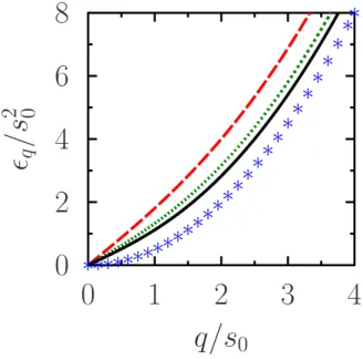
Figure 2.1: Dispersion of elementary excitations for repulsive interactions. The black line (solid curve) corresponds to the excitation spectrum of a homogeneous Bose gas as function of the dimensionless wave numberq/s. The red line (dashed curve) shows the espectrum for long wave number. The green line (dotted curve) is the approach to short wave number.
ǫq ≈ sq (2.29)
with the sound velocity s = √4πan ‡, which matches with the Bogoliubov results [30].
According to the above results the energy spectrum at long wavelengths is quadratic in q
for free particles and lineal when the repulsive interaction is present, agreement with ex-perimental observations in liquid4He. The transition between the linear and the quadratic spectrum occurs when the two pressures are very close, in other words, the kinetic energy is approximately equal to the interaction term, so q2/2∼4πan, or q = (8πan)1/2 =√2ξ−1.
For length scales longer thanξatoms move collectively and for shorter length scales these behave as free particles [2].
In the short wavelengths approximation the contribution at the energy spectrum is given by the free-particle spectrum plus a mean field shift.
ǫq =ǫ0q 1 +
8πan ǫ0
q
!1/2
≈ǫ0q
"
1 + 1 2
8πan ǫ0
q
!
+...
#
=ǫ0q+ 4πan (2.30) Or in terms of the sound velocity is
‡The speed of sound becomes purely imaginary for attractive interaction and it implies instability. A