Faraday waves in quasi-one-dimensional superfluid Fermi-Bose mixtures
F. Kh. Abdullaev,1,2M. ¨Ogren,3and M. P. Sørensen3
1Physical-Technical Institute, Uzbek Academy of Sciences, 2-b G. Mavlyanov Street, 100084 Tashkent, Uzbekistan 2Instituto de Fisica Teorica, Universidade Estadual Paulista J´ulio de Mesquita Filho, R. Dr. Bento Teobaldo Ferraz 271,
Barra Funda, S˜ao Paulo, CEP 01140-070, Brazil
3Department of Applied Mathematics and Computer Science, Technical University of Denmark, 2800 Kongens Lyngby, Denmark
(Received 27 November 2012; published 15 February 2013)
The generation of Faraday waves in superfluid Fermi-Bose mixtures in elongated traps is investigated. The generation of waves is achieved by periodically changing a parameter of the system in time. Two types of modulations of parameters are considered: a variation of the fermion-boson scattering length and the boson-boson scattering length. We predict the properties of the generated Faraday patterns and study the parameter regions where they can be excited.
DOI:10.1103/PhysRevA.87.023616 PACS number(s): 03.75.Ss, 03.75.Kk, 05.45.−a
I. INTRODUCTION
Faraday waves (FWs) are spatially periodic patterns that can be generated in a system with a periodic variation in time of the system parameters. Faraday waves were initially observed by Faraday for a vessel with a liquid oscillating in the vertical direction [1]. Such a type of structure can exist in nonlinear optical systems [2–6] where variations along the longitudinal direction of the Kerr nonlinearity can be achieved by the periodic variation of the effective cross-sectional area of the nonlinear optical fiber. Recently parametric resonances in modulational instability of electromagnetic waves in photonic crystal fibers with a periodically varying diameter have been experimentally observed in Ref. [7]. Other examples are the patterns in the Bose-Einstein condensates (BECs) with an atomic scattering length or a radial confinement (a transverse frequency of the trap) periodically varying in time. For BECs the cases of one- [8–11] and two-component condensates [12,13], as well as dipolar condensates [14,15], have been investigated. Related parametric amplifications in an optical lattice have been studied in Ref. [16] and by capillary waves on the interface between two immiscible BECs in Ref. [17]. In BECs FWs were first predicted in two dimensions with a periodically varying transverse frequency of the trap [8] and later observed in an experiment with a repulsive interacting BEC, loaded into an elongated trap [18]. The existence of FWs also in elongated fermionic clouds was discussed in Ref. [19] and Faraday patterns in a superfluid Fermi gas were investigated in Ref. [20].
Periodic modulation of the coefficients of nonlinearity in the relevant mean-field equations can be achieved by variation of the atomic scattering length by the Feshbach resonance technics [21–24] or by time modulation of the transverse frequency of the trap [8]. In the former case it is necessary to vary the external magnetic field in time near the resonant value. The presence of a deep optical lattice has been shown to suppress the Faraday pattern generation [25].
The purpose of this work is to investigate the mechanism of Faraday wave generation in elongated superfluid Fermi-Bose (FB) mixtures. Such FB mixtures have many interesting properties in comparison with the pure bosonic case [26] and Faraday waves can be a useful tool to measure the nonlinear properties and in particular instabilities in these systems.
Two types of atomic scattering lengths are relevant in this system: the fermion-boson scattering lengtha12describing the scattering between the two components and the boson-boson scattering length ab. Variation in time of these lengths by
an external magnetic field opens the possibility of generating Faraday waves in the mixture. The actions of these variations are different though. In the latter bosonic case we parametri-cally excite the BEC subsystem, while in the former case we excite the bosonic and fermionic subsystems simultaneously. Thus we can expect different responses of temporal parametric perturbation with various types of pattern formation.
Strongly repulsive interacting bosons in one dimension, so-called Tonks-Girardeau gases [27], have the same long-wavelength dynamics as noninteracting fermions [28]. Hence the results presented here can also be realized in systems with two coupled bosonic species with strong and weak intraspecies interactions.
II. MODEL
The model of a quasi-one-dimensional superfluid FB mixture is described by the following system of coupled equations for the complex functionsψ1,2(x,t) [26]:
iψ1,t = −ψ1,xx+gb|ψ1|2ψ1+g12|ψ2|2ψ1,
(1)
iψ2,t = −ψ2,xx+κπ2|ψ2|4ψ2+g12|ψ1|2ψ2,
with components 1 (2) representing bosons (fermions). In general, Bose and Fermi subsystems are described by the Lieb-Liniger and Gaudin-Yang theories, respectively. Here we are interested in weak Bose-Bose interactions (we consider small positivegb) and attractive Fermi-Fermi interactions and
the superfluid Fermi-Bose system is described by the nonlinear Schr¨odinger-like equation (1) [29–33]. In the BCS weak attractive coupling limit the fermionic subsystem coefficient is
κ =1/4, while in the molecular unitarity limit it isκ =1/16 [26]. Finally, for the bosonic Tonks-Girardeau limit [28] with the components 1 (2) being a weakly (strongly) repulsive bosonic species we have κ =1. Furthermore, gb=2¯habω⊥
is the one-dimensional coefficient of mean-field nonlinearity for bosons, where ab is the scattering length and ω⊥ is the
in dimensionless form using the variables
l=
¯
h mbω⊥
, ψ=√l,
t =τ ω⊥, x =X
l , gj =
2mbl
¯
h2 Gj,
where Gj (j =b,12) is the coefficient of the mean-field
nonlinearity. We also implicitly assume that mb=mf in
Eq.(1)since such a condition can be realized approximately in the7Li-6Li and41K-40K mixtures.
The mean-field nonlinearities will be varied in time as
g12(t)=g12(0)[1+α12cos( 12t)],
(2)
gb(t)=gb(0)[1+αbcos( bt)].
Such variation can be achieved, for example, by using Feshbach resonance techniques, namely, by variation of an external magnetic field near a resonant value [21]. This leads to the temporal variation of interspecies and intraspecies scattering lengths and the respective mean-field coefficients. The system(1)has plane-wave solutions
ψ1,2=A1,2exp(iφ1,2), A1,2∈R+, (3) where
φ1= −gbA21t+g12A22t,
(4)
φ2= −κπ2A42t+g12A21t.
III. MODULATIONAL INSTABILITY OF PLANE WAVES Let us now study the modulational instability (MI) of nonlinear plane waves using the linear stability analysis [5]. We will look for solutions of the form
ψ1,2=[A1,2+δψ1,2(x,t)]eiφ1,2(t), |δψ1,2| ≪A1,2. (5) Substituting these expressions into the system(1)and lineariz-ing, we get the following system forδψ1,2:
iδψ1,t−gb(t)A21(δψ1+δψ1∗)+δψ1,xx
+g12(t)A1A2(δψ2+δψ2∗)=0,
(6)
iδψ2,t−2κπ2A42(δψ2+δψ2∗)+δψ2,xx
+g12(t)A1A2(δψ1+δψ1∗)=0.
With δψ1=u+iv and δψ2=p+iq, we now use the Fourier transforms U(k,t)=
dx u(x,t)e−ikx
=F{u(x,t)} andV(k,t)=F{v(x,t)}. Differentiation with respect to time of the remaining differential equations containingVt andQt
gives the system
V(k,t)t t+ω12(t)V(k,t)=ε(t)Q(k,t),
Q(k,t)t t+ω22Q(k,t)=ε(t)V(k,t),
U(k,t)=k2
dt V , (7)
P(k,t)=k2
dt Q,
where
ω12(t)=k2[k2+2gb(t)A21],
ω22 =k2k2+4κπ2A42, (8)
ε(t)=2g12(t)k2A1A2.
The terms gb(t) and g12(t) are defined in Eqs. (2). In the following we use the notationω1≡ω1(t=π/2 b) andε0≡
ε(t =π/2 12). Hence, by solving the coupled equations forV andQfor givenk, all the components ofδψ1,2can in principle be obtained by the inverse Fourier transform.
We consider the case of a FB mixture with constant system parameters. Looking for solutions V and Q with a time dependence of the form exp(±i t), we obtain the dispersion relation of the modulations
2 1,2=
ω21+ω22
2 ±
ω22−ω212
4 +ε 2
0 (9)
such that in the weak-coupling limitε0≪ω22−ω21,
2
1→ω12−
ε20
ω22−ω21,
2
2 →ω22+
ε20
ω22−ω12, (10)
and in the limit of approaching frequenciesω2→ω1, 2
1 →ω21−ε0, 22→ω22+ε0. (11) The stability condition (for anyk) is obtained by requiring 1,2in Eq.(9)to be real, i.e.,
g12(0)<
2π2κg(0)
b A22. (12)
In the opposite case we have MI in the FB mixture [26].
IV. ANALYSIS OF PARAMETRICALLY EXCITED INSTABILITIES
In the following we will consider the linear ordinary differential equation (ODE) model (7) for different cases of periodic modulations (2). When only the interspecies interaction parameter g12 is modulated, we obtain a system of two coupled oscillators with a coupling parameter varying in time
Vt t+ω12V =ε(t)Q,
(13)
Qt t+ω22Q=ε(t)V ,
whereε(t)=ε0+α12ε0cos( 12t) according to Eq.(8). When only the intraspecies parameter gb is modulated, we get a
system of one Mathieu equation coupled to an oscillator equation
Vt t+ω12(t)V =ε0Q,
(14)
Qt t+ω22Q=ε0V ,
whereω21(t)=ω12+αbω21cos( bt).
derivations are collected in the Appendix, where we conclude that parametric resonances may occur at the two frequencies of excitations
12,−=ω2−ω1, 12,+=ω2+ω1. (15) As the detailed analysis shows, the excitations for 12,− are
stable and do not lead to FWs. Inserting the expressions from Eq. (8) into the second case of Eq. (15), with the use of a simplified notationa=2gb(0)A21andb=4π2κA42, we get the resonance frequencies in terms of the wave numbers of the corresponding Faraday waves
12,+=k(
k2+a+k2+b). (16) We invert Eq.(16)such that the wave numbers are
k2=
a+b−2ab+ 212,+
(b−a)2−4 2 12,+
2
12,+. (17)
The spatial wavelengthL=2π/ k of the FW obtained from Eq.(17)is
L( ,κ)= 2π 12,+
(b−a)2−4 2 12,+
a+b−2ab+ 212,+
. (18)
According to the Appendix, the region of instability for 12,+
from Eq.(15)is restricted by the lines
¯
ω12≃ω12±ε0α12
2
ω
1
ω2
, ω¯22≃ω22±ε0α12
2
ω
2
ω1
, (19)
while the exponential growth rate of the amplitudes is restricted by the maximal gain
pm≃
ε0α12 4√ω1ω2
. (20)
A mathematically particularly simple case of the driven interspecies modulation is when ω1≃ω2. Introducing the symmetric ξ+(t)=(V +Q)/2 and antisymmetric ξ−(t)= (V −Q)/2 combinations in the ODE(13), we can find that a set of parametric resonances at 12≃2 1,2 2 exist. This follows directly from the fact that we then have two uncoupled Mathieu equations [36] for the variablesξ+andξ−. Note that resonances at low (2 1) and high (2 2) frequencies occur [see Eq.(11)].
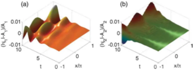
Numerical solutions of the ODE model(13)are presented in Fig. 1 for parameters corresponding to the BCS regime. It is found that amplitudes increase exponentially in time and the behavior agrees well with the theoretical predictions. Using the same parameters, we perform numerical simulations of the full partial differential equation (PDE) model (1) describing the Fermi-Bose mixture (see Fig.2). Results shows quantitative agreement for the PDE and ODE models up to
t∼10 [see the inset of Fig. 1(a)]. From Fig.3, where data for the spatial wavelengthLof the FW versus the modulation frequency are plotted [Fig.3(a)], it is seen how the wavelength decreases with increasing frequency. While results for the wave numberk=1 have been presented in Figs.1and2, we have numerically confirmed the results fork=2,3,4 also with full PDE simulations [squares in Fig.3(a)]. In Fig.3(b)we show howLdepends on the fermionic subsystem parameterκwithin the analytic model(18).
(a)
FIG. 1. (Color online) Solutions to the ODE model of Eq.(13). Blue dashed curves are forV (bosons) and red thin curves are for
Q (fermions). (a) Amplitudes growing exponentially in time. The inset shows a comparison with the corresponding PDE data (x=0 slices of Fig.2) for selected times. The PDE data are shown with black squares for bosons and dots for fermions. (b) Spectrum for the modulation frequency 12,+=65.5 for the wave numberk=1 (see
the text) and with 1and 2 from Eq.(9), which agrees well with Eq.(10)in this regime. The initial conditions areV /A1=Q/A2= 10−4(V
t=Qt =0) and the parameters areα12=0.25,A1= √
300,
A2= √
20,g(0)b =0.01,g
(0)
12 =0.8, andκ=1/4.
The results of Eq.(19)in practice here mean that with the parameter values of Fig.1, the modulation frequency can be on the order of 1% larger (or smaller) when exciting the FW. This is confirmed numerically with Eqs.(1)and(13); we have also observed a weak dependence on α12 for the maximum of the numerical 12 resonance region (not shown). Hence, by optimizing 12, a larger amplitude can be obtained (i.e., curve A in Fig.6can be moved further towards the line of the theoretical gain).
B. Driven nonlinearity in the bosonic subsystem The case where only the intraspecies (boson-boson) inter-action parameter is modulated is described by the system(14). Applying again the multiscale approach (see the Appendix), we have concluded that resonances occur at b =2ω1under
FIG. 2. (Color online) Solutions to the full PDE model of Eq.(1) for driven coupling between fermions and bosons with the modula-tion frequency 12,+=65.5 (k=1). We plot the oscillating parts
(|ψj| −Aj)/Ajfor (a)j=1 (bosons) and (b)j=2 (fermions). The
initial conditions areψj =Aj[1+10−4exp(ikx)] and the boundary
0 200 400 600 0
0.2 0.4 0.6 0.8
1 (a)
12,+
L/2
0 0.1 0.2 0.3
0 1 2 3
(b)
MI
12,+=135 a=b Larger A2
BCS Unitarity
L/2
FIG. 3. (Color online) Spatial wavelengths of the Faraday pat-terns. (a) We use the same parameters as for Fig.1with the left dot fork=1, corresponding to 12,+=65.5, and squares fork=2,3,4.
(b) The case corresponding to Fig.1(right dot) is the second (blue) curve from the bottom. Here, as well as for the lowest (red) curve [left square in (a)] where 12,+=135 (k=2), the condition(12)
is not fulfilled in the entire domain, hence MI is possible in the left part (dashed lines). The condition (12) for not having MI can be satisfied in the entireκrange, e.g., by choosingA2=2
√ 20 larger [top (green) curve]. Finally, the special case of a=b (i.e., with
gb(0)∝κ) is illustrated with the third (black) curve, where the left dot corresponds to the case illustrated in Fig.4.
the additional condition that ω1≃ω2. Hence, from Eq. (8) withω1=ω2we now obtain
b=2k
k2+a, k2 =a
2
1+ 2b/a2−1
. (21)
The corresponding instability region is bounded by the lines
¯
ω21 =ω21±ε0αb
2 , ω¯2 =ω¯1 (22) and the maximal gain is now equal to
pm≃
ε0αb
4ω1
. (23)
(a)
FIG. 4. (Color online) Solutions to the ODE model of Eq.(14). (a) Amplitudes growing exponentially in time. The inset shows a comparison with the corresponding PDE data (x=0 slices of Fig.5 for selected times): black squares are for bosons and dots for fermions. (b) Spectrum for the modulation frequency b=63.3 (k=1) and
with 1and 2agreeing well with Eq.(11)in this regime. The initial conditions are the same as in Fig.1; the parameters here areαb =0.25, A1=√5000,A2=√20.2,gb(0)=0.1,g
(0)
12 =0.8, andκ=1/16.
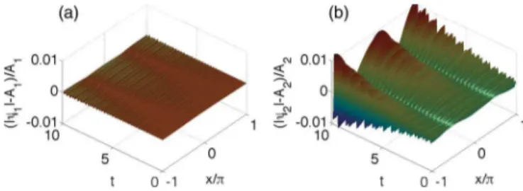
FIG. 5. (Color online) Solutions to the full PDE model of Eq. (1)for driven nonlinearity for bosons with the modulation frequency
b =63.3 (k=1). The initial and boundary conditions are the same
as in Fig.2; the parameters are the same as in Fig.4.
Numerical solutions of the ODE model(14)with exponen-tially growing amplitudes are presented in Fig.4for parameters corresponding to the molecular unitarity limit. In the spectrum we can see peaks corresponding to the combination of two excited frequencies for both components. These predictions are again well confirmed by PDE simulations (Fig.5) of the system(1) with driven nonlinearity of bosons [see the inset of Fig.4(a)]. Although the bosonic componentψ1is lagging behind (i.e., lower amplitude in Figs.4and5) it is growing exponentially with the same rate asψ2.
According to Eq.(22), the modulation frequency can be on the order of 3% larger or smaller (for the parameters of Fig.4) when exciting the FW. This has been confirmed numerically with Eqs.(1)and(14), although the maximum of the numerical resonance region (not shown) was found for slightly lower values of b than the theoretical estimate. Hence this means
that curve B in Fig.6can be made steeper by using slightly lower values for b.
Finally, we can analyze also this case in terms of the symmetric (or antisymmetric) combinationsξ±. From Eq.(14) we then have the driven coupled Mathieu-like system
ξ±,t t + 21,2ξ±+αbω21cos( bt)[ξ++ξ−]/2=0, (24)
and in agreement with our findings above, the literature here states that b≃2 1,2 2, and 1+ 2[12,37].
0 0.5 1 1.5 2
0 2 4 6
A B
C
α j
p
FIG. 6. (Color online) Exponential growth ratespof the slowly varying amplitudes [envelope ofV ∼Q∼exp(pt) of Eq.(7)]. Solid curves connect numerical data points (circles) for the three cases: A (Fermi-Bose modulationαj=α12), B (Bose-Bose modulationαj= αb), and C (super-resonanceαj =αb= −α12). Dashed lines shows
theoretical predictions according to Eq.(20)for case A and Eq.(23) for case B. In case A, 12=65.5, while in cases B (C) we use
C. Driven super-resonance
In the case of super-resonance we refer to the situation where both Bose-Bose time-modulated interactions [αb =0 in
Eq.(2)] and Fermi-Bose time-modulated interactions (α12 = 0) are simultaneously present in Eqs.(1)and(7). Comparing Eq. (16) with Eq.(21), we note that when a=b, we have 12,+= b. Now we change a sign in Eq.(2)such that for
α12 = −αb, for example, the two types of modulations initiate
opposite phases for the two components and an increased growth rate of the Faraday waves is observed, as compared to the two distinct cases discussed before. To demonstrate the super-resonance numerically we used the same parameters as for Fig.4withα12= −0.25. This result can also be understood from a consideration of the system (7) for symmetric and antisymmetric combinationsξ+ andξ−. For example, in the case whenα12 = −αb/2 and 12 = b, we simply have the
driven coupled Mathieu-like system
ξ±,t t+
2
1,2+ 22,1
αb
2 cos( bt)
ξ±
= −ω21αb
2 cos( bt)ξ∓. (25)
V. GROWTH OF THE FARADAY WAVES
In general we note that in the regime where the linear stability analysis based on Eqs. (5) and (6) is valid we have quantitative agreement between the full model(1)(see Figs. 2 and 5) and the ODE models (13) and(14) (Figs. 1 and4, respectively). We found an exponential growth in time of the oscillating amplitudes in this regime. For larger times the nonlinearities of the full model(1)cause a saturation of the amplitudes, while the results of the linear stability analysis become unphysical.
In Fig. 6 we show results of the exponential growth rate for Secs.IV A–IV Ctogether with the theoretical results for the maximal gain derived in the Appendix. We show results only for the wave numberk=1; however, we note that the theoretical estimatespm(k) increase withkand asymptotically
approach the constant limk→∞pm(k)=αjg(0)12A1A2/2.
VI. REALISTIC PARAMETERS
The Faraday waves can be observed, for example, in mixtures such as41K-40K and87Rb-40K [38]. Here we estimate effective values for the first system above since the two atomic masses are almost equal then. The fermion-boson scattering length a12 can be tuned by using the Feshbach resonance techniques according to [24]
a12 =abg
1+ B
B(t)−B0
,
whereB≃53 G,B0≃541.5 G, andabg≃65a0(abgis the background atomic scattering length anda0the Bohr radius). By variations in time of the external magnetic fieldB(t) around
B0, we can tune the scattering lengtha12. For example, we takea12=250a0andab =85a0and assume a length scale in the trap ofl=2.3μm. If we then consider the BCS regime (κ=1/4) and take the numbers of bosons and fermions as
Nb=2×10⁵ and Nf =2×10³, with the transverse trap
frequency beingω⊥=1.9 kHz, we find that for modulations with the frequency 12 ≃32ω⊥ the spatial wavelength of
the Faraday pattern is L≈31 μm. Correspondingly, in the molecular unitarity limit (κ =1/16) the spatial wavelength is
L≈16μm.
VII. CONCLUSION
We have illustrated the possibility of Faraday patterns for Fermi-Bose mixtures, i.e., with atomic bosons coupled to fermions, in both the fermionic BCS regime and the molecular unitarity limit. In particular we have investigated quasi-one-dimensional superfluid FB mixtures with periodic variations in time of the Fermi-Bose or Bose-Bose interactions. We find Faraday patterns for both cases and study their properties depending on the parameters for modulations and the system settings. Combining the two types of modulations can result in even larger amplitudes. We also conjecture that Faraday waves can be observed in an atomic BEC coupled to a Tonks-Girardeau gas.
A natural continuation of this work is to investigate Faraday patterns in FB mixtures for the two- and three-dimensional cases. This problem deserves a separate investigation though, since the corresponding coupled nonlinear Schr¨odinger-like equations are different.
ACKNOWLEDGMENTS
F.Kh.A. acknowledges partial support from the Fundac¸˜ao de Amparo `a Pesquisa do Estado de S˜ao Paulo, Brazil, and through the Otto Mønsted Guest Professorship at DTU.
APPENDIX
To understand the resonances in the coupled system(13), we can use the multiscale analysis [35]. Following this approach, we look for solutions where
ω21 =ω012 +ε0a1+ε02a2+ · · ·,
(A1)
ω22 =ω022 +ε0b1+ε02b2+ · · ·
and correspondingly for the functionsV andQ,
V =V0(t,T)+ε0V1(t,T)+ε20V2(t,T)+ · · ·, (A2)
Q=Q0(t,T)+ε0Q1(t,T)+ε20Q2(t,T)+ · · ·, whereT =ε0tis a slow time. Taking the terms of each order in
ε0, we obtain from Eq.(13)the following system of equations up to the linear order inε0:
V0,t t+ω201V0=0, Q0,t t+ω202Q0=0,
V1,t t+ω201V1= −2V0,t T −a1V0+[1+α12cos( t)]Q0,
Q1,t t+ω202Q1= −2Q0,t T −b1Q0+[1+α12cos( t)]V0. (A3) The solutions of the first two uncoupled equations of Eqs.(A3) can be written in the form
V0(t,T)=A0(T) cos(ω01t)+B0(T) sin(ω01t), (A4)
We require the absence of the resonant terms on the right-hand sides of the third and fourth of Eqs.(A3). With the ansatz =ω2±ω1and after averaging in the fast timet, we obtain a system of equations for the envelope functionsA0,B0,C0, andD0of Eqs.(A4),
2ω01A0,T −a1B0∓
α12
2 D0=0, −2ω01B0,T −a1A0+
α12
2 C0=0,
(A5) 2ω02C0,T −b1D0∓
α12
2 B0=0, −2ω02D0,T −b1C0+
α12
2 A0=0.
Looking for solutions of the form A0,B0,C0,D0∼exp(pt), i.e., for example, with A0,T ∼pA0/ε0, we find from Eqs.(A5)the characteristic equationp4+Mp2+N =0 with coefficients
M= 2b
2
1ω201+2a12ω202∓α212ω01ω02 8ω201ω202 ,
(A6)
N =
4a1b1−α122
2
256ω201ω202 .
Remember that the sign∓inMof Eqs.(A6)is for 12,±=
ω2±ω1, respectively, and note also thatN 0. Hence, from
p2= −M/2±M2/4−N it is seen that only
12,+ can
correspond to a positive realp, i.e., a FW with an exponentially growing amplitude, while excitations for 12,−are stable. The
maximal exponential growth rate of the FW for 12,+is found
from Eqs.(A6)withM2∼4N to be
pm∼
−M 2 ≃
ε0α12 4√ω1ω2
, (A7)
which is referred to as the theoretical gain in the main text.
For experiments on FW it is important to know also the width of the instability region. The boundaries of the unstable region can be found from inspection of Eqs. (A6), which shows that at the boundary we have fromNthatb1 =α212/4a1 and correspondingly fromMwe then havea1 = ±α212√ω1/ω2 such that the frequencies to linear order inε0 obtained from
Eqs.(A1)are
ω21 =ω201±ε0
α12 2
ω
1
ω2 + · · ·
,
(A8)
ω22 =ω202±ε0
α12 2
ω
2
ω1 + · · ·
.
Analogously the system(14)for the case of driven boson-boson interactions can be investigated and the results are reported in Eqs. (21)–(23). Below we sketch the derivation also for this case.
Forε0=0 the first of Eqs.(14)is a Mathieu equation
Vt t+
ω21+αbω21cos( t)
V =0, (A9) with solutions V =ACe(a,q,t)+BSe(a,q,t), where a=
4ω21/ 2andq = −2αbω12/ 2in the standard notation of the
cosine and sine Mathieu functions [36]. We now look again for solutions to Eqs.(14)of the form of Eqs.(A1)and(A2). In the case ofαb ≪1 one can use the expansions Ce(a,q,t)∼
cos(ω01t)+O(q) and Se(a,q,t)∼sin(ω01t)+O(q) in Eq. (A9). In particular we then have that the system in the first two of Eqs.(A3), and hence Eqs.(A4), applies also here and we have in the linear order
V1,t t+ω201V1 = −2V0,t T −a1V0−αbcos( t)V0+ε0Q0,
Q1,t t +ω022 Q1 = −2Q0,t T −b1Q0+ε0V0. (A10) HenceA0andB0are not coupled toC0andD0in the lowest order inε0such that it is enough to consider the two envelope functionsA0 andB0 in the remainder. We then require the absence of the resonant terms on the right-hand side of the first of Eqs. (A10). With the ansatz =2ω1 andω2=ω1 (b1 =a1), we obtain a system of equations forA0(withA0,T ∼
pA0/ε0) andB0such that the characteristic equations give
p= ± ε0
2ω1
α2
b
4 −a 2
1. (A11)
Hence the theoretical gain fora1∼0 is
pm=
ε0αb
4ω1
. (A12)
Since p becomes imaginary when a12> α2b/4, we have the boundarya1 =b1= ±αb/2 and henceω12=ω22≃ω012 ±
ε0α2b.
[1] M. Faraday, Philos. Trans. R. Soc. London 121, 319 (1831).
[2] F. Matera, A. Mecozzi, M. Romagnoli, and M. Settembre,Opt. Lett.18, 1499 (1993).
[3] F. Kh. Abdullaev, Pis’ma Zh. Tekh. Fiz.20, 25 (1994). [4] F. Kh. Abdullaev, S. A. Darmanyan, S. Bishoff, and M. P.
Sørensen,J. Opt. Soc. Am. B14, 27 (1997).
[5] F. Kh. Abdullaev, S. A. Darmanyan, and J. Garnier, Prog. Opt. 44, 306 (2002).
[6] A. Armaroli and F. Biancalana,Opt. Express20, 25096 (2012). [7] M. Droques et al., CLEO: Science and Innovations (OSA,
Washington, DC, 2012), p. CTh4B.7.
[8] K. Staliunas, S. Longhi, and G. J. de Valc´arcel,Phys. Rev. Lett. 89, 210406 (2002).
[9] K. Staliunas, S. Longhi, and G. J. de Valc´arcel,Phys. Rev. A70, 011601 (2004).
[10] M. Modugno, C. Tozzo, and F. Dalfovo, Phys. Rev. A 74, 061601(R) (2006).
[11] A. I. Nicolin, R. Carretero-Gonzalez, and P. G. Kevrekidis,Phys. Rev. A76, 063609 (2007);A. I. Nicolin,Phys. Rev. E84, 056202 (2011);Rom. Rep. Phys.63, 1329 (2011).
[12] A. B. Bhattacherjee,Phys. Scr.78, 045009 (2008).
[15] K. Lakomy, R. Nath, and L. Santos,Phys. Rev. A86, 023620 (2012).
[16] M. Kr¨amer, C. Tozzo, and F. Dalfovo,Phys. Rev. A71, 061602 (2005);C. Tozzo, M. Kr¨amer, and F. Dalfovo,ibid.72, 023613 (2005).
[17] D. Kobyakov, V. Bychkov, E. Lundh, A. Bezett, and M. Marklund,Phys. Rev. A86, 023614 (2012).
[18] P. Engels, C. Atherton, and M. A. Hoefer,Phys. Rev. Lett.98, 095301 (2007).
[19] P. Capuzzi and P. Vignolo,Phys. Rev. A78, 043613 (2008). [20] R. A. Tang, H. C. Li, and J. K. Hue,J. Phys. B44, 115303
(2011).
[21] Yu. Kagan, E. L. Surkov, and G. V. Shlyapnikov,Phys. Rev. A 54, R1753 (1996).
[22] Yu. Kagan and L. A. Manakova,Phys. Rev. A76, 023601 (2007). [23] S. Inouye, M. R. Andrews, J. Stenger, H.-J. Miesner, D. M. Stamper-Kurn, and W. Ketterle, Nature (London) 392, 151 (1998).
[24] H. Saito and M. Ueda, Phys. Rev. Lett. 90, 040403 (2003); F. Kh. Abdullaev, A. M. Kamchatnov, V. V. Konotop, and V. A. Brazhnyi, ibid. 90, 230402 (2003); D. E. Pelinovsky, P. G. Kevrekidis, and D. J. Frantzeskakis, ibid. 91, 240201 (2003);F. Kh. Abdullaev, J. G. Caputo, R. A. Kraenkel, and B. A. Malomed,Phys. Rev. A67, 013605 (2003).
[25] P. Capuzzi, M. Gattobigio, and P. Vignolo,Phys. Rev. A 83, 013603 (2011).
[26] S. K. Adhikari and L. Salasnich,Phys. Rev. A76, 023612 (2007); 77, 033618 (2008); 78, 043616 (2008).
[27] L. Tonks, Phys. Rev.50, 955 (1936);M. Girardeau,J. Math. Phys. (NY)1, 516 (1960).
[28] E. B. Kolomeisky, T. J. Newman, J. P. Straley, and X. Qi,Phys. Rev. Lett.85, 1146 (2000);M. ¨Ogren, G. M. Kavoulakis, and A. D. Jackson,Phys. Rev. A72, 021603(R) (2005).
[29] H. Heiselberg, Phys. Rev. Lett. 93, 040402 (2004); 108, 249904(E) (2012).
[30] A. Bulgac and G. F. Bertsch, Phys. Rev. Lett. 94, 070401 (2005).
[31] N. Manini and L. Salasnich,Phys. Rev. A71, 033625 (2005). [32] G. E. Astrakharchik, R. Combescot, X. Leyronas, and
S. Stringari, Phys. Rev. Lett. 95, 030404 (2005); G. E. Astrakharchik, J. Boronat, J. Casulleras, and S. Giorgini,ibid. 93, 200404 (2004).
[33] S. K. Adhikari,Phys. Rev. A77, 045602 (2008).
[34] A. H. Nayfeh,Introduction to Perturbation Techniques (Wiley-VCH, Weinheim, 1981), p. 253.
[35] G. M. Makhmoud,Physica A242, 239 (1997).
[36] M. Abramowitz and I. A. Stegun,Handbook of Mathematical Functions with Formulas, Graphs, and Mathematical Tables (Dover, New York, 1972).
[37] J. Hansen,Ing. Arch.55, 463 (1985).