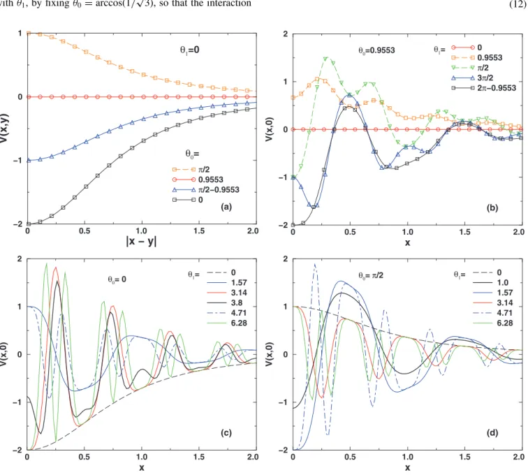
Bright solitons in quasi-one-dimensional dipolar condensates with spatially modulated interactions

Ao Dr Oliver Duenisch pelos contatos feitos e orientação de língua estrangeira Ao Dr Agenor Maccari pela ajuda na viabilização da área do experimento de campo Ao Dr Rudi Arno

Neste trabalho o objetivo central foi a ampliação e adequação do procedimento e programa computacional baseado no programa comercial MSC.PATRAN, para a geração automática de modelos

Ousasse apontar algumas hipóteses para a solução desse problema público a partir do exposto dos autores usados como base para fundamentação teórica, da análise dos dados

In an earlier work 关16兴, restricted to the zero surface tension limit, and which completely ignored the effects of viscous and magnetic stresses, we have found theoretical

The irregular pisoids from Perlova cave have rough outer surface, no nuclei, subtle and irregular lamination and no corrosional surfaces in their internal structure (Figure

Extinction with social support is blocked by the protein synthesis inhibitors anisomycin and rapamycin and by the inhibitor of gene expression 5,6-dichloro-1- β-

Peça de mão de alta rotação pneumática com sistema Push Button (botão para remoção de broca), podendo apresentar passagem dupla de ar e acoplamento para engate rápido

Vale destacar que, a princípio, o pesquisador poderia se deixar conduzir pela resposta cinco ou, ainda, se não estivesse mediando esse processo, não teria notado