Wald tests for IV regression with weak instruments

FUNDAÇÃO GETÚLIO VARGAS

ESCOLA de PÓS-GRADUAÇÃO em ECONOMIA

Lucas Pimentel Vilela

Wald tests for IV Regression with

Weak Instruments

Lucas Pimentel Vilela

Wald tests for IV Regression with

Weak Instruments

Dissertação para obtenção do grau de mestre apresentada à Escola de Pós-Graduação em Economia

Área de concentração: Econometria

Orientador: Marcelo J. Moreira

Ficha catalográfica elaborada pela Biblioteca Mario Henrique Simonsen/FGV

Vilela, Lucas Pimentel

Wald tests for IV regression with weak instruments / Lucas Pimentel Vilela. –

2013. 44 f.

Dissertação (mestrado) - Fundação Getulio Vargas, Escola de Pós-Graduação em Economia.

Orientador: Marcelo J. Moreira. Inclui bibliografia.

1. Variáveis instrumentais (Estatística). 2. Análise de regressão. 3. Testes de hipóteses estatísticas. I. Moreira, Marcelo J. II. Fundação Getulio Vargas. Escola de Pós-Graduação em Economia. III. Título.

Acknowledgements

Resumo

Esta dissertação trata do problema de inferência na presença de identi…cação fraca em modelos de regressão com variáveis instrumentais. Mais especi…camente em testes de hipóteses com relação ao parâmetro da variável endógena quando os instrumentos são fracos. O principal foco é nos testes condicionais unilaterais baseados nas estatísticas de razão de máxima verossimilhança, score e Wald. Resultados téoricos e numéricos mostram que o teste t condicional unilateral baseado no estimador de mínimos quadrados em dois estágios tem uma boa performance mesmo na presença de instrumentos fracamente correlacionados com a variável endógena. A abordagem condicional corrige uniformemente o tamanho do teste t e quando a estatística F populacional é tão pequena quanto dois, o poder do teste é proximo ao power envelope tanto de testes similares quanto de não similares. Tal resultado é surpreendente visto a má performace dos testes t’s condicionais bilaterais relatada em (6, Andrews, Moreira and Stock (2007)). Dado esse resultado aparentemente contra intuitivo, apresentamos novos testes t’s condicionals bilaterais que são aproximadamente não viesados e performam, em alguns casos, tão bem quanto o teste condicional baseado na estatística de razão de verossimilhança de (19, Moreira (2003)).

Abstract

This dissertation deals with the problem of making inference when there is weak identi…cation in models of instrumental variables regression. More speci…cally we are interested in one-sided hypothesis testing for the coe¢cient of the endogenous variable when the instruments are weak. The focus is on the conditional tests based on likelihood ratio, score and Wald statistics. Theor-etical and numerical work shows that the conditional t-test based on the two-stage least square (2SLS) estimator performs well even when instruments are weakly correlated with the endo-genous variable.The conditional approach correct uniformly its size and when the population F-statistic is as small as two, its power is near the power envelopes for similar and non-similar tests. This …nding is surprising considering the bad performance of the two-sided conditional t-tests found in (6, Andrews, Moreira and Stock (2007)). Given this counter intuitive result, we propose novel two-sided t-tests which are approximately unbiased and can perform as well as the conditional likelihood ratio (CLR) test of (19, Moreira (2003)).

List of Figures

7.1 Power curves for the one-sided conditional tests when _nk= 1. . . 28

7.2 Power curves for the one-sided conditional tests when nk= 2. . . 28

8.1 Null conditional distribution of t(k) when ln(qT=k) = 4. . . 30

8.2 Null conditional distribution of t(k) when ln(qT=k) = 1. . . 31

8.3 Null conditional distribution of t0(k) when ln(qT=k) = 4. . . 32

Contents

1 Introduction1 ₁₀

2 Model and Su¢cient Statistics 12

3 Invariant Similar Tests 14

4 Power Envelopes 17

4.1 Similar Power Envelope . . . 17 4.2 Non-Similar Power Envelope . . . 19

5 Weak IV Asymptotics 21

5.1 Tests for Unknown and Possibly Non-normal Errors . . . 21 5.2 Weak IV Asymptotic Results . . . 22

6 Strong IV Asymptotics 24

6.1 Local Alternatives . . . 24 6.2 Fixed Alternatives . . . 25

7 Numerical Results 27

8 Two-Sided Tests 30

I Appendix 34

Chapter 1

Introduction

1

Instrumental variables (IVs) are commonly used to make inferences about the coe¢cient of an endogenous regressor in a structural equation. When instruments are strongly correlated with the regressor, the tests based on the score (also known as lagrange multiplier (LM)), likelihood ratio (LR) and Wald (t-statistics) are asymptotically equivalent. This trinity of tests provides reliable inference as long as the instruments are strong. However, when identi…cation is weak, the three approaches are no longer comparable. (16, Kleibergen (2002)) and (18, Moreira (2002)) show that the LM statistic has a standard chi-square distribution regardless of the strength of the instruments. (19, Moreira (2003)) proposes a conditional likelihood ratio (CLR) test which is shown by (4, Andrews, Moreira and Stock (2006)) (hereinafter, AMS06a) to be nearly optimal. However, most results in the literature on the performance of tests based on the commonly used t-statistics are negative: (13, Dufour (1997)) shows that standard tests based on t-statistics can have size arbitrarily close to one; (6, Andrews, Moreira and Stock (2007)) (hereinafter, AMS07) …nd that conditional t-tests are severely biased; and (2, Andrews and Guggenberger (2010)) prove that subsampling tests based on the two-stage least squares (2SLS) t-statistic do not have correct asymptotic size. See (22, Stock, Wright, and Yogo (2002)), (14, Dufour (2003)), and (8, Andrews and Stock (2007)) for surveys on weak IVs.

In this dissertation we present one-sided conditional t-tests for testing the null hypothesis H0 : = 0 (or the augmented null H0 : 0) against the alternative H1 : > 0 (the

adjustment for H1 : < 0 is straightforward). We consider t-statistics centered around the

2SLS, the limited information maximum likelihood (LIML), the bias-adjusted 2SLS (B2SLS) and the estimator proposed by (15, Fuller (1977)) (Fuller’s estimator). We also introduce conditional tests based on an one-sided score (LM1) statistic, a likelihood ratio (LR1) statistic forH0: = 0, and a likelihood ratio statistic (MLR1) for H0 : 0. We develop a theory of optimal

tests for one-sided alternatives that parallels the two-sided results of AMS06a. We adopt the same invariance condition as in AMS06a and (11, Chamberlain (2007)) under which inference is unchanged if the IVs are transformed by an orthogonal matrix, e.g., by changing the order in which the IVs appear. We develop the Gaussian power envelope for point-optimal invariant similar (POIS) tests. When the null hypothesis is H0 : = 0, the conditional LR1 (CLR1)

test is nearly optimal in the sense that its power function is numerically close to the power envelope. For the more relevant nullH0 : 0, the CLR1 test does not control size uniformly.

The conditional t-tests have correct size and the one based on the 2SLS estimator numerically outperforms the conditional MLR1 (CMLR1) test. The LM1 test is a POIS test and does not have good power overall.

The good performance of the one-sided conditional 2SLS t-test is somewhat surprising con-sidering the bad performance of two-sided conditional t-tests found in AMS07. We show that the bad performance is due to the asymmetric distribution of t-statistics under the nullH0 : = 0

11

based on t-statistics. First, we propose novel tests which are by construction approximately unbiased. Second, we modify the t-statistics so that their null distribution is nearly symmetric. Both methods yield some t-tests whose power is close to the CLR test. Hence, this dissertation restores the triad of tests based on score, likelihood ratio, and t-statistics with reasonably good performance even when instruments are weak for two-sided hypothesis testing. By inverting the conditional t-tests, we can obtain informative con…dence regions around di¤erent estimators –including the commonly used 2SLS estimator.

The foregoing results are developed under the assumption of normal reduced-form errors with known covariance matrix. The …nite-sample theory is extended to non-normal errors with unknown variance at the cost of introducing asymptotic approximations. Under weak instru-mental variable (WIV) asymptotics, the exact distributional results extend in large samples to feasible versions of the proposed tests. The …nite-sample Gaussian power envelopes are also the asymptotic Gaussian power envelopes with unknown covariance matrix. Under strong-IV asymptotics, we derive consistency even when errors are nonnormal and asymptotic e¢ciency (AE) when errors are normal.2

The dissertation is organized as follows: Chapter2 introduces the model with one endogen-ous regressor variable, multiple exogenendogen-ous regressor variables, and multiple IVs. This chapter determines su¢cient statistics for this model with normal errors and reduced-form covariance matrix. Chapter3 introduces one-sided invariant similar tests. Chapter 4 …nds the power en-velope for similar and nonsimilar one-sided tests. Chapter 5 adjusts the tests to allow for an estimated error covariance matrix and analyzes their asymptotic properties under weak IVs. Chapter 6 obtains consistency and asymptotic e¢ciency for one-sided tests. Chapter 7 com-pares numerically the power of the tests considered in earlier chapters under WIV asympotics. Chapter8introduces novel unbiased two-sided tests. An appendix contains proofs of the results. The supplement presents: power comparisons for di¤erent one-sided and two-sided tests; similar and non-similar power envelopes which are numerically very close (this fact further strengthens our optimality results); and con…dence intervals for returns to schooling using the data of (9, Angrist and Krueger (1991)).

Chapter 2

Model and Su¢cient Statistics

In this dissertation we study linear instrumental variable regression models with the objective of making inference about the coe¢cient of the endogenous variable when the instruments are possibly weak. More speci…cally, we want to make hypothesis tests of in the following linear model:

y1 = y2 +X 1+u;

y2 = Ze +X 1+v2; (2.1)

wherey1; y2 2Rn; X 2Rn p;and Ze2Rn k are observed variables; u; v2 2Rn are unobserved

errors (possibily correlated); and 2R; ₁; _12Rp_{;and 2R}k _{are unknown parameters. The}

matrices X and Ze are taken to be …xed (i.e., non-stochastic) and Z = [X :Ze]has full column

rankp+k.

In the …rst and main part of this dissertation we are interested with one-sided hypothesis testing of the coe¢cient :1

H0 : = 0( orH0 : 0) against H1 : > 0 (2.2)

and in the last chapter we revise and deal with the two-sided hypothesis testing problem:

H0 : = 0 against H1 : 6= 0 (2.3)

It is convenient to transform the IV matrix Ze into a matrix Z which is orthogonal to X: Z0X= 0. Since we are interested only in , we can decompose the IV matrix Ze=Z+PXZe=

MXZe+PXZe, where MA= I PA and PA = A(A0A) 1A0 for any full column matrix A, and

work with the model:

y1 = y2 +X 1+u; (2.4)

y2 = Z +X +v2; (2.5)

where = ₁+ (X0X) 1X0Z :e

Furthermore, the model can be rewritten as a matricial reduced-form:

Y =Z a0+X +V; (2.6)

whereY = [y1:y2],V = [v1:v2] = [u+v2 :v2],a= ( ;1)0; = [ : ];and = 1+ :

The reduced-form errorsV are assumed to be independently and identically distributed (i.i.d) across rows. To obtain exact distribution of the tests, we assume that each row has a mean zero bivariate normal distribution withknown2 2nonsingular covariance matrix = [!ij]_i;j=1;2:As

13

shown below, the normality and the knowledge of assumptions can be relaxed when asymptotic approximations are considered.

The probability model for (2.6) is a member of the curved exponential family, and low dimensional su¢cient statistics are available. Lemma 1 of AMS06a shows that X0Y and Z0Y are independent and su¢cient for 0_; 0 0 _{and( ;} 0₎0_{, respectively. Since the assessment of the} performance of the tests is by its power we can focus only on tests based su¢cient statistics, in particular onZ0Y. As shown by (19, Moreira (2003)), we can apply a one-to-one transformation toZ0_{Y that yields thek 2 su¢cient statistic [S:T], where}2

S = (Z0Z) 1=2Z0Y b0 (b00 b0) 1=2 and

T = (Z0Z) 1=2Z0Y 1a0 (a00 1a0) 1=2; (2.7)

whereb0 = (1; 0)0 anda0 = ( 0;1)0:

The distribution of the su¢cient statistic[S:T]is multivariate normal,

vec[S:T] N(h ; I2k); (2.8)

with …rst moment depending on the following quantities:

h = (c ; d )0 _2R2 and = (Z0Z)1=2 _2Rk, (2.9)

wherec = ( ₀) (b0₀ b0) 1=2 and d =a0 1a0 (a00 1a0) 1=2:

Chapter 3

Invariant Similar Tests

Seems natural to suppose that our decision to reject or not the null hypothesis is invariant to changes in the coordinate system of the instrumental variables, i.e., the order in which each instrument appears, otherwise there is too much a priori information about the instruments and their relative relevance. The only exception to our knowledge that exclude speci…c in-struments and consequently depend on the order in which the inin-struments appears is given by (12, Donald and Newey (2001)). In consequence we restrict our analysis to tests that are invariant to orthogonal transformations, i.e., let be a[0;1]-valued statistic depending on the su¢cient statistics[S :T]andF be ak korthogonal matrix, so the tests considered are such

(F S; F T]) = (S; T).1

By Theorem 6.2.1 of (17, Lehmann and Romano (2005)) and Theorem 1 of AMS06a, a test is invariant if and only if it can be written as a function of

Q= [S:T]0[S:T] = S

0_{S S}0_T

T0S T0T =

QS QST

QST QT : (3.1)

The statisticQ has a Wishart distribution with rank one that depends on

(q) = h0qh =c2qS+ 2c d qST +d2qT; where

q = qS qST

qST qT 2R

2 2_{: (3.2)}

Note that (q) 0 because q is positive semi-de…nite almost surely (a.s.). De…ne Q1 =

(QS; QST). The density ofQ evaluated at(q1; qT) is given by

fQ1;QT(q1; qT; ; ) =K1exp( (c

2 _+d2_{)=2) det(q)}(k 3)=2 _(3.3)

exp( (qS+qT)=2)( (q)) (k 2)=4I(k 2)=2(

q

(q));

whereK1 is a constant, I ( ) denotes the modi…ed Bessel function of the …rst kind of order ,

and

= 0Z0Z 0: (3.4)

Examples of invariant test statistics are the (1, Anderson and Rubin (1949)) (AR), score and likelihood ratio statistics:

AR = QS=k;

LM = Q2_ST=QT;

LR = 1

2 QS QT + q

(QS QT)2+ 4Q2_ST : (3.5)

15

When the concentration parameter =(!22 k) is small, most test statistics are not

approxim-ately distributed normal or chi-square. For example, under the weak instrument asymptotics of (22, Staiger and Stock (1997) ) where =C=pn, theLRstatistic is not asymptotically pivotal. Its asymptotic distribution is nonstandard and depends on the nuisance and concentration para-meter =(!22 k) under the null. Consequently, the null rejection probability of the standard

likelihood ratio test depends on the concentration parameter.

(19, Moreira (2003)) proposes similar tests which reject the null hypothesis when the test statistic exceeds a critical value that depends on QT:

(QS; QST; QT)> ; (QT); (3.6)

where ; (qT) is the 1 quantile of the distribution of conditional on QT = qT when = ₀ :

P ₀( (QS; QST; QT))> ; (qT)) = ; (3.7)

In practice, the critical value function ; (QT)of the conditional test given in (3.6) is unknown

and must be approximated. Given a statistic (QS; QST; QT) write it as a function of QS, S2 = QST=(jjSjj jjTjj) and QT, by Lemma 3, (f) of AMS06a, (QS;S2) is independent of QT

and has a nuisance-parameter free distribution when = ₀. The null distribution of (QS;S2)

can be approximated by simulating nM C i.i.d random vectors Si N(0; Ik) for i = 1; :::;

nM C where nM C is large. The approximation to ; (QT) is the 1 sample quantile of f (S_i0Si; S_i0ek1 Q

1=2

T ; QT) :i= 1; :::; nM Cgand ek1 = (1;0; :::;0)0 2Rk.

We now introduce several new one-sided invariant similar tests for testing H0 : = 0 (or

H0 : 0) against H1 : > 0. Each similar test will reject the null hypothesis when the

one-sided statistic is larger than the critical value function ; .

The one-sided t-statistics are based on the k-class estimators of and its derivation are present in the appendix:2

t(k) = (k) 0

u(k)[f22QS+g22QT + 2f2g2QST n(k 1)w22] 1=2

, where

(k) = f1f2QS+g1g2QT + (g1f2+f1g2)QST n(k 1)w21

f₂2QS+g22QT + 2f2g2QST n(k 1)w22

,

2

u(k) = b(k)0 b(k) and b(k) = (1; (k))0, (3.8)

wherefl=b00 el= p

b0

0 b0,gl=a00el=

p

a0

0 1a0,e1 = (1;0)0 and e2 = (0;1)0 forl= 1;2.

Here we will use four k-class: the 2SLS estimator, the limited information maximum like-lihood for known (LIMLK) estimator, the bias-adjusted 2SLS (B2SLS) estimator and the Fuller’s estimator:

2SLS: k= 1;

LIMLK: k=kLIM LK = 1 + (QS LR)=n

B2SLS: k=n=(n k+ 2);

Fuller: k=kLIM LK 1=(n k p):

(3.9)

The …nite-sample properties of the estimators (k)depend onk. Consequently, the behavior of thet(k) statistics can be sensitive to the choice ofk.

We construct two statistics from the likelihood of the model given in (2.6) with known. The …rst one-sided statistic based on the standard LR statistic (i.e., 2 times the logarithm of

the likelihood ratio) is for testingH0: = 0:

LR1 = 2 "

sup 0

lc(Y; ; ) lc(Y; 0; )

#

=R( ₀) inf 0

R( ), where

R( ) = b

0_Y0_P

ZY b

b0 _b withb= (1; )

0_{; (3.10)}

16

andlc(Y; ; )is the log-likelihood function for known with all parameters concentrated out

except . In the Appendix, we show that R( ) and LR1 depend on the observations only throughQ and

LR1 =LR 1( (k_{LIM LK}) ₀) + max_f0; R( ₀) R(₁)_g 1( (k_{LIM LK})< ₀); (3.11)

whereR(₁) = lim !1R( ). We will see later in the numerical results that the power function P ; (LR1> LR1; (QT))is not monotonic for < 0. As a result, the CLR1 test will not have

correct size when the null hypothesis is H0 : 0.Given that, we present another one-sided

statistic based on the likelihood function: the modi…ed LR statistic for testingH0 : 0:

M LR1 = 2 "

suplc(Y; ; ) sup 0

lc(Y; ; ) #

= inf 0

R( ) R( (k_{LIM LK})): (3.12)

In the Appendix, we show that

M LR1 = [LR max_f0; R( ₀) R(₁)_g] 1( (k_{LIM LK}) ₀): (3.13)

Chapter 4

Power Envelopes

In this chapter, we address the question of optimal invariant similar and nonsimilar tests when the IV’s may be weak. To evaluate the performance of the novel one-sided conditional tests, we derive the power envelopes for similar and nonsimilar tests. The use of su¢ciency and invariance reduces the dimension of the parameters from1 +k+ 2pfor = ( ; 0; 0; 0)0to just2for( ; )0. The dimension reduction allows the power envelope to meaningfully assess the performance of our one-sided tests. The envelope we derive here consists of upper bound for power and lower bound for size for eitherH0 : = 0 orH0 : 0.

4.1

Similar Power Envelope

The following theorem is the main result of this section:

Theorem 1 De…ne the statistic

LR (Q1; QT) =

fQ1;QT(q1; qT; ; )

fQT(qT; ; )fQ1jQT(q1jqT; 0)

= '1(q1; qT; ; )

'₂(qT; ; )

; (4.1)

where

'₁(q1; qT; ; ) = exp( c2=2)( (q)) (k 2)=4I(k 2)=2

q

(q) and

'₂(qT; ; ) = d2qT (k 2)=4I(k 2)=2

q

d2qT : (4.2)

Let ; (QT) be a shorthand for LR ; (QT). Then the following hold:

(a) For ( ; ) with > ₀, the test that rejects H0 : = 0 when LR (Q1; QT) >

; (QT) maximizes power over all level invariant similar tests.

(b) For ( ; ) with < ₀, the test that rejects H0 : = 0 when LR (Q1; QT) <

;1 (QT) minimizes the null rejection probability over all level invariant similar tests.

Comments: 1. We denote the test that rejects the null when LR (Q1; QT) > ; (QT)

as a point-optimal invariant similar (POIS) test. We determine the power upper bound by considering the POIS tests for arbitrary values( ; ) when > ₀. The power upper bound is for similar tests forH0: = 0. We do not impose the additional constraint that tests must

have correct size, and so the upper bound could be conservative for H0 : 0. We shall see

later that even for small values of , some tests forH0 : 0 do reach the upper bound.

2. The test which rejects the null when LR (Q1; QT) < ;1 (QT) is called POIS0

test. We determine the null lower bound by …nding the power of POIS0 tests for arbitrary values

( ; ) when < ₀.

18

4. The denominator '₂(qT; ; ) does not depend on q1 and can be absorbed into the

conditional critical value. Thus, the test based onLR (Q1; QT) is equivalent to a test based

on the numerator of'₁(q1; qT; ; ). For reasons of numerical stability, however, we recommend

constructing critical values usingln(LR (Q1; QT)).

We now show that such tests do not depend on , so that the POIS and POIS0 tests are of a relatively simple form. Using a series expansion ofI(k 2)=2(x), we can write

'₁(q1; qT; ; ) = 2 (k 2)=2exp( c2=2)

1

X

j=0

( (q1; qT)=4)j

j! ((k 2)=2 +j+ 1): (4.3)

The term'₂(qT; ; ) can be written analogously.

The function'₁(q1; qT; ; ) is increasing in (q1; qT) 0: As a result, for a …xed value of

;say > ₀, the optimal test for …xed alternative rejects H0 : = 0 when

(Q1; QT)> ; (QT); (4.4)

where ; (QT) is a shorthand for ; (QT) as de…ned in (3.7). This POIS test is one-sided

because it directs power at a single point that is greater than the null value ₀. An analogous argument shows that the POIS0 test that minimizes rejection probabilities for …xed < ₀ rejectsH0 when

(Q1; QT)< ;1 (QT). (4.5)

Corollary 2 For > ₀, the POIS test based on (Q1; QT) is the uniformly most powerful

test among invariant similar tests against the alternative distributions indexed by _f( ; ) :

> 0_g. For < ₀, the POIS0 test based on (Q1; QT) uniformly minimizes the null

rejection probability among invariant similar tests against the alternative distributions indexed

by _f( ; ) : >0_g.

Comments: 1. Although the form of the POIS and POIS0 tests does not depend on , their power depends on the true value of . Hence, the power envelope depends on both parameters

and .

2. A test based on (Q1; QT) is equivalent to a test that rejects when

P OIS1 = QS+ S2 p

QS k p

2k+ 2 > ; (QT); where

= (2d =c )pQT,), (4.6)

and ; (QT) is a shorthand for P OIS1 ; (QT) de…ned in (3.7). This formulation of the test

is convenient because QS; S2; and QT are independent under = 0, which simpli…es the

calculation of critical values.

3. Provided !12 !22 0 6= 0; the quantityd is a linear function of and equals zero if

and only if = _AR;where

AR=

!11 !12 0

!12 !22 0

: (4.7)

In this case, = 0 andP OIS1 reduces to QS= p

2k;which is the AR statistic re-scaled. Hence, the AR test, usually conceived as a two-sided test, is one-sided POIS against the alternative

= _AR:

4. The POIS test for local to 0 with > 0 (i.e., the LMPI test) is the one-sided LM

test that rejectsH0 if

19

wherez is the 1 quantile of the standard normal distribution. Analogously, if is local to ₀ with < ₀;then the LMPI test rejectsH0 if QST=Q1_T=2 > z .

5. The sign of in (4.6) can change as changes even for values on the same side of the null hypothesis becaused is a linear function of :As a result, the form of the P OIS1

statistic (and the power envelope) changes dramatically as varies. The constant determines the weight put on the statistic _S2. The optimal value of for small values of > 0 has the

wrong sign for large values of and vice versa. This fact has adverse consequences for the overall one-sided power properties of POIS tests.

6. The optimal one-sided test for arbitrarily large rejectsH0 if

QS+ 2(det( )) 1=2( 0!22 !12)QST > 1; (QT) (4.9)

for 1; ( ) as de…ned in (3.7). Remarkably, the same test is the optimal one-sided test for

negative and arbitrarily large in absolute value for any . Consequently, the optimal two-sided test for _{j 0j}arbitrarily large is the test in (4.9).

Corollary2shows that the POIS test for an alternative( ; )depends only on . Because the true parameter is unknown, we could construct an empirical version of the standardized optimal statistic:

e_b =x0_bQx_b; (4.10)

where x_b = (c_b=_jjh_bjj; d_b=_jjh_bjj)0 _{and b is the maximum likelihood estimator of under H}

1 :

> ₀. The next theorem shows that the empirical POIS test is equivalent to those based on CLR1 test.

Theorem 3 The statisticse_b and LR1 are equivalent up to strictly increasing transformations

(possibly depending on QT). In particular,

P ; (eb > e_b; (QT)) =P ; (LR1> LR1; (QT)): (4.11)

Comment: This theorem and Comment 5 of Corollary 2indicate that the CLR1 test does not have correct size when the null hypothesis is H0 : 0 instead ofH0: = 0. See chapter 7

below for numerical simulations on size and power of the CLR1 test.

4.2

Non-Similar Power Envelope

Non-similar tests have null rejection probability below the signi…cance level for some values of the nuisance parameter . Due to the continuity of the power function, for such values of , the power of a non-similar test is less than the power of a similar test for alternatives close enough to the null hypothesis. However, for other values of , or for more distant alternatives, non-similar tests can have greater power than similar tests. For this reason, we also consider optimal invariant non-similar tests of the hypothesisH0 : = 0 against point alternatives.

Our construction of point-optimal invariant (POI) non-similar tests follows Section 3.8 of (17, Lehmann and Romano (2005)). Consider the composite null hypothesis

H0: ( ; )2 f( 0; ) : 0 <1g; (4.12)

and the point alternative

H1 : ( ; ) = ( ; ): (4.13)

Let be a probability measure over_f : 0 <_1gand h be the weighted pdf,

h (q) = Z

20

where fQ1;QT(q1; qT; ; ) is given in (3.3). The e¤ect of weighting by under the null is

to turn the composite null into a point null, so that the most powerful test can be obtained using the Neyman-Pearson Lemma. Speci…cally, let be the most powerful test of h against fQ1;QT(q1; qT; ; ), so that rejects the null when

N P (q) = fQ1;QT(q1; qT; ; )

h (q) > d ; ; (4.15)

whered ; is the critical value of the test, chosen so thatN P (q)rejects the null with probability

under the distributionh .

If the test has size for the null hypothesisH0 in (4.12), i.e.,

sup

0 <1

P ₀; (N P (Q)> d ; ) = ; (4.16)

then the test is most powerful for testing H0 against H1, and the distribution is least

favorable; cf. Thm. 3.8.1 and Cor. 3.8.1 of (17, Lehmann and Romano (2005)).

Given a distribution , condition (4.16) is easily checked numerically. What proves more computationally di¢cult is …nding the distribution that satis…es (4.16). In the numerical work we consider distributions that put point mass on some point 0. In this case, we have

N P = fQ1;QT(q1; qT; ; )

fQ1;QT(q1; qT; 0; 0)

: (4.17)

Let _R( ₀; 0; ; j ; ) be the rejection probability of the test based on the statistic in

(4.17) when the true values are and . The numerical problem is to …nd the value of 0 such

that the test has size . Denote this value of 0 by LF0 ; then LF0 solves

R( ₀; LF₀ ; ; _{j 0}; LF₀ ) = and

sup

0 <1R

( ₀; LF₀ ; ; _{j 0}; ) : (4.18)

If there is a LF

0 ( 0; ; ) that satis…es (4.18), then the test based on N P LF

0 is the POI

non-similar test.

The power upper bound for invariant non-similar tests is_R( ₀; LF₀ ( ₀; ; ); ; _j ; )

(an analogous argument yields a null lower bound). We …nd numerically that the power envelopes for similar and non-similar tests are essentially the same, up to numerical accuracy. The reason for this is twofold. On one hand, the conditional critical values for the POIS tests depend on qT only weakly in the range of qT that is most likely to occur under the alternative. Thus, the

Chapter 5

Weak IV Asymptotics

Here, we consider the same model and hypotheses as in chapter2, but with non-normal reduced-form errors with unknown covariance matrix. We show that the …nite-sample distribution of the tests and statistics holds asymptotically under the same high-level assumptions as in (21, Staiger and Stock (1997)). To model weak IV asymptotics and …xed alternatives (WIV-FA), we let be local to zero and the alternative be …xed, not local to the null value ₀:

Assumption WIV-FA. (a) =C=n1=2 for some non-stochastick-vector C: (b) is a …xed constant for alln 1:

(c)k is a …xed positive integer that does not depend onn:

We now specify the asymptotic behavior of the instruments, exogenous regressors, and reduced-form errors:

Assumption 1. n 1_Z0_{Z !p D for some positive de…nite(k+p) (k+p) matrixD.}

Assumption 2. n 1V0V _!p for some positive de…nite 2 2 matrix :

Assumption 3. n 1=2_vec(Z0_{V)!dN(0; ) for some positive de…nite2(k+p) 2(k+p)matrix}

;where vec( ) denotes the column by column vec operator.

Assumption 4. = D.

The quantities C; D; and are assumed to be unknown. (3, Andrews, Moreira and Stock (2004)) (hereinafter, AMS04) show that Assumptions 1-3 hold under general condi-tions. Assumption 4 holds under Assumptions 1-3 and homoskedasticity of the errors Vi, i.e.,

E(ViVi0jZi) =EViVi0 = a:s.

We now introduce tests that are suitable for (possibly) non-normal, homoskedastic, uncor-related errors with unknown covariance matrix. See AMS04 for tests and results for cases in which the errors are not homoskedastic or are correlated. For clarity of the asymptotics results, we writeS; T; Q; etc. of chapter2, asSn; Tn; Qn;etc.

5.1

Tests for Unknown

and Possibly Non-normal Errors

For feasible tests, when the reduced-form error covariance matrix is unknown, we need to estimate consistently and it is achieved by the estimator:1

b_n= (n k p) 1Vb0V ;b whereVb =MZ;XY =Y PZY PXY; (5.1)

see Lemma 1 of (5, Andrews, Moreira and Stock (2006,b)) (hereinafter, AMS06b).

1_{This de…nition of b}

nis suitable ifZ orX contains a vector of ones, as is usually the case. If not, then bn is

22

Given that, we can replace by b_n and obtain modi…ed versions of the statistics Sn; Tn;

QS;n; QST;n and QT;n :

b

Sn = (Z0Z) 1=2Z0Y b0 (b00bnb0) 1=2;

b

Tn = (Z0Z) 1=2Z0Ybn1a0 (a00bn1a0) 1=2,

b

QS;n = Sbn0Sbn,QbST;n =Sbn0Tbn and QbT;n=Tbn0Tbn (5.2)

The feasible one-sided statistics for unknown are derived in the appendix and we present here:

bt bk

n =

b(bk) ₀ bu(bk)[fb2

2QbS;n+gb22QbT;n+ 2fb2gb2QbST;n n(kb 1)wb22] 1=2

, where

b(bk) = fb1fb2QbS;n+bg1bg2QbT;n+ (bg1fb2+fb1bg2)QbST;n n(bk 1)wb21 b

f2

2QbS;n+bg22QbT;n+ 2fb2bg2QbST;n n(bk 1)wb22

, and

b2u bk = 1; b(kb) bn 1; b(bk)

0 .

where fbl = b00bnel= q

b0₀bnb0 and gbl = a00el= q

a0₀bn1a0 for l = 1;2, and the k’s for the four

k-class estimators are given by:

2SLS: bk= 1

LIML: bk=bkLIM L= 1 + (QbS;n dLRn)=(n k p)

B2SLS: bk=n=(n k+ 2)

Fuller: bk=bkLIM L 1=(n k p):

(5.3)

For all remaining test statistics, we just need to replaceQS; QST andQT by their analogues

in which is estimated by b_n. For example, the LRtest statistic for unknown is de…ned as in (3.5), but withQS; QST and QT replaced byQbS;n ,QbST;n andQbT;n. We denote the resulting

test statistic by dLRn. The analogue of LR1,M LR1 and LM1 are denoted by LRd1n, M LR\1n

andLM[1n, respectively.

The critical value function for each test statistic is simply ; (QbT;n), as de…ned in (3.7).

5.2

Weak IV Asymptotic Results

In this section we derive the limit distribution of each one-sided test present in the previous section. In particular, we show that all tests converges in distribution to their respective …nite sample distribution under normality.

Under Assumptions WIV-FA and 1-4, Lemma 4 of AMS06a shows that

(Sn; Tn)!d(S1; T1);

(Sbn;Tbn;bn) (Sn; Tn; )!p 0;

(Sbn;Tbn;bn)!d(S1; T1; ); (5.4)

whereS1 and T1 are independentk-vectors which are de…ned as follows:

vec(NZ) N(vec(DZCa0); DZ);

S1 = D_Z1=2NZb0 (b00 b0) 1=2 N(c D1_Z=2C; Ik),

T1 = DZ1=2NZ 1a0 (a00 1a0) 1=2 N(d DZ1=2C; Ik); where

DZ = D11 D12D221D21,

D = D11 D12

D21 D22 ; D112R

k k_{; D}

23

The matrixDZ is the probability limit of n 1Z0Z:Under H0 : = 0; S1 has mean zero, but T1 does not. Let

Q1 = [S1:T1]0[S1:T1];

QS;1 = S10 S1; QST;1=S10 T1; QT;1=T10 T1;

S2;1 = S10 T1=(jjS1jj jjT1jj); and

1 = C0DZC: (5.6)

By (5.5), we …nd that the …nite-sample distribution of(QS;1; QST;1; QT;1) is the same as that of(QS;n; QST;n; QT;n) with n replaced by 1. Then the asymptotic distribution of the feasible tests and statistics are the same as …nite-sample case:

Theorem 4 Under Assumptions WIV-FAand 1-4 withbk de…ned in (5.3)

(a) (i)(bt(bk)n; t(k1); (QbT;n))!d(t(k1); t(k1); (QT;1));

(ii)(LRd1n; LR1; (QbT;n))!d(LR1(Q1;1; QT;1); LR1; (QT;1));

(iii)(M LR\1n; M LR1; (QbT;n))!d(M LR1(Q1;1; QT;1); M LR1; (QT;1)) (iv)(LM[1n; LM1; (QbT;n))!d(LM1(Q1;1; QT;1); LM1; (QT;1)) (b) (i)P(bt(bk)n> t(k1); (QbT;n))!P(t(k1)> t(k1); (QT;1));

(ii)P(LRd1n> LR1; (QbT;n))!P(LR1(Q1;1; QT;1)> LR1; (QT;1)),

(iii) P(M LR\1n> M LR1; (QbT;n))!P(M LR1(Q1;1; QT;1)> M LR1; (QT;1)); (iv) P(LM[1n> LM1; (QbT;n))!P(LM1(Q1;1; QT;1)> LM1; (QT;1));

(c)P(t(k1)> t(k1); (QT;1)) =P(LR1(Q1;1; QT;1)> LR1; (QT;1)) =P(M LR1(Q1;1; QT;1)>

M LR1; (QT;1)) =P(LM1(Q1;1; QT;1)> LM1; (QT;1)) = under = 0.

Comments. 1. The k0

1s are the limiting distribution of the statistics k and for all the four k-class considered k1 = 1. And the t-statistics t(k1) are the limiting distribution of t(k)n,

which are functions ofQ1 given in (5.6).

2. Part (c) asserts that conditional tests derived from the LRd1nand M LR\1n statistics and

Chapter 6

Strong IV Asymptotics

Two important large sample properties of tests arepointwise consistency: for a …xed alternative, the power of the test goes to one as the sample size increases; and asymptotic e¢ciency (AE): the test uniformly maximize the asymptotic power among the asymptotically unbiased tests (see (17, Lehmann and Romano (2005))). Given that, we analyze the asymptotic properties of the conditional tests based onLM[1n,LRd1n,M LR\1n, andbt(bk)nstatistics for both local alternatives

(SIV-LA) and …xed alternatives (SIV-FA). Under SIV-LA, we establish AE for the one-sided tests and under SIV-FA, we address consistency.

Before analyzing the asymptotic properties of the one-sided conditional tests, we need to establish the limit behaviour of the critical value functions under SIV-LA and SIV-FA. Under both asymptotics, SIV-LA and SIV-FA, QT;n diverges in probability to 1 as the sample size

increases. Given that we provide the following preliminary results:

Lemma 5 Let z be the 1 quantile of the standard normal distribution. As qT !p1,

(a)for anyk in (3.9), _t(k); (qT)!z ,

(b)for ₂(0;1=2), LR1; (qT)!z .

(c)for ₂(0;1=2), M LR1; (qT)!z .

Comment. As the sample size increases the statistic QT;n diverges to in…nity in probability

which implies, by the previous result, that the critical value functions of the tests considered converge in probability to the1 quantile of the standard normal distribution.

6.1

Local Alternatives

For local alternatives, is local to the null value 0 as the sample size increases:

Assumption SIV-LA. (a) = ₀+B=n1=2 for some constantB >0: (b) is a …xed non-zerok-vector for alln 1:

(c)k is a …xed positive integer that does not depend onn:

We use Lemma 6 of AMS06a to establish the strong IV-local alternative limiting distribution of tests. Under Assumptions SIV-LA and 1-4:

(Sn; Tn=n1=2)!d(SB1; T); (6.1) (Sbn;Tbn=n1=2;bn) (Sn; Tn=n1=2; )!p 0;

(Sbn;Tbn=n1=2;bn)!d(SB1; T; );

whereSB1 and T arek-vectors de…ned as follows:

SB1 N( S; Ik); where (6.2)

S = D_Z1=2 B(b00 b0) 1=2 and

25

These de…nitions allow us to determine the behavior of theLM[1n,LRd1n,M LR\1n, andbt(bk)n

statistics under SIV-LA asymptotics.

Theorem 6 Under Assumptions SIV-LA and 1-4 withbk de…ned in (5.3):

(a)bt(bk) =t(k) +op(1)!d( 0_TSB1)=jj Tjj.

(b)LM[1n=LM1n+op(1)!d( 0TSB1)=jj Tjj,

(c)LRd11_n=2=LR11n=2+op(1)!dmaxf( 0TSB1)=jj Tjj;0g,

(d)M LR\11_n=2 =M LR11n=2+op(1)!dmaxf( 0TSB1)=jj Tjj;0g,

Comments. 1. Since thek-class estimators considered satis…esbk=k+Op(n 1) = 1+Op n 1

we can replacementbk byk such that the t-statistics do not su¤er any asymptotic e¤ect. Together with Lemma 5, Theorem6 yields the following optimality result for a sequence of experiments under SIV-LA and i.i.d normal errors with unknown covariance matrix . Under SIV-LA, the curvature of the model (2.6) vanishes asymptotically and standard local asymptot-ically normal (LAN) likelihood ratio theory is applicable. For one-sided alternatives, the usual one-sided LM test is AE under the SIV-LA asymptotics and i.i.d normal errors. The others one-sided tests that we propose are also AE.

Theorem 7 Suppose Assumptions SIV-LA and 1hold and the reduced-form errors _fVi :i 1g

are i.i.d normal, independent of _fZi :i 1g with mean zero and p.d variance matrix which

may be known or unknown. Then the score test based onLM[1n and the conditional tests based

onbt(k)_n are one-sided AE. If ₂(0;1=2), the conditional tests based onLRd11_n=2 and M LR\11_n=2

are also AE.

6.2

Fixed Alternatives

We now analyze properties of the tests under strong IV …xed alternative (SIV-FA) asymptot-ics. This asymptotic framework is novel in the weak-instrument literature and determines the

pointwise consistency of tests.

Assumption SIV-FA.(a) 6= ₀ is a …xed scalar for all n 1: (b) is a …xed non-zerok-vector for alln 1:

(c)k is a …xed positive integer that does not depend onn:

The strong IV-…xed alternative (SIV-FA) asymptotic behavior of tests depends on the ran-dom vector&k N(0; Ik) and

F A = 0DZ ; (6.3)

whereDZ is de…ned in (5.5).

Lemma 8 Under Assumptions SIV-FAand 1-3, (i)(Sn=n1=2; Tn=n1=2)!p (c D_Z1=2 ; d D1_Z=2 ),

(ii)(Sbn=n1=2;Tbn=n1=2) (Sn=n1=2; Tn=n1=2)!p 0;and

(iii)if = _AR and Assumption 4 holds, then Tn!d&k and Tbn Tn!p 0:

Lemma 8 allows us to determine the limiting behavior of the one-sided conditional tests based onbt bk

n, d

LR1n,M LR\1n and LM[1n statistics under SIV-FA asymptotics.

Theorem 9 Under Assumptions SIV-FA and 1-3 withbk de…ned in (5.3)

(a)bt(bk)=n1=2 =t(k)=n1=2+op(1)!pc 1F A=2 (b00 b0=b0 b)1=2.

26

(c)if = _ARand Assumption 4holds, thenLM[1n=n1=2=LM1n=n1=2+op(1)!dc 0D_Z1=2&k=jj&kjj;

(d)if > ₀, LRd1_n1=2=n1=2=LR1n1=2=n1=2+op(1)!pc 1_{F A}=2,

(e)if < ₀; LRd1_n1=2=n1=2 _=LR11=2

n =n1=2+op(1)!p r

max c2 _! 1

22;0

1=2

F A,

(f)if > ₀, M LR\11_n=2=n1=2 =M LR11n=2=n1=2+op(1)!p r

min c2; !₂₂1 1_{F A}=2,

(g)if < ₀; M LR\1_n1=2=n1=2_{=M LR1}1=2

n =n1=2+op(1)!p0,

Comments. 1. When 6= _AR, the critical values of the conditional tests are either constants or converge in probability to constants asn_{! 1}(see the comments following Lemma5). When

= _AR, the critical value functions of these tests (for each ₀) are bounded. Therefore, this

theorem addresses the consistency of each test.

2. The one-sided LM test rejects the null when LM[1n=n1=2 > z =n1=2. Because z =n1=2

converges to zero and the probability of c 0_D1=2

Z &k=jj&kjj being smaller than zero equals 50%,

the LM1 test isnot consistent at = _AR > ₀.

3. Part (d) shows that theCLR1 test is consistent against any alternative > ₀ for the null hypothesisH0 : = 0. Part (e) shows that theCLR1test asymptotically rejects the null

with probability one for some value of < ₀. Hence, theCLR1test has asymptotic size equal

to one once we augment the null hypothesis toH0 : 0.

4. Parts (a), (f) and (g) establish consistency of the conditional tests based on the M LR1

Chapter 7

Numerical Results

This chapter reports numerical results for power envelopes and comparative powers of tests developed earlier for known and normal errors. By transforming variables and parameters in the model (2.6), we can without loss of generality set ₀ = 0 and the reduced-form errors

to be normal with unit variances and correlation .11 _{Without loss of generality, no X matrix} is included. The parameters characterizing the distribution of the tests are (= 0_Z0_{Z );the} number of IVsk, the correlation between the reduced form errors , and the structural coe¢cient

.

The numerical simulations apply asymptotically to feasible tests which replace with b_n

for stochastic regressors and nonnormal errors. Following Section 6.4 of AMS06a, the power envelopes obtained here are asymptotically valid when the errors are i.i.d normal withunknown

covariance matrix. Numerical results have been computed for =k = 0:5;1;2;4;8;16, which span the range from weak to strong instruments, = 0:2; 0:5; 0:9; and k = 2; 5; 10; 20. To

conserve space, we report only results for =k= 1;2, = 0:5 and k= 5. Additional numerical simulations are available in the supplement.

The simulations are presented as plots of power envelopes and power functions against various alternative values of and . Power is plotted as a function of the re-scaled alternative 1=2_.

This can be thought of as a local power plot, where the local neighborhood is1= 1=2 instead of the usual1=n1=2, since measures the e¤ective sample size.

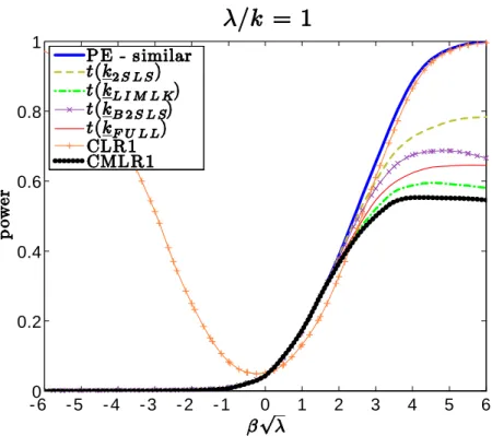
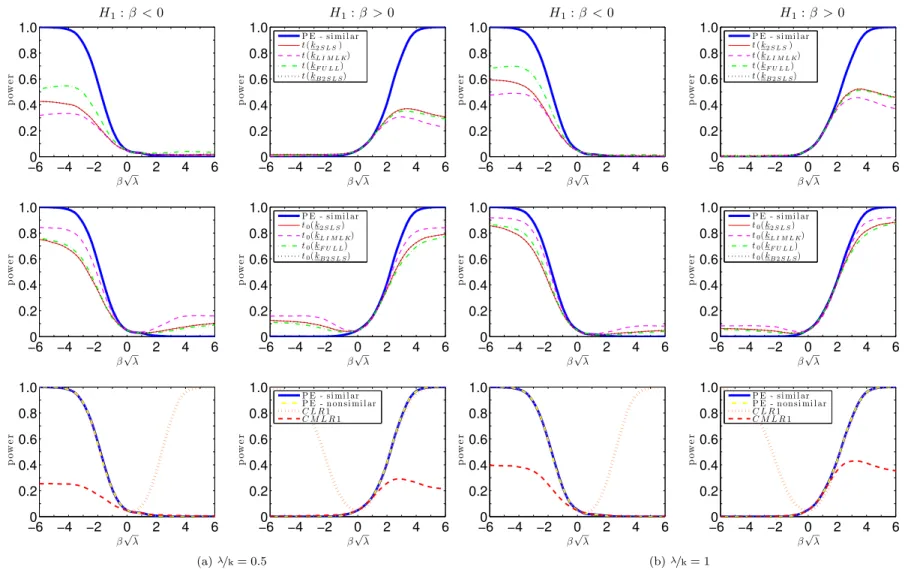
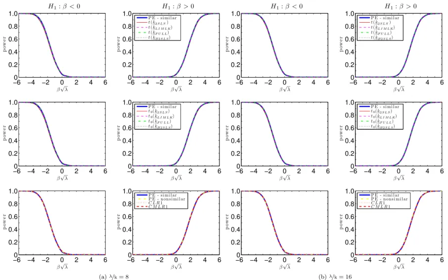
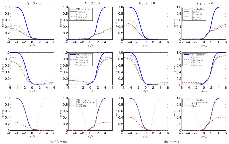
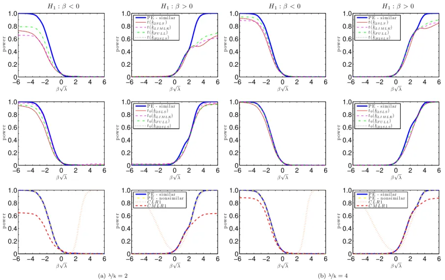
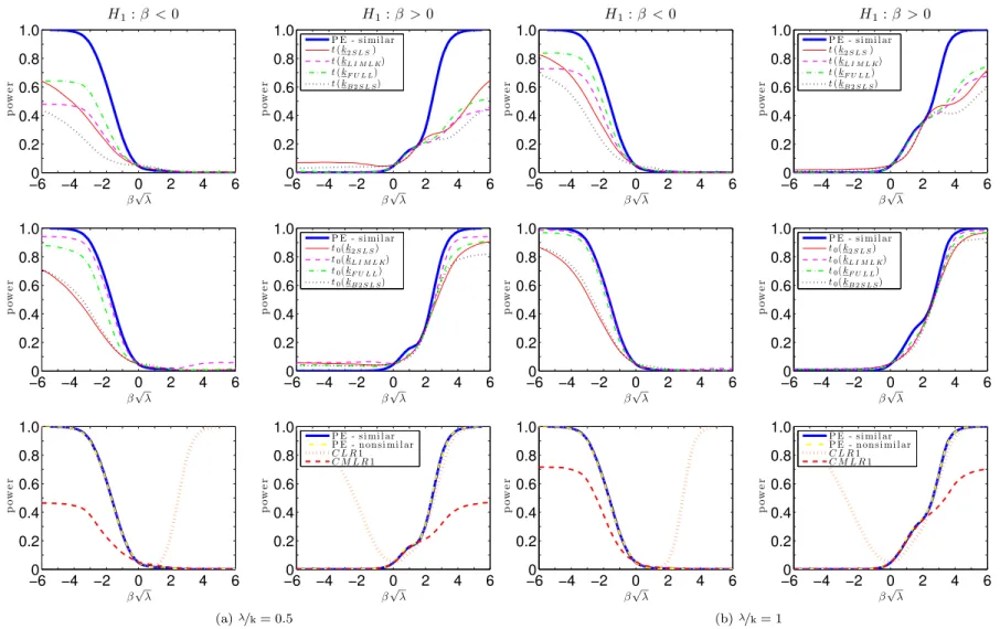
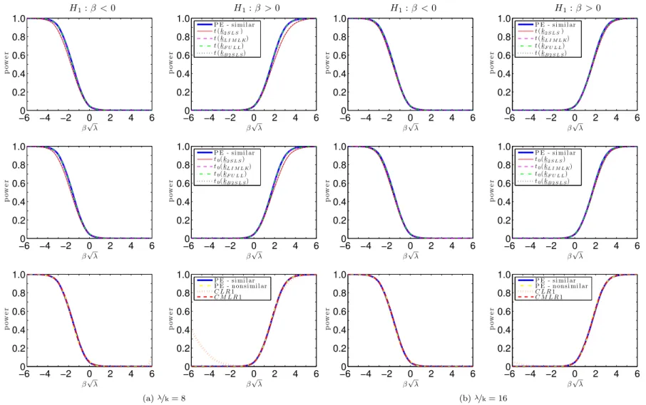
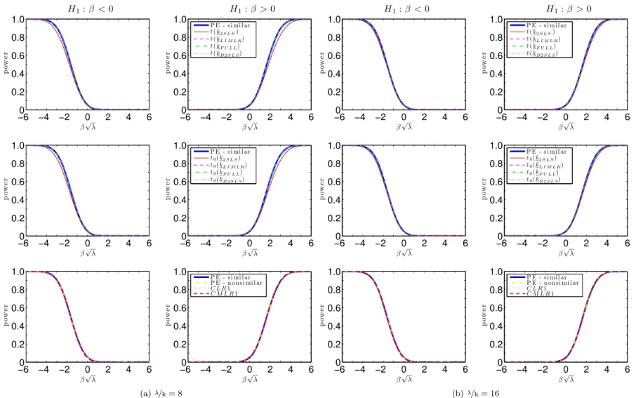
Figures7.1 and 7.2 plots the power curves for the conditional t-tests as well as both CLR1 and CMLR1 tests. Conditional critical values for all test statistics are computed based on 100,000 Monte Carlo simulations for each observed value QT =qT. In the absence of a UMPI

test, we consider tests whose power functions may be near the one-sided power envelope for invariant similar tests based on Corollary2. In the supplement, we provide numerical evidence that the power upper bounds for similar and non-similar tests are alike.

The CLR1 test has rejection probabilities close to the power upper bound for alternatives > ₀. However, this test has null rejection probabilities close to one for small enough values of < ₀. This bad behavior is in accordance with Theorem3which shows that the CLR1 test is an empirical version of POIS tests. Hence, this test is not very useful for applied researchers. Perhaps surprisingly, all four conditional t-tests perform at least as well as the CMLR1 test which has correct size for H0 : 0. When instruments are very weak ( =k = 1), the

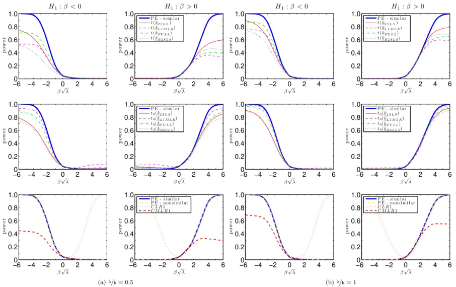
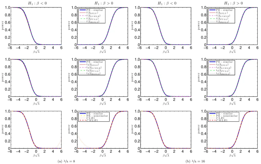
conditional t-test based on the 2SLS seems to dominate the remaining tests. As increases, the power of the conditional t-tests approaches the conservative power envelope. This result is in accordance with chapter6, which shows that the conditional t-tests are asymptotically e¢cient under strong-instrument asymptotics (SI-AE). Numerically, the conditional t-tests perform near the power envelope even when =kis as small as2. The supplement provides further evidence for

11_{There is no loss of generality in taking}

0 = 0because the structural equation y1 =y2 +X 1+u and

hypothesisH0 : = 0 can be transformed intoye1=y2e+X 1+uand H0:e= 0;whereye1=y1 y2 0 and

28

- 60 - 5 - 4 - 3 - 2 - 1 0 1 2 3 4 5 6 0.2

0.4 0.6 0.8 1

Figure 7.1: Power curves for the one-sided conditional tests when nk= 1

- 60 - 5 - 4 - 3 - 2 - 1 0 1 2 3 4 5 6 0.2

0.4 0.6 0.8 1

29

Chapter 8

Two-Sided Tests

In the present chapter we will revise the AMS07’s …nding for the conditional t-tests in the two-sided hypothesis:

H0 : = 0 againstH1: 6= 0: (8.1)

In chapter 7 and in the supplements we presented numerical results showing a good per-formance for the one-sided conditional t-tests, this is striking given the bad perper-formance of the two-sided conditional t-tests documented by AMS07. The goal of this chapter is to solve this apparent counterintuitive result between one-sided and two-sided conditional t-tests.

It turns out that AMS07’s …nding strongly relies on the asymmetry of the null conditional distribution of the t-statistics considered. Figures8.1 and 8.2plots the standard normal distri-bution with the null conditional distridistri-butions for thet(k)statistics based on the 2SLS, LIMLK,

Fuller and B2SLS to constrast this asymmetry. When the instruments are strong, ilustrated in Figure 8.1, the null conditional distribution of the t-statistics are symmetric around zero and we can use a symmetric critical value function in the two-sided test without loss of power.

- 3 - 2 - 1 0 1 2 3

0 0.1 0.2 0.3 0.4 0.5 0.6

Figure 8.1: Null conditional distribution oft(k) whenln(qT=k) = 4.

31

- 3 - 2 - 1 0 1 2 3

0 0.1 0.2 0.3 0.4 0.5 0.6

Figure 8.2: Null conditional distribution oft(k) whenln(qT=k) = 1.

To overcome this asymmetry we propose two methods: the …rst method augment the condi-tional argument of (19, Moreira (2003)) in a manner to obtain two critical value functions; the second method use other t-statistics, which are approximately symmetric, in the construction of the t-tests.

Hereinafter, it is convenient to work with the statistics

Q(k 1) =S0MTS,LM1 =QST=Q1T=2, and QT; (8.2)

which are a one-to-one transformation ofQ.

For testingH0 : = 0 againstH1: 6= 0, Theorem 1 of AMS06b proves that an unbiased

test must satisfy

E ₀ Q_{(k 1)}; LM1; qT = and (8.3)

E ₀ Q(k 1); LM1; qT LM1 = 0 (8.4)

for almost all values ofqT. By Corollary 1 of AMS06b, the CLR test satis…es both boundary

conditions. Other conditional tests – such as tests based on t(k)2– do not necessarily satisfy

(8.4). This places considerable limits on the applicability of conditional method of generating unbiased tests.

For this consider the two-sided unbiased tests based on one-sided statistics t(k) in (3.8)

which reject the null when

t(k)< _{t(k);1 x} (qT) ort(k)> t(k); x (qT); (8.5)

where t(k);x (qT)is the1 x quantile of the conditional distribution andx 2[0; ]is chosen

to approximately satisfy (8.3) and (8.4). Inverting the approximately unbiased t-tests in (8.5) allows us to construct con…dence regions around a chosen estimator (we do not obtain equal-tailed two-sided intervals, otherwise the test would be biased). In particular, we can construct con…dence regions based on the 2SLS estimator, which is commonly used in applied research.

Implicit the conditional t-test used in AMS07 consider a symmetric null distribution oft(k)

conditional onqT. Given that andx = =2 we have

32

Consequently, the test that reject the null when (8.5) is equivalent as the test that rejects the null whent(k)2 > t(k); =2(qT) 2. That is, we would have obtained the conditional test based

ont(k)2 where the critical value function is _t(k)2

; (qT) = t(k); =2(qT) 2.

The second method considered use t-tests based on modi…cations of the t-statistic that are approximately symmetric. Figures 8.3 and 8.4 plots the null conditional distribution for the modi…ed versions of t-statistics:

t0(k) =

(k) ₀

0 [y20 PZy2 n(k 1)!22] 1=2

; (8.7)

which we use 2

0= (1; 0)0 (1; 0) as the estimator of the variance of structural error.

The conditional distributions for thet0(k)statistics based on the 2SLS and Fuller estimators

are also asymmetric around zero whenqT is small. However, the t0(k) statistic for the LIMLK

estimator is nearly symmetric around zero for any value ofqT. Hence, the conditional test based

on t0(kLIM LK)2 is nearly unbiased and should not su¤er the bad power properties found by

AMS07 for thet(k)2 statistics.

- 3 - 2 - 1 0 1 2 3

0 0.1 0.2 0.3 0.4 0.5 0.6

Figure 8.3: Null conditional distribution of t0(k) when ln(qT=k) = 4.

In the supplement, we provide numerical results showing that the conditional t-test based on thet0(kLIM LK)2 statistic and some of the unbiased t-tests can perform as well as the CLR

33

- 3 - 2 - 1 0 1 2 3

0 0.1 0.2 0.3 0.4 0.5 0.6

Part I

35

Derivation of the t-Statistics

The k-class estimator for the model (2.6) is given by:

(k) = [y

?0

2 (I kMZ)y1?]

[y?0

2 (I kMZ)y2?]

; (8.8)

whereY?= [y₁?; y?₂] =MXY and the fourk-class used are:

2SLS: k= 1;

LIMLK: k=kLIM LK =Smallest root ofj(Y0PZY =n+ ) j= 0

B2SLS: k=n=(n k+ 2);

Fuller: k=kLIM LK 1=(n k p):

(8.9)

Consequently the t-statistics follows:

t(k) = (k) 0 u(k)[y?

0

2 (I kMZ)y2?] 1=2

, where

2

u(k) = b(k)0 b(k) andb(k) = (1; (k))0: (8.10)

Since we known we can simplify some expressions:

[y?₂0(I kMZ)yl?] = [y?

0

2 PZyl? (k 1)y?

0

2 MZy?l ]

= [y2PZyl n(k 1)(n k p)=n e02Y0MXMZY el=(n k p)] = [y2PZyl n(k 1)(n k p)=n wb2l]

= [y2PZyl n(k 1)w2l] +op(1); (8.11)

forl= 1;2and where the last equality follows from the fact that ^ _{is a consistent estimator for}

, (n k p)=n= 1 +o(1)and n(k 1) =Op(1) (this last result is derived from (8.9), (8.15)

and (3.3)).

So the t-statistic can be simpli…ed too:

t(k) = (k) 0

u(k)[y02PZy2 n(k 1)!22] 1=2

, where

(k) = [y

0

2PZy1 n(k 1)!21]

[y0

2PZy2 n(k 1)!22]

;

2

u(k) = b(k)0 b(k)and b(k) = (1; (k))0: (8.12)

Now we will derive the t-statistic as a function ofQ. First we will prove that thek’s for the k-class estimators are function ofQ, in particular we just need to prove that thek_{LIM LK} is ( the others follows trivially). By de…nitionk_{LIM LK}is the smallest root of_j(Y0PZY =n+ ) j= 0,

given that and considering the orthogonal matrix:

J = "

1=2_b

0

p

b0

0 b0

:

1=2_a

0

p

a0

0 1a0

#

; (8.13)

we can …nd the roots:

j(Y0PZY =n+ ) j= 0

, jJ0 1=2Y0PZY 1=2J n( 1)I2j= 0 becausejJj= 1

36

Consequently the smallest root gives us the k_{LIM LK}:

k_{LIM LK} = 1 + 1

2n(QS+QT

q

(QT QS)2+ 4Q2_ST)

= 1 + 1

n(QS LR): (8.15)

Second, de…ne:

(Z0Z) 12Z0y

l = [S:T]J0 1 2e

l

= flS+glT , (8.16)

wherefl=b00 el= p

b0₀ b0 andgl =a00el= p

a0₀ 1_a

0 forl= 1;2. So we can write the t-statistics

as:

t(k) = (k) 0

u(k)[f₂2QS+g22QT + 2f2g2QST n(k 1)w22] 1=2

, where

(k) = f1f2QS+g1g2QT + (g1f2+f1g2)QST n(k 1)w21

f2

2QS+g22QT + 2f2g2QST n(k 1)w22

,

2

u(k) = b(k)0 b(k) and b(k) = (1; (k))0: (8.17)

When we do not known the tests statistics need to consider the estimation of . The t-statistics and thek-class estimator of follows:

b

t(bk) = b(bk) 0 bu(bk)[y?0

2 (I bkMZ)y2?] 1=2

,

b(bk) = y

?0

2 (I bkMZ)y1?

y?0

2 (I bkMZ)y2?

, where _b2

u(bk) =

[y₁? y?₂b(bk)]0[y₁? y₂?b(bk)]

n 1 ; (8.18)

wherek’s are given by: 2SLS: bk= 1

LIML: bk=bkLIM L=smallest root of Y?0Y? Y?0MZY? = 0

B2SLS: bk=n=(n k+ 2)

Fuller: bk=bkLIM L 1=(n k p):

(8.19)

Using the same arguments as before, thekfor LIML estimator can be written as function of

b

Qn:

b

kLIM L = 1 + 1

n k p(QbS;n dLRn); (8.20)

asb(bk):

b(bk) = y2PZy1 (bk 1)(n k p) wb21

y2PZy2 (kb 1)(n k p) wb22

= fb1fb2QbS;n+gb1gb2QbT;n+ (gb1fb2+fb1bg2)QbST;n (bk 1)(n k p) wb21 b

f2

2QbS;n+bg22QbT;n+ 2fb2bg2QbST;n (bk 1)(n k p)wb22

; (8.21)

wherefbl=b00bnel= q

b0

0bb0 and bgl=a00el=

q

a0

0bn1a0 forl= 1;2, and b2u(bk):

b2u(bk) =

[y?₁ y?₂ b(bk)]0[y₁? y₂?b(bk)]

n 1

= bb(bk)0(Y

0_P

ZY

n 1 +

Y0MXMZY

n 1 )bb(bk)

= bb(bk)0(b

1=2_JbQJb 0_b1=2

n 1 +b

(n k p)

37

wherebb(bk) = (1; b(bk)). Finally, t-statistic is a function of Qbn :

b

t(bk) = b(bk) 0 bu(bk)[fb2

2QbS;n+bg22QbT;n+ 2fb2bg2QbST;n (bk 1)(n k p)wb22] 1=2

: (8.23)

Derivation of the One-sided Likelihood Ratio Statistics

Ignoring an additive constant, the log-likelihood function for known with all parameters concentrated out except is

lc(Y; ; ) =

n

2ln det( ) 1 2 tr(

1_Y0_M

XY) +R( ) : (8.24)

Hence, we have

LR1 = 2 "

sup 0

lc(Y; ; ) lc(Y; 0; )

#

=R( ₀) inf 0

R( ): (8.25)

We now determineinf ₀R( ):By de…nition, (k_{LIM LK})maximizeslc(Y; ; )over 2R:

Equivalently, (k_{LIM LK}) minimizes R( )over ₂R:If (k_{LIM LK}) ₀;theninf ₀R( ) = inf 2RR( ) =R( (kLIM LK))andLR1 =R( 0) inf 2RR( ) =LR:If (kLIM LK)< 0;then

inf ₀R( ) equals either R( ₀) or R(₁) because R( )is the ratio of two quadratic forms in with positive de…nite weight matrices. Hence, the second equality in (3.11) holds. A similar reasoning yields (3.13).

To see thatLR1 andM LR1 are function ofQwe just need to prove thatR( )is a function ofQ, for this note that

R( ) = b

1=2_JQJ0 1=2_b

b0 _b : (8.26)

Furthermore, we have that:

R( ₀) = QS and

R(₁) = y

0

2PZy2

w22

= f

2

2QS+g22QT + 2f2g2QST

w22

: (8.27)

Proof of Theorem 1: The power function is given by

K( ; ; ) = Z

R+ _{R R}+

(q1; qT)fQ1;QT(q1; qT; ; )dq1dqT: (8.28)

We want to …nd a test that maximizes power at ( ; ) among all level invariant similar tests. By Theorem 2 of AMS06a, invariant similar tests must be similar conditional onQT =qT

for almost all qT: In addition, the unconditional power equals the expected conditional power

given QT:Hence, it is su¢cient to determine the test that maximizes conditional power given

QT = qT among invariant tests that are similar conditional on QT = qT; for each qT. By the

Neyman-Pearson Lemma, the test of signi…cance level that maximizes conditional power given QT = qT is of the likelihood ratio (LR) form and rejects H0 when the LR is su¢ciently large

(part a) or small (part b). In particular, the conditional LR test statistic is

LR (qS; qST; qT) =

f_Q1jQT(q1jqT; ; )

f_Q1jQT(q1jqT; 0)

= fQ1;QT(q; ; )

fQT(qT; ; )fQ1jQT(q1jqT; 0)

: (8.29)

From the densityfQ1;QT(q1; qT; ; )given in (3.3), we can determinefQT(qT; ; )andfQ1jQT(q1jqT; 0)

to provide the explicit expression for LR (Q1; QT) that appears in (4.1); see Lemma 3 of

38

Proof of Theorem 3. First, we rewriteLR1in a form that is closer to that ofe_b. Ignoring an additive constant, the log-likelihood function (after concentrating out ) can be written as

l(Y; ; ; ) = n 2 lnj j

1 2tr

1_V0_M

XV ; whereV =Y Z a0 X : (8.30)

Maximizing (8.30) with respect to , one …nds that ( ) = (Z0Z) 1Z0Y 1a=a0 1a; where a ( ;1)0. The concentrated log-likelihood function,lc(Y; ; ), de…ned asl(Y; ; ( ); ), is

given by

lc(Y; ; ) =

n

2 lnj j 1 2 tr(

1_Y0_M

ZY)

a0 1Y0PZY 1a

a0 1_a : (8.31)

We can simpli…es the last term in (8.31):

(Q; ; ) = a

0 1_Y0_P

ZY 1a

a0 1_a (8.32)

= a

0 1=2_J(J0 1=2_Y0_P

ZY 1=2J)J0 1=2a

a0 1=2_JJ0 1=2_a

= ea

0_Qea

e

a0_ea ; whereea=J

1=2_a:

When evaluated atb, the maximum likelihood estimator of underH1 : > 0, (8.31) becomes

lc(Y;b; ) =

n

2lnj j 1 2

h

tr( 1Y0Y) (Q;b; )i: (8.33)

BecauseLR1is de…ned as 2[lc(Y;b; ) lc(Y; 0; )], it follows that

LR1 = 2[lc(Y;b; ) lc(Y; 0; )] = (Q;b; ) QT. (8.34)

Since the termQT can be ignored for conditional testing, the CLR1 test is equivalent to rejecting

H0 when (Q;b; )> ; (QT). Because the vectorba= (b;1)0 maximizes (8.31),

(Q;b; ) =x0_bQx_b; where x_b = (c_b=_jjh_bjj; d_b=_jjh_bjj)0: (8.35)

This proves the equivalence between the CLR1 test and the empirical POIS test based on

e_b =x0_bQx_b.

Proof of Theorem 4.

For parts (a)(i) and (b)(i) note that bt(bk)n in (8.23) is a (almost everywhere) continuous

function of Qbn and t(k1); (:) is a continuous function of QbT;n. The result follows from the continuous mapping theorem.

By the same arguments we have the results of parts (a)(ii)-(iv) and (b)(ii)-(iv).

The tests are asymptotically similar at level by de…nition of the critical value functions.

Proof of Lemma5. For part (a), we need to analyze t-statistics based on the 2SLS, B2SLS, LIMLK and Fuller estimators. The null distribution of the t-statistics conditional onQT =qT

depends on the null distribution ofQS and S2.

After some calculation, the t-statistic can be written as:

t(k) = [f2QS+g2QST] [f2

2QS+g22QT + 2f2g2QST n(k 1)w22]1=2

0

u(k)

n(k 1)(w12 w22 0)

u(k)[f22QS+g22QT + 2f2g2QST n(k 1)w22]1=2

39

For the 2SLS estimator the second term is zero and the null conditional distribution on QT =qT of the t-statistic is:

t(1) =

[f2 g2

QS

q1_T=2 +S2Q

1=2

S ]

[1 + f22 g2 2

QS

qT + 2

f2 g2S2

Q1_S=2 q_T1=2]

1=2

0

u(1)

! dS2Q1_S=2 =LM1 asqT !p1 (8.37)

because (1)_{!p 0} and u(1)!p(b00 b0)1=2= 0 asqT !p 1

The same limiting result holds for the t-statistic based on the B2SLS estimator.

Now lets analyse the t-statistic based on the LIMLK estimator. First, by expression (A.12) of AMS06a, the null conditional distribution of the LR statistics converges to chi-square-one as qT !p1 :

LR = 1

2 QS qT + (qT QS) 1 +

2qT (qT QS)2

Q_SS22 +op(1)

= Q_SS22+op(1); (8.38)

and then n(k_{LIM LK} 1)=q_T1=2 _!p 0 as qT !p 1. Second, the null conditional distribution of

the LIMLK estimator of converges in probability to 0 asqT !p 1 :

(k_{LIM LK}) =

f1f2Q_qTS +g1g2+ (g1f2+f1g2)S2Q

1=2

S

q1_T=2

n(k_{LIM LK} 1)w21 qT

f2 2QS

qT +g

2

2+ 2f2g2

S2Q 1=2

S

q1_T=2

n(k_{LIM LK} 1)w22 qT

! p

g1

g2

= ₀; (8.39)

consequently u(kLIM LK) !p 0 when qT !p 1. Finally the null conditional distribution of

t(k_{LIM LK}) converges in distribution to standard normal distribution:

t(k_{LIM LK}) =

[f2QS

g2q 1=2

T

+_S2Q1S=2]

[1 +f22 g2 2

QS

qT + 2

f2 g2S2

Q1_S=2 q1_T=2

n(kLIM LK 1)

qT w22]

1=2

0

u(kLIM LK)

n(k_{LIM LK} 1)

g2q 1=2

T

(w12 w22 0)

u(kLIM LK)[1 + f2

2 g2 2

QS

qT + 2

f2 g2S2

Q1_S=2 q1_T=2

n(k_{LIM LK} 1)

qT w22]

1=2

! d LM1asqT !p1: (8.40)

We can obtain the same result for the t-statistic based on the Fuller estimator.

For part (b), note …rst that the null conditional distribution of maxfR( ₀) R(₁);0_ggoes to zero in probability asqT !p 1:

max (

QS(1

f₂2 w22

) g2qT1=2(

g2q1_T=2+ 2f2S2Q1_S=2

w22

);0 )

!p 0; (8.41)

and so we can apply the continuous mapping theorem to obtain:

LR11=2 = LR1=2 1(t(kLIM LK)>0) +op(1)

= _S2Q1_S=2 1(S2Q1_S=2 >0) +op(1)

40

The critical value formax_fS2Q1_S=2;0g at level (with0< <1=2) is z because

P max_fS2Q1S=2;0g z =P S2Q1S=2 z = : (8.43)

Part (c) also follows from (8.41), (8.42) and (8.43).

Proof of Theorem 6. To prove part (a) note that thek-class estimator are consistent:

(k) = f1f2 QS;n

n +g1g2 QT;n

n + (g1f2+f1g2) QST;n

n (k 1)w21

f2 2

QS;n

n +g22

QT;n

n + 2f2g2 QST;n

n (k 1)w22

! p g1

g2

= ₀;

because(k 1) =Op(n 1)for each k-class considered. Consequently, u(k)!p 0 and

t(k)n =

[f2Q_n1S;n=2 +g2 QST;n

n1=2 ] [f₂2QS;n

n +g22

QT;n

n + 2f2g2 QST;n

n (k 1)w22]1=2

0

u(k)

n1=2(k 1)(w12 w22 0)

u(k)[f22

QS;n

n +g22

QT;n

n + 2f2g2 QST;n

n (k 1)w22]1=2

! d 0TSB1=jj Tjj: (8.44)

Its easy to see that thebt bk

nstatistics are asymptotically equivalent to the correspondingt(k)n

statistics.

Part (b) trivially follows from (6.1).

For part (c), recall that theLR1n statistic is

LR1n=LRn 1( (kLIM LK)> 0) + maxfR( 0) R(1);0g 1( (kLIM LK)< 0): (8.45)

Under local alternatives,max_fR( ₀) R(₁);0_{g !}p 0 because

R( ₀) = QS;n=Op(1) and

R(₁) = (f₂2QS;n+g22QT;n+ 2f2g2QST;n)=w22!p1: (8.46)

Therefore,

LR11_n=2 = LR_n1=2 1(t(kLIM LK)>0) +op(1) (8.47) ! d ( 0TSB1)=jj Tjj 1[ 0TSB1=jj Tjj>0];

where the third equality follows from the continuous mapping theorem and the joint convergence ofLRandt(kLIM LK)to( 0_TSB1)2=jj Tjj2and 0_TSB1=jj Tjj, respectively; see AMS06a,

The-orem 6(c), regarding the convergence in distribution of LR to( 0_TSB1)2=jj Tjj2. By (6.1) we

have the same asymptotic result forLR\1n.

Part (d) also follows from (8.47) because max_fR( ₀) R(₁);0_g converges in probability

to zero.

Proof of Theorem7. For part (a), following the proof of Theorem 7 of AMS06a, we know that the one-sided LM statistic for known is LM1n = QST;n=Q1_T;n=2, which is asymptotically

e¢cient by standard results.

By Lemma5, the critical values of conditional tests based onLR1n,M LR1n, and t-statistics

converge to a standard normal 1 quantile (provided ₂ [0;1=2) for the likelihood ratio

41

The LR11n=2 and M LR1n1=2 statistics are not asymptotically equivalent to LM1n: However,

the asymptotic power of the one-sided tests based on LR11n=2, M LR11n=2, and LM1n are the

same:

P max_f( 0_TSB1)=jj Tjj;0g z = P(maxf&1+ 1=2B b00 b0 1=2;0g z )

= P(&1+ 1=2B b00 b0 1=2 z )

= P 0_TSB1=jj Tjj z ; (8.48)

where&1 N(0;1),B >0, andz is a positive critical value.

By Theorem 6, the asymptotic behavior of the tests above are the same when b_n replaces . Hence, these tests are asymptotically e¢cient when is estimated.

Proof of Lemma 8. Part (i) of the Lemma is established as follows:

Sn=n1=2 = (n 1Z0Z) 1=2n 1Z0Y b0 (b00 b0) 1=2

!p D1_Z=2 a0b0 (b00 b0) 1=2=DZ1=2 c : (8.49)

Similarly,

Tn=n1=2 = (n 1Z0Z) 1=2n 1Z0Y 1a0 (a00 1a0) 1=2

!p D1_Z=2 a0 1a0 (a00 1a0) 1=2 =DZ1=2 d : (8.50)

Part (ii) of the Lemma follows from Lemma 1 of AMS06b and part (i).

Next, we prove part (iii) of the Lemma. If = _AR;thena0 1a0 = 0and using Assumption

4, we have

Tn = (n 1Z0Z) 1=2n 1=2Z0V 1a0 (a00 1a0) 1=2 (8.51)

!d&k N(0; Ik): (8.52)

Part (iii) now follows from Lemma 1 of AMS06b.

Proof of Theorem 9: For part (a), we use Lemma 8 in (3.9) to note that (k 1) =op(1)

and consequently thek-class estimators are consistent:

(k) = f1f2 QS;n

n +g1g2 QT;n

n + (g1f2+f1g2) QST;n

n (k 1)w21

f2 2

QS;n

n +g22

QT;n

n + 2f2g2 QST;n

n (k 1)w22

! p

f1c +g1d

f2c +g2d

= ; (8.53)

if 6= _AR or = _AR, therefore u(k)!p (b0 b)1=2 = u.

Now we can show the asymptotic distribution oft(k)n=n1=2. For either 6= ARor = AR:

t(k)n p

n =

[f2QS;n_n +g2QST;n_n ]

[f₂2QS;n

n +g22

QT;n

n + 2f2g2 QST;n

n (k 1)w22]1=2

0

u(k)

(k 1)(w12 w22 0)

u(k)[fQS;n_n +g22

QT;n

n + 2f2g2 QST;n

n (k 1)w22]1=2

! p c 1_{F A}=2 0 u

: (8.54)

By the same arguments,bt(bk)n=n1=2 converges in probability toc 1_{F A}=2 0= u.

42

For parts (c) and (d), we write the LR1n statistic as in (3.11). To study the behavior of

LR1n under …xed alternatives, we use the following:

R(₁)

n = (f

2 2

QS;n

n +g

2 2

QT;n

n + 2f2g2 QST;n

n )w

1

22 !p F Aw221,

R( ₀)

n =

QS;n

n !p c

2

F A, and

LRn

n =

1 2(

QS;n

n

QT;n

n +

r (QT;n

n

QS;n

n )2+ 4 QST;n

n !p c

2

F A: (8.55)

which holds if: = _AR or ₆= _AR.

If > ₀;1( (k_{LIM LK}) ₀)_!p1 by continuous mapping theorem and so

LR1n

n !p c

2

F A: (8.56)

If < ₀;1( (k_{LIM LK}) ₀)_!p0 and

LR1n

n !pmaxfc

2 _w 1

22;0g F A: (8.57)

The same is true for LR\1n=n:

For parts (e) and (f), we write the M LR1n statistic as in (3.13).

If > ₀;1( (k_{LIM LK}) ₀)_!p1 and

M LR1n

n !p c

2

F A maxfc2 F A w221 F A;0g+c2 F A = minfc2; w221g F A: (8.58)

If > ₀;1( (k_{LIM LK}) ₀)_!p0 and

M LR1n

n !p0: