ESCOLA DE P ´
OS-GRADUAC
¸ ˜
AO EM
ECONOMIA
Gustavo Rabello de Castro
Invariant Tests in an Instrumental Variables
Model with Unknown Data Generating Process
Rio de Janeiro 2015
Invariant Tests in an Instrumental Variables Model with
Unknown Data Generating Process
Disserta¸c˜ao para obten¸c˜ao do grau de mestre apresentada `a Escola de P´ os-Gradua¸c˜ao em Economia
´
Area de concentra¸c˜ao: Econometria
Castro, Gustavo Rabello de
Invariant tests in an instrumental variables model with unknown data generating process / Gustavo Rabello de Castro. – 2015.
58 f.
Dissertação (mestrado) - Fundação Getulio Vargas, Escola de Pós- Graduação em Economia.
Orientador: Marcelo J. Moreira. Inclui bibliografia.
1. Análise de regressão. 2. Variáveis instrumentais (Estatística). 3. Testes de hipóteses estatísticas. I. Moreira, Marcelo J. II. Fundação Getulio Vargas. Escola de Pós-Graduação em Economia. III. Título.
CDD – 519.536
In this work we focus on tests for the parameter of an endogenous variable in a weakly identified instrumental variable regression model. We propose a new unbiasedness restriction for weighted average power (WAP) tests introduced by Moreira and Moreira (16, 2013). This new boundary condition is motivated by the score efficiency under strong identification. It allows reducing computational costs of WAP tests by replacing the strongly unbiased condition. This latter restriction imposes, under the null hypothesis, the test to be uncorrelated to a given statistic with dimension given by the number of instruments. The new proposed boundary condition only imposes the test to be uncorrelated to a linear combination of the statistic. WAP tests under both restrictions to perform similarly numerically. We apply the different tests discussed to an empirical example. Using data from Yogo (22, 2004), we assess the effect of weak instruments on the estimation of the elasticity of inter-temporal substitution of a CCAPM model.
Keywords: Instrumental variable regression, invariant tests, optimal tests, similar tests, unbiased tests, weighted average power tests, weak instruments.
Este trabalho trata de testes para o parˆametro de uma vari´avel end´ogena em modelos de regress˜ao com vari´aveis instrumentais fracas. Propomos uma nova restri¸c˜ao para o vi´es dos testesweighted average power (WAP), desenvolvidos em Moreira e Moreira (16, 2013). A motiva¸c˜ao para essa nova restri¸c˜ao se baseia na eficiˆencia do teste score sob a hip´otese de identifica¸c˜ao forte. Essa hip´otese permite reduzir o custo computacional dos testes WAP, substituindo a restri¸c˜ao de strongly unbiased. Esta ´ultima demanda que, sob a hip´otese nula, o teste seja ortogonal a uma dada estat´ıstica com sua dimen¸c˜ao dada pelo n´umero de instrumentos. A restri¸c˜ao aqui proposta exige somente que o teste seja n˜ao correlacionado com uma combina¸c˜ao linear dessa estat´ıstica. Nas simula¸c˜oes, ambos os testes apresentam um desempenho numericamente similar. Aplicamos ainda os testes discutidos neste trabalho na estima¸c˜ao da elasticidade de substitui¸c˜ao intertemporal de um modelo CCAPM.
Palavras-chave: Regress˜ao com vari´aveis instrumentais, testes invariantes, testes ´otimos,
1 Design 3 non-kronecker with ρ= 0.2 and α= 0.9 . . . 34 2 Design 3 non-kronecker with ρ= 0.95 and α= 0.9 . . . 35 3 Simulations for Real Aggregate Stock Return as the Endogenous Variable 37 4 Simulations using Yogo data . . . 38 5 HACIV Power Comparison (Non-Kronecker Covariance): k= 2, ρ= 0.2 . 45 6 HACIV Power Comparison (Non-Kronecker Covariance): k= 2, ρ= 0.5 . 46 7 HACIV Power Comparison (Non-Kronecker Covariance): k= 2, ρ= 0.95 . 47 8 HACIV Power Comparison (Non-Kronecker Covariance): k= 5, ρ= 0.2 . 48 9 HACIV Power Comparison (Non-Kronecker Covariance): k= 5, ρ= 0.5 . 49 10 HACIV Power Comparison (Non-Kronecker Covariance): k= 5, ρ= 0.95 . 50 11 HACIV Power Comparison (Non-Kronecker Covariance): k= 10, ρ= 0.2 . 51 12 HACIV Power Comparison (Non-Kronecker Covariance): k= 10, ρ= 0.5 . 52 13 HACIV Power Comparison (Non-Kronecker Covariance): k= 10, ρ= 0.95 53 14 HACIV Power Comparison (Non-Kronecker Covariance): k= 20, ρ= 0.2 . 54 15 HACIV Power Comparison (Non-Kronecker Covariance): k= 20, ρ= 0.5 . 55 16 HACIV Power Comparison (Non-Kronecker Covariance): k= 20, ρ= 0.95 56 17 HACIV Power Comparison (Non-Kronecker Covariance): k= 50, ρ= 0.2 . 57 18 HACIV Power Comparison (Non-Kronecker Covariance): k= 50, ρ= 0.5 . 58 19 HACIV Power Comparison (Non-Kronecker Covariance): k= 50, ρ= 0.95 59
1 Introduction 9
2 Linear IV Regression Model 10
2.1 Linear IV Model Under Homoskedastic Errors . . . 10 2.2 Linear IV Regression Model Under Heteroskedastic and Autocorrelated
Errors (HAC-IV) . . . 11 2.3 The Linear IV Model in a GMM Context . . . 12
3 Invariant Similar Tests Under Homoskedastic Errors 14
4 AR, LM and CLR Generalizations to HAC Errors 15
5 Power Envelope 17
6 Plug-In Minimax Regret Test 19
7 WAP Tests 22
7.1 WAP-LU Tests . . . 23 7.2 WAP-SU Tests . . . 24 7.2.1 Algorithm . . . 24
8 WAP-Score Test 26
9 Invariance Under HAC Errors 29
10 Simulation Designs 33
1
Introduction
In instrumental variable regression, instruments are said to be weak when they are poorly correlated to the endogenous regressors. It is well known that, under weak iden-tification, standard asymptotic theory can not be employed to develop reliable inference methods. In particular, the usual tests and confidence regions do not have correct size. In this work, we revisit the literature for identification-robust hypothesis tests in instrumental variable regression. These tests control size regardless of identification strength, limiting the probability of rejecting the true hypothesis in weakly identified models. Our first step is to introduce the following standard weak instrument tests: Lagrangian Multiplier (LM) test; Anderson-Rubin (1, AR, 1947) test; and Moreira (13, 2003) Conditional Likelihood Ratio (CLR) test. Thereafter, we introduce the novel Minimax Plug-In Conditional Linear Combination (PI-CLC) test introduced by Andrews (5, 2014). Finally, we present Moreira and Moreira (16, 2013) Weighted Average Power (WAP) tests.
We propose a new unbiasedness boundary condition for WAP tests introduced by Moreira and Moreira (16, 2013). This new boundary condition is motivated by the score efficiency under strong identification. It allows reducing computational costs of WAP tests by replacing the strongly unbiased condition. This latter boundary condition imposes, under the null hypothesis, the test to be uncorrelated to a given statistic with dimension given by the number of instruments. On the other hand, the new restriction only imposes the test to be uncorrelated to a linear combination of the statistic. WAP tests under both restrictions perform similarly numerically.
In this paper, we revise the literature for weak instruments inference with a particular emphasis on power. Indeed, the major part of this literature focus on size, and to date the results on power of identification-robust tests are quite limited. Therefore, we intend develop a new simulation designs and carry on an extensive number of simulations in pursuit of good power properties.
Finally, we apply the different tests discussed in this paper to an empirical example. Using data from Yogo (22, 2004) we assess the effect of weak instruments on the esti-mation of the elasticity of inter-temporal substitution of a Consumption Capital Asset Pricing Model-CCAPM.
2
Linear IV Regression Model
In this paper we study linear instrumental variable regression models with the objective of making inference about the coefficient of the endogenous variable when the instru-ments are possibly weak. More specifically, we want to test β in the following linear model:
y1 = y2β+u,
y2 = Zπ+v2, (1)
where y1, y2 ∈ Rn, and Z ∈ Rn×k are observable variables; u, v2 ∈ Rn are unobserved
errors ; andβ ∈R, and π ∈Rk are unknown parameters. The matrixZ is taken to be fixed (i.e., non-stochastic) and has full column rankk.
In this paper we are interested in two-sided hypothesis testing of the coefficient β :
H0 :β =β0 againstH1 :β6=β0 (2)
Furthermore, the model can be rewritten as a matricial reduced-form:
Y =Zπa′+V, (3)
whereY = [y1:y2] ,V = [v1:v2] = [u+v2β:v2] and a= (β,1)′,
2.1 Linear IV Model Under Homoskedastic Errors
[S:T], where
S = (Z′Z)−1/2Z′Y b0·(b′0Ωb0)−1/2 and
T = (Z′Z)−1/2Z′YΩ−1a0·(a′0Ω−1a0)−1/2, (4)
whereb0 = (1,−β0)′ and a0= (β0,1)′.
The distribution of the sufficient statistic [S:T] is multivariate normal,
vec[S:T]∼N(hβ⊗µπ, I2k), (5)
with first moment depending on the following quantities:
hβ = (cβ, dβ)′∈R2 and µπ = (Z′Z)1/2π∈Rk, (6)
wherecβ = (β−β0)·(b′0Ωb0)−1/2 anddβ =a′Ω−1a0·(a0′Ω−1a0)−1/2.
2.2 Linear IV Regression Model Under Heteroskedastic and
Autocor-related Errors (HAC-IV)
In this section we drop the assumption of V beeniid across rows and allow the reduced-form errors to have a more general covariance matrix. Following Moreira and Moreira (16, 2013), we defineP1 =Z(Z′Z)−1/2 and choose P = [P1, P2]∈On, the group of nxn
orthogonal matrices. Pre-multiplying the reduced form model by P’, we have
P1Y
P2Y
!
= µa′ 0
!
+ W1
W2
!
(7)
whereµ= (Z′Z)1/2π. Moreira and Moreira (16) consider only tests base on P1′Y
(Z′Z)−1/2Z′Y =µa′+W1 (8)
Assuming thatW1 ∼N(0,Σ), the sufficient statistic for the model set by equation 8 is
given by the pair
S = [(b′
0⊗Ik)Σ(b0⊗Ik)]−1/2(Z′Z)−1/2Z′Y b0
and
T = [(a′
0⊗Ik)Σ−1(a0⊗Ik)]−1/2(a0⊗Ik)Σ−1vec[(Z′Z)−1/2Z′Y]
2.3 The Linear IV Model in a GMM Context
The identifying assumption in instrument variable models is thatE[uiZi] = 0. Naturally, we can see linear IV as a special case of generalized method of moments (GMM) with moment condition given by:
fi(β) = (y1,i−y2,iβ)Zi
and identifying assumptionEβ[fi(β)] = 0, where the expectation is taken under the true
parameter valueβ.
To derive the limit problem for a GMM model under weak identification, we follow Staiger and Stock (18, 1997), modeling the first stage parameterπ as changing with the sample size: πN = √cN for a fixedc∈Rk.
Defining fN(β) = Pfi(β)/N and letting Ψ be the asymptotic variance matrix of √
NfN(β0)′,−∂β∂ fN(β0)′
Ψ = "
Ψf f Ψf β
Ψf β Ψf β
#
= lim N→∞ V ar
"
√
N fN(β0) −∂β∂ fN(β0)
!#
(9)
Re-writing the moment condition, we have that
fN(β0) =fN(β0)−fN(β) +fN(β) = N1 P(y2,iβ−y2,iβ0)Zi+fN(β)
Note that the expectation offN(β), under the true parameter,β is zero by the
identifi-cation assumption, so
EβfN(β0) = N1E[Z′y2](β−β0).
Since
Assuming that Ψ1is known, and defininggN(β) = √
NΨ−f f1/2fN(β)/N and ∆gN(β) = √
NΨ−f f1/2∂β∂ fN(β), we have
gN(β0)
∆gN(β0)
!
→ d
g
∆g
!
∼
N
Ψ−f f1/2QZc(β−β0)
Ψ−f f1/2QZc
!
, I Ψ
−1/2
f f Ψf βΨ−f f1/2
Ψ−f f1/2ΨβfΨ−f f1/2 Ψ−f f1/2ΨββΨ−f f1/2
!!
Now, following Kleibergen (2005), we define D as
D= ∆g−Ψf f−1/2Ψf βΨ−f f1/2g
and note that
g
∆g
!
∼N
Ψ−f f1/2QZc(β−β0)
d
!
, I 0
ΨD
!!
where d = Ψ−f f1/2QZc(I −(β −β0)) and ΨD = Ψf f−1/2ΨββΨ−f f1/2 −(Ψf f−1/2Ψf βΨ−f f1/2)2.
That is, D is the part of ∆g that is independent of g and is informative about the identification strength and can be seen as a transformation of the first-stage parameter estimate.2 Making a relationship with the S and T statistics from Moreira and Moreira (2013), note that
Σ = (Z′Z−1/2⊗I2)
"
Ψf f+β2Ψββ+ 2βΨf β Ψf β+βΨββ
Ψf β+βΨββ Ψf β+βΨββ
#
(Z′Z−1/2⊗I2),
where g is up to rotation equal to S and D plays the role of T3 .
1Or ˆΨ a consistent estimator of Ψ 2
See Moreira(12, 2002) for homoskedastic linear IV model
3
Invariant Similar Tests Under Homoskedastic Errors
In this section, we present some of the main hypothesis tests for the weakly identified linear IV model, under homoskedastic errors presented in section 2.1. Andrews, Moreira and Stock (3, 2006) developed a theory of optimal hypothesis testing when instruments can be weak, and used that theory to derive practical hypothesis tests that are nearly op-timal, independent of the strength of identification. For that purpose they have adopted a natural invariance condition that the decision to reject or not the null hypothesis do not change with the order in which each instrument appears, i.e., if the instruments are transformed by an orthogonal matrix. As a consequence we restrict our analysis to tests that are invariant to orthogonal transformations. That is: let φbe a [0,1]-valued statistic depending on the sufficient statistics [S : T]; and F be a k×k orthogonal matrix. The tests considered are such thatφ(F S, F T]) =φ(S, T).
By Theorem 1 of Andrews, Moreira and Stock (3, 2006), a test is invariant if and only if it can be written as a function of
Q= [S:T]′[S:T] = "
S′S S′T T′S T′T
# =
"
QS QST QST QT
#
. (11)
Usual examples of invariant test statistics are the Anderson and Rubin (1, 1949) (AR), score and Moreira (13, 2003) conditional likelihood ratio statistics:
AR = QS/k, LM = Q2ST/QT,
LR = 1
2
QS−QT +
q
(QS−QT)2+ 4Q2ST
4
AR, LM and CLR Generalizations to HAC Errors
In this section we generalize the hypothesis tests presented in section 3, allowing for more general covariance structures. Examples of two-sided HAC-IV similar tests are: the S-test (Stock and Wright (19, 2000)), which is the generalized version of the AR test for heteroskedastic errors; K-test Kleibergen’s (9, 2005) generalization of the score test; and the Conditional Quasi-Likelihood Ratio test (CQLR), Kleibergen’s (9, 2005) generalization of CLR test.
Following Stock and Wright (19, 2000), we define the heteroskedasticity robust weighting matrix
V(β) =T−1P
fi(β)fi(β)′
and the objective function
S(β, β) = [T−1/2P
fi(β)]′V(β)−1[T−1/2P
fi(β)]
by Stock and Wright theorem 2, S(β0, β0) is asymptotically distributedχ2k and thus do
not depend on the nuisance parameter. Therefore, confidence intervals forβ with correct coverage can be computed by inverting the objective function above.
Also, notice that we can writeS(β, β) as
S-test =g′g
Finally we have
φS =I{S-test> χ2k,1−α}
whereχ2k,1−α stands for the 1−α quantile of a chi-square-k distribution. Kleibergen (9, 2005) defines the statistic
K=g′PDg
where PD =D(D′D)−1D′. Using the fact that D and g are independent we can show, thatK ∼χ21. Thus,
φK =I{K > χ21,1−α}
We can also write these tests as functions of statistics S and T. S-test can be written as (Moreira and Moreira (17, 2013))
On the other hand, the score statistic is given by (Moreira and Moreira (17, 2013))
LM = S
′C
β0D−
1
β0T q
T′D−1
β0C
2
β0D
−1
β0T
It is well known that the AR test is optimal when the model is just-identified. How-ever, it has poor power properties when the model is over-identified, since the degrees of freedom is larger than the number of parameters being tested. On the other hand, the score test is optimal under strong identification but can choose random directions for some alternatives when instruments are weak.
A natural generalization of Moreira (13, 2003) CLR would be using the generalized statistics presented above. Therefore, we define the CQLR as
CQLRr= 12AR−r(D) +p(AR+r(D))2−4(AR−K)r(D)
wherer(D), in a GMM context, corresponds to a rank statistic that allows for a general covariance matrix. One of the possible rank statistics that can be used is Cragg and Donald (8, 1997) rank statistics, that under one endogenous variable simplifies to
r(D) =D′Φ−D1D
Under the null hypothesis the CQLR statistic has distribution
1 2
χ2k−r(D) +q(χ2
k+r(D))2−4χ2k−1r(D)
Thus,
φCQLRr =I{CQLRr>
χ2k−r(D) +q(χ2k+r(D))2−4χ2
k−1r(D)
5
Power Envelope
After presenting some of the weak IV robust tests, we construct a power envelope to help comparing them. There are several ways to construct a two-sided power enve-lope, depending on how we impose the two-sidedness condition. There are three main approaches mentioned in Andrews, Moreira and Strock (3, 2006). The first one consid-ers the average power for β values less than and greater than the null hypothesis. The second imposes a sign invariance condition, and the third imposes a necessary condition for unbiasedness.
There are two necessary condition considered in the literature for unbiasedness: the locally unbiased and the strongly unbiased.
From proposition 3 of Moreira and Moreira (17, 2013): A test is said to be locally unbiased (LU) if
Eβ0,µφ(S, T)S′Cβ0µ= 0,∀µ
If a test is unbiased, then it is similar and locally unbiased
The LU condition imposes that the test φ is uncorrelated to a linear combination of the pivotal statistic S, weighted by the instruments’ coefficient µ, under the null hypothesis.
A sufficient condition for the LU is the strongly unbiased condition (SU)
Eβ0,µφ(S, T)S = 0,∀µ
The LU condition states that the test is uncorrelated to the statistic S under the null hypothesis. Naturally, the LU condition holds if the SU condition holds. However, as lemma 1 of Moreira and Moreira (17, 2013) shows, there are tests which satisfy the LU condition but not the SU condition. Hence, the power envelope based on the SU condition must have power lower or equal than the power envelope based on the LU condition.
Proposition 4 of Moreira and Moreira (17, 2013), analogous to Theorem 2-(c) of Moreira (15, 2009) for the homoskedastic case, sets a test that maximizes the power for a given alternative (β, µ), given the SU constraint and similarity constrain, i.e.,
Z
φfβ0,µ =α and R
φsfβ0,µ = 0, ∀µ
(s′Cβ0µ)
2
µ′C2
6
Plug-In Minimax Regret Test
In this section we present one of the new tests available in the literature that seeks for good power properties. I. Andrews (5, 2014) introduce the class of conditional linear combination tests (CLC tests), which reject the null when a convex combination of two weak identification robust statistics is large. He shows that this class of test is equivalent to a class of conditional quasi-likelihood ratio tests, in particular, that the conditional likelihood test of Moreira (13, 2003) is a conditional linear combination test. Andrews paper proposed using a minimax conditional linear combination test and suggests a computational tractable class of tests that plug in an estimator for a nuisance parameter. It is clear that the minimax plug-in conditional linear combination test will not be a true minimax CLC test, but apparently this feasible version performs well in simulation.
Andrews (5, 2014) work relied on two innovations: first, he introduced a novel class of procedures, the class of conditional linear combination tests. Second, he proposed an optimality criterion that minimize maximum regret of the test with respect to the power envelope of this same class of tests.
In order to present Andrews’ plug-in CLC test, the first step is to introduce the class of conditional linear combination tests. These tests depend on a linear combination of the generalized Anderson-Rubin (AR) statistic, introduced by Stock and Writh (19, 2000), and the score (LM) statistic introduced by Kleibergen (9, 2005) for GMM models. In the latter, the weight assigned to each statistic depends on a conditioning statistic D, introduced by Kleibergen (9, 2005). The test based on the AR statistic has stable power and is optimal when there is only one single instrument, but is inefficient under strong identification and when there are many instruments. On the other hand, the test based on the LM statistic is efficient under strong identification but can have low power for some values of the alternative hypothesis. The statistic D plays the role of the statistic T defined by Moreira (13, 2003) being a sufficient statistic for the nuisance parameter and can be viewed as measuring identification strength. Therefore, the CLC tests use information from D to allocate the weight between the AR and LM statistics.
For a weight functiona:D→[0,1] the corresponding conditional linear combination test, φa(D), rejects the null hypothesis when the convex combination of AR and LM statistics, weighted by a(D), exceeds a conditional critical value:
We take the conditional critical value cα(a) to be the 1−α quantile of a χ21 +
aχ2k−1 distribution since, under the null hypothesis, LM2 ∼ χ21, AR ∼ χ2k−1 and are independent. This choice ensures that φa(D) will be conditionally similar, and thus similar, for any choice of a(D).
One interesting result from Andrews (5, 2014) states that the class of CQLR tests is the same as the class of CLC tests. That is, for any function r : D → R+ ∪ {∞}
we define the CQLR statistic CQLRr, as in section 4, and let qα(r(d)) be the 1−α
quantile of its respective null distribution. From Andrews (5, 2014) theorem 2, we define ˜
a(D) = qα(r(D))
qα(r(D)+r(D) such that φCQLRr ≡φ˜a. Conversely, for any a : D → [0,1] there
exist a ˜r :D→R+∪ {∞} such thatφa(D) ≡φCQLR˜r.
Any weight function a : D → [0,1] defines a CLC test φa(D). While any such test
controls size, the class of CLC test is large and we would like a systematic way to choose weight functions a yielding tests with good power. Therefore, the second innovation in Andrews (5, 2014) paper is to use minimax regret as an optimality criterion, selecting CLC tests with power curves as close as possible to the power envelope for this class. Minimax regret could be seen as an extreme taken as an optimality criterion. But as Vilela (20, 2014) shows in his work, minimax and maxmin criteria have good optimality properties. Indeed, if a uniformly most powerful test (UMP) exist and the minimax or maxmin testφ∗ is unique than φ∗ will be UMP. Moreover, the minimax or maxmin test always exists and there is no arbitrariness as in the weighted average power tests. However, for linear IV models, obtaining the CLC minimax regret test may be computa-tionally intractable. In this context, Andrews suggests a class of computacomputa-tionally simple plugs-in test that plugs in an estimate for a nuisance parameter. The use of an estimate for the nuisance parameter allows reducing the optimization problem from optimizing over the space of functions to optimizing over numbers in the [0,1] interval.
It is important to note that φP I treats the estimated value of µD as the true value, and hence does not account for any uncertainly in the estimation. Moreover, even if we new µD, φP I restricts attention to unconditional linear combination tests, which
represents a subset of possible functions a∈A.
One way to compare CLC tests and WAP-SU tests is noting that the class of CLC tests is a subset SU tests and thus that WAP-SU tests have, by construction, weighted average power at least as high as any CLC test under their respective weight functions. To see that CLC test is a SU test, we note that for a given D=d (or T=t) AR and LM are invariant to sign transformation of S. Since S ∼N(0, Ik) conditional on T=t under β =β0, we can see that for any conditional linear combination testφa(D)
Eβ0,µ[φa(D)S|T =t] =Eβ0,µ[−φa(D)S|T =t] = 0
7
WAP Tests
In this section we present the WAP tests based on weighted average density, as in Moreira and Moreira (16, 2013). In classical testing theory, if both hypothesis are simple, the Neyman-Person lemma establishes necessary and sufficient conditions for a test to be the most powerful among all tests with the null rejection probability no greater than
α. When the alternative is composite, the optimal test may or may not depend on the choice of the alternative. If it does depend on the alternative, a commonly used device is to reduce the composite alternative to a simple one by choosing a weighting function Λ1 and maximizing a weighted average density:
sup
0≤φ≤1
= Z
φh, where Z
φfβ0 ≤α
whereh= Z
fβΛ1dβfor some probability measure Λ1that weights different alternatives.
Moreira and Moreira (16, 2013) define two different invariant weighted average den-sities h(s,t) based on different weights Λ1. They calculate their weights using the 2x2
and kxk symmetric positive definite matrix Ω∗ and Φ∗ solving min||Σ−Ω⊗Φ||F, where
||X||F = (tr(X′X))(1/2)denotes the Frobenius norm of a matrix X. The first one is based on the weighted average densityh1(s, t) which is invariant to orthogonal transformations.
That is, it depends on the data only through Q (17, Proposition 1.a). The second one is based on the weighted average density h2(s, t) which is invariant to orthogonal sign
transformation. That is, it depends on the data only through QS, |QST| and QT (17,
Proposition 1.b). Moreover, tests depending on the data only through QS, |QST| and QT are locally unbiased (3, AMS, 2006). Hence WAP test based onh2(s, t) is a natural
two-sided test when the errors are homoskedastic (17).
sup
0≤φ≤1
Z
φh, where
Z
φfβ0,µ=α and Z
φ∂lnfβ,µ ∂β
β=β0
fβ0,µ
where the integrals are with respect to (s,t).
There are two boundary conditions in the maximization problem above. The first one states that the test is similar and the second imposes that the test is locally unbiased.
MM also consider a sufficient condition for local unbiasedness, the strongly unbiased (SU) condition which is computationally more tractable.
7.1 WAP-LU Tests
From MM, we know that LU condition simplifies to
Eβ0,µφ(S, T)S′Cβ0µ= 0,∀µ
The WAP-LU test solves the following
max
φ∈K
Z
φh, where
Z
φfβ0,µ=α and Z
φs′Cβ0µfβ0,µ= 0, ∀µ
MM propose solving the approximated maximization problem:
max
φ∈K
Z
φh,where Z
φfβ0,µ∈[α−ǫ, α+ǫ], ∀µ
and Z
φs′Cβ0µlfβ0,µl = 0,forl= 1, ..., n
when ǫis small and n is large.
The optimal test rejects the null when
h(s, t)
fβS0(s) −s
′C
β0
n
X
l=1
cǫlµlfβT0,µl(t)> q(t),
where the multiplierscǫl, l = 1, ..., nsatisfy the constraints from the problem above and
q(t) is the conditional 1−α quantile of
h(S, t)
fS β0(S)
−S′Cβ0
n
X
l=1
cǫlµlfβT0,µl(t)
Finding the multipliers using a nonlinear optimization algorithm when the number of discretizations n is large can be computationally difficult. Thus, Moreira and Moreira suggest implementing WAP-LU only for the true parameter µ∗, i.e., n=1 andµ1 =µ∗,
7.2 WAP-SU Tests
These tests maximize weighted average power, for weights on (β, µ) which depend on the covariance matrix Σ, over the class of similar tests satisfying a sufficient condition for local unbiasedness (SU tests).
The LU condition holds if
Eβ0,µφ(S, T)S= 0,∀µ(SU condition)
The WAP test derived from this condition solves
max
φ∈K
Z
φh, where
Z
φfβ0,µ=α and Z
φsfβ0,µ= 0, ∀µ
Since the statistic T is complete we can carry on a power maximization for each level T=t:
max
φ∈K
Z
φh, where
Z
φfβS0 =α and
Z
φsfβS0 = 0, ∀t
Therefore, the optimal test rejects the null when
h(s, t)
fβS0(s) > c(s, t),
where the function c(s, t) =c0(t) +s′c1(t) satisfies the boundary conditions.
7.2.1 Algorithm
Consider the approximate problem
max
0≤xj≤1
1
J J
X
j=1
xjh(sj, t)exp(sj′sj/2)(2π)k/2
for appropriate matrices A and vectors p and r. We then use standard linear program-ming (primal) to find x andc= (c1, ..., cn+1) to the dual problem
min
c∈Rn+1 p
′c
8
WAP-Score Test
We have seen, in the previous section, the weighted average power tests introduced by Moreira and Moreira (16, 2013). In this section we define a new boundary condition for the WAP tests to be unbiased. We know that φLM is asymptotically efficient under
strong identification and local alternatives. Observing that WAP tests bias becomes larger when instruments becomes strong, we will impose the test to be orthogonal to score statistic and so asymptotically equivalent to score under local alternatives. That is equivalent to state that the probability of the two tests yielding the same decision tends to one, both under a sequence of alternativesβ0+B/n.5.
Indeed, under some mild conditions Wald (21, 1943) established that LM test have large sample optimality properties. Such optimality properties include maximizing av-erage asymptotic power over certain ellipses in the parameter space and uniformly max-imizing power among asymptotically unbiased tests.
For illustration let’s consider the case of searching for a uniformly most powerful unbiased test in a Multiparameter exponential family. Following Lehmann and Romano (11, 2005), letθ be a real parameter and X a random vector with probability density
dPθ,ϑX (x) =C(θ, ϑ)exp θU(X) +
k
X
i=1
ϑiTi(x)
!
dµ(x)
and letϑ(ϑ1, ..., ϑk) andT = (T1, ..., Tk).
We can focus on the sufficient statistics (U,T) which joint distribution
dPθ,ϑU,T(u, t) =C(θ, ϑ)exp θU +
k
X
i=1
ϑiti
!
Consider the test φforH0:θ=θ0 againstH1:θ6=θ0 satisfying φ=
1 if u < c1(t) or u > c2(t)
γi(t) if u=ci(t) 0 if otherwise
withci’s and γi’s determined by
Eθ0[φ(U, T)|t] =α (restriction 1) Eθ0[U φ(U, T)|t] =αEθ0[U|t] (restriction 2)
By theorem 4.4.1 of Lehmann and Romano (11, 2005), the critical function defined byφconstitutes a UMP unbiased level-α test for testingH0:θ=θ0 against H1:θ6=θ0
when the joint distribution of U and T is given by equation 12.
Inspired by restriction 2 we can impose a new boundary condition for unbiasedness
Eβ0,µφ(S, T)S′Cβ0D−
1
β0T = 0,∀µ Indeed, note that
Eβ0,µ[φ(S, T)S′Cβ0D−
1
β0T] =αE
T
β0,µEβ0[S
′C
β0D−
1
β0 t|T =t] = 0 sinceEβ0S = 0
The WAP test derived from this condition solves
max
φ∈K
Z
φh, where
Z
φfβ0,µ =α and Z
φs′Cβ0D−
1
β0tfβ0,µ = 0, ∀µ
Since the statistic T is complete we can proceed just like the WAP-SU test and carry on a power maximization for each level T=t:
max
φ∈K
Z
φh, where
Z
φfβS0 =α and
Z
φs′Cβ0D−
1
β0 tf
S
β0 = 0, ∀t Therefore, the optimal test rejects the null when
h(s, t)
fS β0(s)
> c(s, t),
where the functionc(s, t) =c0(t) +s′Cβ0D−
1
β0tc1(t) satisfies the boundary conditions. In practice, we proceed the same way Moreira and Moreira (17, 2013) did for the WAP-SU and findc0(t) andc1(t) using linear programming based on simulation for the
Eβ0,µφ(S, T)S′Cβ0D−
1
β0 T =Eβ0,µφ(S, T)S
′T(a′
0Ω−1a0)−1/2(b′0Ωb0)−1/2 = 0
⇔
Eβ0,µφ(S, T)S′T = 0
9
Invariance Under HAC Errors
Consider a simple factor model:
X =λv′+U,
whereU ∼N(0, In⊗Ip) andkvk= 1
X′ =vλ′+U′vec(X′) =λ⊗v+vec(U′)
Suppose Thatλ∼N(0, σ2In). Then:
vec(X′)∼N
0, In⊗(Ip+σ2vv′)
For gXh, where g∈On, h∈Op;
1. the maximal invariant in the sample space are the singular values of X.
2. the maximal invariant in the parameter space isσ2 becausekvk= 1.
Now consider the IV model:
X =µa′+V,
wherevec(V)∼N(0,Σ)
Note that the maximal distribution above is for vec(V), instead of vec(V′). This makes notation later easier to handle.
We have
x=vec(X) =a⊗µ+vec(V)
There is a difference between handling Σ fixed with Σ known. We augment the data space to handle invariance.
For any g∈Oe, the action in the data space and parameter space is
1. g◦(X,Σ) = gX,(I2⊗g)Σ(I2⊗g′)
2. g◦(β, µ,Σ) = gµ,(I2⊗g)Σ(I2⊗g′)
We can decompose Σ as
whereU ∈O2e
= U11 U12
U21 U22
!
Λ U11′ U21′
U12′ U22′
!
(I2⊗g)U =
g 0
0 g
!
U11 U12
U21 U22
!
= gU11 gU12
gU21 gU22
!
These transformations preserves Λ
Let’s show that the maximal invariant in the sample sace is [X, u]′[X, u], where
u= [U11, U12, U21, U22] and, of course, Λ.
Let’s use the polar decomposition of X.Wij
X=q(X′X)1/2,
whereq ∈Fe,h
Uij =ωij(Uij′ Uij)1/2,whereωij ∈Oh
X, U11, U12, U21, U22
=
q, ω11, ω12, ω21, ω22
(X′X)1/2
(U11′ U11)1/2
. .. (U′
22U22)1/2
We have (X′X)1/2= ( ¯X′X¯)1/2, (Uij′ Uij)1/2 = ( ¯Uij′ Uij¯ )1/2. Hence:
=
q, ω11, ω12, ω21, ω22
( ¯X′X¯)1/2
( ¯U11′ U¯11)1/2
Likewise
ω11′ ωij = ¯ω′11ω¯ij
fori6= 1 or i6=j
Note also that all the other cross product, eg, q′ω22= ¯q′ω¯22 orω′
12ω22 = ¯ω12′ ω¯22 are
trivially satisfied. Hence:
=
ω11ω¯11′ q, ω¯ 11ω¯′11ω¯11, ..., ω11ω¯′11ωij
( ¯X′X¯)1/2
( ¯U11′ U¯11)1/2
. .. ( ¯U′
22U¯22)1/2
=ω11ω¯′11
¯
X,U¯11, ...,U¯22
whereω11ω¯11′ is the g transformation.
Likewise, the maximal invariant in the parameter space is [µ, u]′[µ, u] and Λ. Because of the unnecessary additional terms, it simplifies to (for any fixed h, e)
µ′µ, U′
ijUij, µ′Uhe, Uij′ Uee and Λ
The terms U′
ijUij,Uij′ Uee and Λ are present in the maximal invariant in the sample
space. But the termsµ′µand µ′Uhe are not. Even if we knew Σ, we expect these terms
to be present in the power curve of most tests.
The MM1-SU and MM2-SU tests appear to be invariant because of the following result. Let
(Ω0,Φ0) = arg min
Ω,ΦkΣ−Ω⊗Φk
Then
(Ω0, gΦ0g) = arg min
Ω,Φk(I2⊗g)Σ(I2⊗g
10
Simulation Designs
10.1 Artificial Design
In this paper have we revised the literature for weak instruments inference with a particular emphasis on power. Indeed, the major part of this literature focus on size, and to date the results on power of identification-robust tests are, however, quite limited. Therefore, we develop a new simulation design and carry on an extensive number of simulations in pursuit of good power properties.
From Moreira and Moreira (16, 2013) we can write
Ω = ω
1/2
11 0
0 ω221/2
!
P 1+ρ 0
0 1−ρ
!
P′ ω
1/2
11 0
0 ω221/2
!
where P is an orthogonal matrix and ρ =ω12/ω111/2ω 1/2
22 . For numerical simulations
they have setω11=ω22= 1, and have used the decomposition of Ω to perform numerical
simulations for a class of covariance matrices:
Σ =P 1+ρ 0
0 0 !
P′⊗diag(ς1) +P
0 0
0 1−ρ
!
P′⊗diag(ς2)
where ς1= (1/ǫ−1,1, ...,1)′,ς2 = (1,1, ...,1/ǫ−1)′ andǫ= (k+ 1)−1
We propose to add a positive semidefinite matrix Φ to Moreira and Moreira co-variance matrix Σ. Since MM Σ coco-variance matrix is positive definite the sum will be positive definite.
A possible structure for Φ could be
Φ =12k1′2k
where12k is a 2kx1 vector of ones. Thus, we have
Σ = (1−α).ΣM M+α.Φ
10.2 Design Based on Real Data
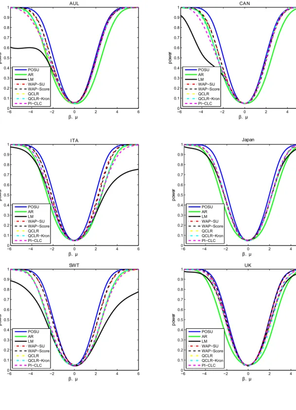
To assess the relative performance of all tests, we adopt parameter values estimated from Yogo (22, 2004) data, and we calibrate our simulations based on those values. Yogo considers estimation of elasticity of inter-temporal substitution in 11 developed countries using linear IV. Our design is similar to the one proposed by Andrews (5), but instead of using the real interest rate as the endogenous variable we use the real aggregate stock return. This modification is motivated by the fact that weak identification problem seems to affect more the estimation of the EIS when we use the real aggregate stock return as the endogenous variable7.
This design requires estimates forµand Ψ from equations 9 and 10. To obtain these estimates we calculate ˆµand ˆΨ based on two-stage least squares estimates for the EIS, where ˆΨ is a Newey-West covariance matrix estimator using three lags. The resulting power curves (based on 5.000 simulations) are plotted in figures 3-4
That is, for countryi we estimate ˆµi =T−1PZty2,t, take ˆβi to be the tow-sep GMM
estimate forβand let ˆΨilet the Newey-West covariance estimator forV ar
T−1P
ft( ˆβi)′, Zt′y2,t
based on 3 lags for all variables.
7
Figure 3: Simulations for Real Aggregate Stock Return as the Endogenous Variable
−6 −4 −2 0 2 4 6
0 0.1 0.2 0.3 0.4 0.5 0.6 0.7 0.8 0.9 1 β. µ po w er AUL POSU AR LM WAP−SU WAP−Score QCLR QCLR−Kron PI−CLC
−6 −4 −2 0 2 4 6
0 0.1 0.2 0.3 0.4 0.5 0.6 0.7 0.8 0.9 1 β. µ po w er CAN POSU AR LM WAP−SU WAP−Score QCLR QCLR−Kron PI−CLC
−6 −4 −2 0 2 4 6
0 0.1 0.2 0.3 0.4 0.5 0.6 0.7 0.8 0.9 1 β. µ po w er ITA POSU AR LM WAP−SU WAP−Score QCLR QCLR−Kron PI−CLC
−6 −4 −2 0 2 4 6
0 0.1 0.2 0.3 0.4 0.5 0.6 0.7 0.8 0.9 1 β. µ po w er Japan POSU AR LM WAP−SU WAP−Score QCLR QCLR−Kron PI−CLC
−6 −4 −2 0 2 4 6
0 0.1 0.2 0.3 0.4 0.5 0.6 0.7 0.8 0.9 1 β. µ po w er SWT POSU AR LM WAP−SU WAP−Score QCLR QCLR−Kron PI−CLC
−6 −4 −2 0 2 4 6
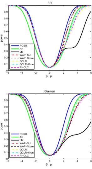
Figure 4: Simulations using Yogo data
−6 −4 −2 0 2 4 6
0 0.1 0.2 0.3 0.4 0.5 0.6 0.7 0.8 0.9 1 β. µ po w er NT H POSU AR LM WAP−SU WAP−Score QCLR QCLR−Kron PI−CLC
−6 −4 −2 0 2 4 6
0 0.1 0.2 0.3 0.4 0.5 0.6 0.7 0.8 0.9 1 β. µ po w er FR POSU AR LM WAP−SU WAP−Score QCLR QCLR−Kron PI−CLC
−6 −4 −2 0 2 4 6
11
Empirical Example
In this section we apply the different tests examined in this work to an empirical example. We use data from Yogo (22, 2004) to study the effect of weak instruments on the estimation of the elasticity of inter-temporal substitution.
For the estimation of the elasticity of inter-temporal substitution (EIS), we use quar-terly data8 on equity markets at an aggregate level and macroeconomic variables for eleven developed countries: Australia, Canada, France, Germany, Italy, Japan, Nether-lands, Sweden, Switzerland, United Kingdom and the United States. For each country, we estimate the EIS using two asset returns: the real interest rate, denoted by rf, and
the real aggregate stock return, denoted by re. The coefficient of interest is estimated
by
∆ct+1 =τi+ψri,t+1+ξi,t+1
The instruments used for the endogenous regressor ri,t+1 are the nominal interest
rate, inflation, consumption growth and log divident-price ratio. All instruments are lagged twice to avoid problems with time aggregation in consumption data.
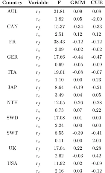
In table 1, we report the first-stage F-statistic for each of the possible endogenous regressors using TSLS estimates and assuming homoskedastic errors. We also report on the same table GMM and continuous updating estimator (CUE) of the EIS.
Unlike Yogo (2004) claim, we found that heteroskedasticity and autocorrelation have significant impact on inference.
It is worth noting that Score test have smaller confidence regions than WAP-LU test, despite the small number of instruments involved.
8
Table 1: Revisiting Yogo Results I
Country Variable F GMM CUE
AUL rf 21.81 0.09 0.08
re 1.82 0.05 -2.00 CAN rf 15.37 -0.34 -0.33
re 2.51 0.12 0.12
FR rf 38.43 -0.12 -0.12
re 3.09 -0.02 -0.02
GER rf 17.66 -0.44 -0.47 re 0.69 -0.05 -0.09
ITA rf 19.01 -0.08 -0.07
re 1.10 0.00 0.23
JAP rf 8.64 -0.19 -0.21
re 3.49 0.04 0.05
NTH rf 12.05 -0.26 -0.28
re 0.73 0.07 0.22
SWD rf 17.08 0.01 0.00
re 2.24 0.00 0.00
SWT rf 8.55 -0.39 -0.41
re 0.11 0.00 2.00
UK rf 17.04 0.22 0.28
re 2.62 -0.03 0.42
USA rf 11.92 0.02 -0.09
re [−∞,∞] [−∞,∞] [−∞,∞]
CAN rf [-0.54,-0.14] [−0.72,0.01]∪[3.90,14,15] [-0.74,0.03]
re [0.02,4.02] [-0.11,0.34] [-0.26,0.54]
FR rf [-0.67,0.52] [-0.46,0.31] [-0.47,0.31]
re [-0.27,0.20] [−∞,∞], [−∞,∞]
GER rf [-1.57,0.54] [-1.20,0.25]∪[11.30,16.01] [-1,24,0.28]
re [−∞,∞] [−∞,∞] [−∞,∞]
ITA rf [-0.29,0.18] [-6.51,-3.83]∪[−0.23,0.11] [-0.23,0.12]
re [−∞,∞] [−∞,∞] [−∞,∞]
JAP rf [-0.60,0.48] [−∞,−11.29]∪[-0.58,0.47]∪[6.16,∞] [0.56,0.45]
re [-0.04,0.32] [-1.00,0.20] [-∞,∞]
NTH rf [-0.90,0.64] [−∞,−17.21]∪[−0.77,0.48]∪[35.63,∞] [-0.79,0.52]
re [−∞,∞] [−∞,∞] [−∞,∞]
SWD rf [-0.30,0.28] [−0.20,0.20]∪[11.62,∞] [-0.22,0.21]
re [−∞,∞] [−∞,∞] [−∞,∞]
SWT rf [-1.68,0.34] [-1.19,0.07]∪[4.81,7,73] [-1.17,0.12]
re [−∞,∞] [−∞,∞] [−∞,∞]
UK rf [0.04,0.28] [−∞,−0.17]∪[−0.12,0.44]∪[7.22,∞] [-0.13,0.45]
re [-0.51,-0.02] [−∞,∞] [−∞,∞]
USA rf ∅ [−∞,27.93]∪[−0.28,0.27]∪[1,41,∞] [-0.28,0.28]
re [−∞,∞] [−∞,∞] [−∞,∞]
re [−∞,∞] [−∞,∞] [-0.19,0.13] [−∞,∞] [−∞,∞]
CAN rf [-0.76,0.10] [−∞,−8.82]∪[−1.02,0.34]∪[7.27,∞] ∅ [-0.86,0.20] [-0.84,0.17]
re [−∞,∞] [-0.12,0.72] [0.05,0.42] [−∞,∞] [−∞,∞]
FR rf [−0.56,0.35] [-0.39,0.16] [-0.34,0.12] [-0.39,0.17] [-0.39,0.17]
re [−∞,∞] [−∞,0.16] [-∞,−.12]∪[0.04,∞] [−∞,0.04]∪[0.25,∞] [−∞,0.04]∪[0.32,∞]
GER rf [-1.94,1.62] [−∞,−4.27]∪[−1.56,1.00]∪[3.81,∞] [−1,00,0.09]∪[11.85,14.68] [-1.60,1.54] [-1.59,1.20]
re [−∞,∞] [−∞,∞] [−∞,∞] [−∞,∞] [−∞,∞]
ITA rf [-0.34,0.20] [-∞,−1.37]∪[−0.25,0.11],[2.32,∞] [-0.18,0.04] [-0.26,0.11] [-0.25,0.10]
re [−∞,∞] [−∞,∞] [−∞,∞] [−∞,∞] [−∞,∞]
JAP rf [-0.92,0.39] [[-∞,−4.08]∪[−0.84,0.34]∪[1.67,∞] [-0.36,0.06] [-0.82,0.33] [-0.82,0.33]
re [−∞,∞] [−∞,∞] [0.00,0.15] [−∞,∞] [−∞,∞]
NTH rf [-0.56,0.08] [-∞,−2.38]∪[−0.83,4.7] ∅ [-0.73,1.82] [-0.70,1.67]
re [−∞,∞] [−∞,∞] [−∞,∞] [−∞,∞] [−∞,∞]
SWD rf [-0.28,0.28] [-∞,−8.05]∪[−0.20,0.20]∪[4.42,∞] [-0.11,0,10] [-0.20,0.22] [-0.20,0.20]
References
[1] Anderson, T. W., and H. Rubin (1949): “Estimation of the Parameters of a Single Equation in a Complete System of Stochastic Equations”,Annals of Mathematical Statistics, 20, 46–63.
[2] Andrews, D.W.K., Stock, J.H., (2006):“Inference with weak instruments”,Blundell, R., Newey, W.K., Persson, T. (Eds.), Advances in Economics and Econometrics, Theory and Applications: Ninth World Congress of the Econometric Society. Cam-bridge University Press, CamCam-bridge, UK.
[3] Andrews, D. W. K., M. J. Moreira, and J. H. Stock (2006):“Optimal Two-Sided Invariant Similar Tests for Instrumental Variables Regression”, Econometrica, 74, 715–752.
[4] Andrews, D. W. K., M. J. Moreira, and J. H. Stock (2006b): “Optimal Two-Sided Invariant Similar Tests for Instrumental Variables Regression”, Econometrica, 74, 715–752, Supplement.
[5] Andrews, I. (2014): “Combination Tests for Weakly Identified Models”, Unpub-lished Manuscript.
[6] Angrist, J., and A. B. Krueger (1991): “Does Compulsory School Attendance Affect Schooling and Earnings?,”The Quarterly Journal of Economics, 106, 979–1014.
[7] Campbell, John Y. (1998): “Data Appendix for ’Asset prices, Consumption and the Business Cycle’”, Unpublished Manuscript.
[8] Cragg, J.C., Donald, S.G., F. (1997): “Inferring the rank of a matrix ”,Journal of Econometrics , 76, 223250.
[9] Kleibergen, F. (2005): “Testing parameters in gmm without assuming they are identified”,Econometrica, 73, 11031123.
[10] Kleibergen, F. (2007): “Generalizing weak instrument robust IV statistics toward multiple parameters, unrestricted covariance matrices and identification statistics”,
Journal of Econometrics, 138, 181216.
[12] Moreira, M. J. (2002): “Tests with Correct Size in the Simultaneous Equations Model”, Ph.D. thesis, UC Berkeley.
[13] Moreira, M. (2003): “A conditional likelihood ratio test for structural models”,
Econometrica 71, 393410.
[14] Moreira, M. and Cruz, L. M. (2005): “On the validity of econometric techniques with weak instruments”,The Journal of Human Resources 71, 10271048.
[15] Moreira, M. J. (2009): “A Maximum Likelihood Method for the Incidental Param-eter Problem”,Annals of Statistics, 37, 3660–3696.
[16] Moreira, H. and Moreira, M. (2013): “Contributions to the theory of optimal tests”, Unpublished Manuscript.
[17] Moreira, H. and Moreira, M. (2013): “Contributions to the theory of optimal tests”, Unpublished Manuscript, Supplement.
[18] Staiger, D., and J. H. Stock (1997): “Instrumental Variables Regression with Weak Instruments,”Econometrica, 65, 557–586.
[19] Stock, J. and Wright, J. (2000): “Gmm with weak identification”, Econometrica
68, 10551096
[20] (2014): Vilela, L. “Generalized maxmin and minimax regret tests”, Unpublished Manuscript.
12
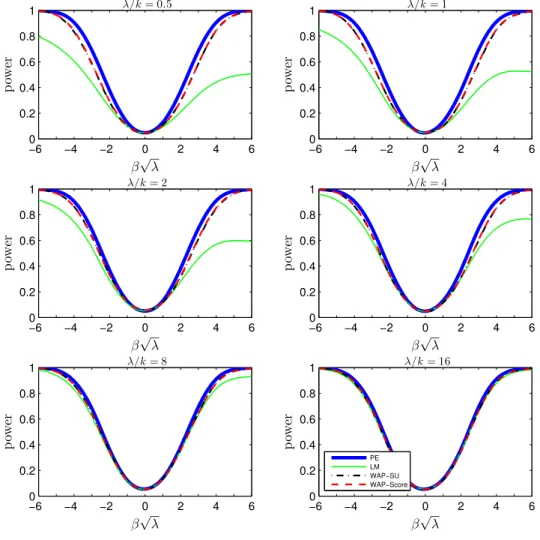
Appendix
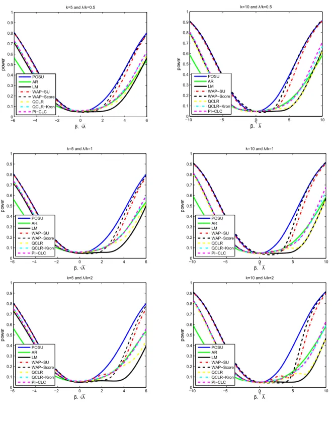
Figure 5: HACIV Power Comparison (Non-Kronecker Covariance): k= 2, ρ= 0.2
−6 −4 −2 0 2 4 6
0 0.2 0.4 0.6 0.8 1
β√λ
p
ow
er
λ/k= 0.5
−6 −4 −2 0 2 4 6
0 0.2 0.4 0.6 0.8 1
β√λ
p
ow
er
λ/k= 1
−6 −4 −2 0 2 4 6
0 0.2 0.4 0.6 0.8 1
β√λ
p
owe
r
λ/k= 2
−6 −4 −2 0 2 4 6
0 0.2 0.4 0.6 0.8 1
β√λ
p
owe
r
λ/k= 4
−6 −4 −2 0 2 4 6
0 0.2 0.4 0.6 0.8 1
β√λ
p
ow
er
λ/k= 8
−6 −4 −2 0 2 4 6
0 0.2 0.4 0.6 0.8 1
β√λ
p
ow
er
λ/k= 16
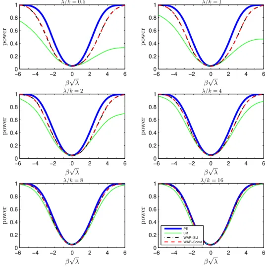
Figure 6: HACIV Power Comparison (Non-Kronecker Covariance): k= 2, ρ= 0.5
−6 −4 −2 0 2 4 6
0 0.2 0.4 0.6 0.8 1
β√λ
p
ow
er
λ/k= 0.5
−6 −4 −2 0 2 4 6
0 0.2 0.4 0.6 0.8 1
β√λ
p
ow
er
λ/k= 1
−6 −4 −2 0 2 4 6
0 0.2 0.4 0.6 0.8 1
β√λ
p
owe
r
λ/k= 2
−6 −4 −2 0 2 4 6
0 0.2 0.4 0.6 0.8 1
β√λ
p
owe
r
λ/k= 4
0.4 0.6 0.8 1 p owe r
λ/k= 8
0.4 0.6 0.8 1 p owe r
λ/k= 16
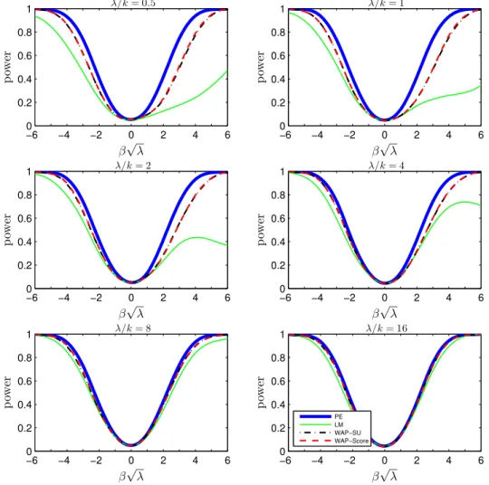
Figure 7: HACIV Power Comparison (Non-Kronecker Covariance): k= 2, ρ= 0.95
−6 −4 −2 0 2 4 6
0 0.2 0.4 0.6 0.8 1
β√λ
p
ow
er
λ/k= 0.5
−6 −4 −2 0 2 4 6
0 0.2 0.4 0.6 0.8 1
β√λ
p
ow
er
λ/k= 1
−6 −4 −2 0 2 4 6
0 0.2 0.4 0.6 0.8 1
β√λ
p
owe
r
λ/k= 2
−6 −4 −2 0 2 4 6
0 0.2 0.4 0.6 0.8 1
β√λ
p
owe
r
λ/k= 4
−6 −4 −2 0 2 4 6
0 0.2 0.4 0.6 0.8 1
β√λ
p
owe
r
λ/k= 8
−6 −4 −2 0 2 4 6
0 0.2 0.4 0.6 0.8 1
β√λ
p
owe
r
λ/k= 16
Figure 8: HACIV Power Comparison (Non-Kronecker Covariance): k= 5, ρ= 0.2
−6 −4 −2 0 2 4 6
0 0.2 0.4 0.6 0.8 1
β√λ
p
ow
er
λ/k= 0.5
−6 −4 −2 0 2 4 6
0 0.2 0.4 0.6 0.8 1
β√λ
p
ow
er
λ/k= 1
−6 −4 −2 0 2 4 6
0 0.2 0.4 0.6 0.8 1
β√λ
p
owe
r
λ/k= 2
−6 −4 −2 0 2 4 6
0 0.2 0.4 0.6 0.8 1
β√λ
p
owe
r
λ/k= 4
0.4 0.6 0.8 1 p owe r
λ/k= 8
0.4 0.6 0.8 1 p owe r
λ/k= 16
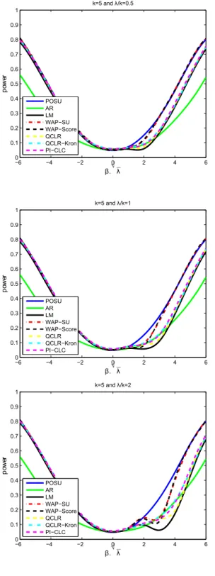
Figure 9: HACIV Power Comparison (Non-Kronecker Covariance): k= 5, ρ= 0.5
−6 −4 −2 0 2 4 6
0 0.2 0.4 0.6 0.8 1
β√λ
p
ow
er
λ/k= 0.5
−6 −4 −2 0 2 4 6
0 0.2 0.4 0.6 0.8 1
β√λ
p
ow
er
λ/k= 1
−6 −4 −2 0 2 4 6
0 0.2 0.4 0.6 0.8 1
β√λ
p
owe
r
λ/k= 2
−6 −4 −2 0 2 4 6
0 0.2 0.4 0.6 0.8 1
β√λ
p
owe
r
λ/k= 4
−6 −4 −2 0 2 4 6
0 0.2 0.4 0.6 0.8 1
β√λ
p
owe
r
λ/k= 8
−6 −4 −2 0 2 4 6
0 0.2 0.4 0.6 0.8 1
β√λ
p
owe
r
λ/k= 16
Figure 10: HACIV Power Comparison (Non-Kronecker Covariance): k= 5, ρ= 0.95
−6 −4 −2 0 2 4 6
0 0.2 0.4 0.6 0.8 1
β√λ
p
ow
er
λ/k= 0.5
−6 −4 −2 0 2 4 6
0 0.2 0.4 0.6 0.8 1
β√λ
p
ow
er
λ/k= 1
−6 −4 −2 0 2 4 6
0 0.2 0.4 0.6 0.8 1
β√λ
p
owe
r
λ/k= 2
−6 −4 −2 0 2 4 6
0 0.2 0.4 0.6 0.8 1
β√λ
p
owe
r
λ/k= 4
0.4 0.6 0.8 1 p owe r
λ/k= 8
0.4 0.6 0.8 1 p owe r
λ/k= 16
Figure 11: HACIV Power Comparison (Non-Kronecker Covariance): k= 10, ρ= 0.2
−6 −4 −2 0 2 4 6
0 0.2 0.4 0.6 0.8 1
β√λ
p
ow
er
λ/k= 0.5
−6 −4 −2 0 2 4 6
0 0.2 0.4 0.6 0.8 1
β√λ
p
ow
er
λ/k= 1
−6 −4 −2 0 2 4 6
0 0.2 0.4 0.6 0.8 1
β√λ
p
owe
r
λ/k= 2
−6 −4 −2 0 2 4 6
0 0.2 0.4 0.6 0.8 1
β√λ
p
owe
r
λ/k= 4
−6 −4 −2 0 2 4 6
0 0.2 0.4 0.6 0.8 1
β√λ
p
owe
r
λ/k= 8
−6 −4 −2 0 2 4 6
0 0.2 0.4 0.6 0.8 1
β√λ
p
owe
r
λ/k= 16
Figure 12: HACIV Power Comparison (Non-Kronecker Covariance): k= 10, ρ= 0.5
−6 −4 −2 0 2 4 6
0 0.2 0.4 0.6 0.8 1
β√λ
p
ow
er
λ/k= 0.5
−6 −4 −2 0 2 4 6
0 0.2 0.4 0.6 0.8 1
β√λ
p
ow
er
λ/k= 1
−6 −4 −2 0 2 4 6
0 0.2 0.4 0.6 0.8 1
β√λ
p
owe
r
λ/k= 2
−6 −4 −2 0 2 4 6
0 0.2 0.4 0.6 0.8 1
β√λ
p
owe
r
λ/k= 4
0.4 0.6 0.8 1 p owe r
λ/k= 8
0.4 0.6 0.8 1 p owe r
λ/k= 16
Figure 13: HACIV Power Comparison (Non-Kronecker Covariance): k= 10, ρ= 0.95
−6 −4 −2 0 2 4 6
0 0.2 0.4 0.6 0.8 1
β√λ
p
ow
er
λ/k= 0.5
−6 −4 −2 0 2 4 6
0 0.2 0.4 0.6 0.8 1
β√λ
p
ow
er
λ/k= 1
−6 −4 −2 0 2 4 6
0 0.2 0.4 0.6 0.8 1
β√λ
p
owe
r
λ/k= 2
−6 −4 −2 0 2 4 6
0 0.2 0.4 0.6 0.8 1
β√λ
p
owe
r
λ/k= 4
−6 −4 −2 0 2 4 6
0 0.2 0.4 0.6 0.8 1
β√λ
p
owe
r
λ/k= 8
−6 −4 −2 0 2 4 6
0 0.2 0.4 0.6 0.8 1
β√λ
p
owe
r
λ/k= 16
Figure 14: HACIV Power Comparison (Non-Kronecker Covariance): k= 20, ρ= 0.2
−6 −4 −2 0 2 4 6
0 0.2 0.4 0.6 0.8 1
β√λ
p
ow
er
λ/k= 0.5
−6 −4 −2 0 2 4 6
0 0.2 0.4 0.6 0.8 1
β√λ
p
ow
er
λ/k= 1
−6 −4 −2 0 2 4 6
0 0.2 0.4 0.6 0.8 1
β√λ
p
owe
r
λ/k= 2
−6 −4 −2 0 2 4 6
0 0.2 0.4 0.6 0.8 1
β√λ
p
owe
r
λ/k= 4
0.4 0.6 0.8 1 p owe r
λ/k= 8
0.4 0.6 0.8 1 p owe r
λ/k= 16
Figure 15: HACIV Power Comparison (Non-Kronecker Covariance): k= 20, ρ= 0.5
−6 −4 −2 0 2 4 6
0 0.2 0.4 0.6 0.8 1
β√λ
p
ow
er
λ/k= 0.5
−6 −4 −2 0 2 4 6
0 0.2 0.4 0.6 0.8 1
β√λ
p
ow
er
λ/k= 1
−6 −4 −2 0 2 4 6
0 0.2 0.4 0.6 0.8 1
β√λ
p
owe
r
λ/k= 2
−6 −4 −2 0 2 4 6
0 0.2 0.4 0.6 0.8 1
β√λ
p
owe
r
λ/k= 4
−6 −4 −2 0 2 4 6
0 0.2 0.4 0.6 0.8 1
β√λ
p
owe
r
λ/k= 8
−6 −4 −2 0 2 4 6
0 0.2 0.4 0.6 0.8 1
β√λ
p
owe
r
λ/k= 16
Figure 16: HACIV Power Comparison (Non-Kronecker Covariance): k= 20, ρ= 0.95
−6 −4 −2 0 2 4 6
0 0.2 0.4 0.6 0.8 1
β√λ
p
ow
er
λ/k= 0.5
−6 −4 −2 0 2 4 6
0 0.2 0.4 0.6 0.8 1
β√λ
p
ow
er
λ/k= 1
−6 −4 −2 0 2 4 6
0 0.2 0.4 0.6 0.8 1
β√λ
p
owe
r
λ/k= 2
−6 −4 −2 0 2 4 6
0 0.2 0.4 0.6 0.8 1
β√λ
p
owe
r
λ/k= 4
0.4 0.6 0.8 1 p owe r
λ/k= 8
0.4 0.6 0.8 1 p owe r
λ/k= 16
Figure 17: HACIV Power Comparison (Non-Kronecker Covariance): k= 50, ρ= 0.2
−8 −6 −4 −2 0 2 4−8 −6
0 0.2 0.4 0.6 0.8 1
β√λ
p
ow
er
λ/k= 0.5
−8 −6 −4 −2 0 2 4−8 −6
0 0.2 0.4 0.6 0.8 1
β√λ
p
ow
er
λ/k= 1
−8 −6 −4 −2 0 2 4−8 −6
0 0.2 0.4 0.6 0.8 1
β√λ
p
owe
r
λ/k= 2
−8 −6 −4 −2 0 2 4−8 −6
0 0.2 0.4 0.6 0.8 1
β√λ
p
owe
r
λ/k= 4
−8 −6 −4 −2 0 2 4−8 −6
0 0.2 0.4 0.6 0.8 1
β√λ
p
owe
r
λ/k= 8
−8 −6 −4 −2 0 2 4−8 −6
0 0.2 0.4 0.6 0.8 1
β√λ
p
owe
r
λ/k= 16
Figure 18: HACIV Power Comparison (Non-Kronecker Covariance): k= 50, ρ= 0.5
−8 −6 −4 −2 0 2 4−8 −6
0 0.2 0.4 0.6 0.8 1
β√λ
p
ow
er
λ/k= 0.5
−8 −6 −4 −2 0 2 4−8 −6
0 0.2 0.4 0.6 0.8 1
β√λ
p
ow
er
λ/k= 1
−8 −6 −4 −2 0 2 4−8 −6
0 0.2 0.4 0.6 0.8 1
β√λ
p
owe
r
λ/k= 2
−8 −6 −4 −2 0 2 4−8 −6
0 0.2 0.4 0.6 0.8 1
β√λ
p
owe
r
λ/k= 4
0.4 0.6 0.8 1 p owe r
λ/k= 8
0.4 0.6 0.8 1 p owe r
λ/k= 16
Figure 19: HACIV Power Comparison (Non-Kronecker Covariance): k= 50, ρ= 0.95
−8 −6 −4 −2 0 2 4−8 −6
0 0.2 0.4 0.6 0.8 1
β√λ
p
ow
er
λ/k= 0.5
−8 −6 −4 −2 0 2 4−8 −6
0 0.2 0.4 0.6 0.8 1
β√λ
p
ow
er
λ/k= 1
−8 −6 −4 −2 0 2 4−8 −6
0 0.2 0.4 0.6 0.8 1
β√λ
p
owe
r
λ/k= 2
−8 −6 −4 −2 0 2 4−8 −6
0 0.2 0.4 0.6 0.8 1
β√λ
p
owe
r
λ/k= 4
−8 −6 −4 −2 0 2 4−8 −6
0 0.2 0.4 0.6 0.8 1
β√λ
p
owe
r
λ/k= 8
−8 −6 −4 −2 0 2 4−8 −6
0 0.2 0.4 0.6 0.8 1
β√λ
p
owe
r
λ/k= 16