Convergence in Brazil: recent trends and long run prospects

...

' " .,...FUNDAÇÃO ' " OETUUO VARGAS EPGE

Escola de Pós-Graduação em Economia

SEMINÁRIOS

DE PESQUISA

ECONÔMICA

"Convergence in Brazil: Recent Trends and

Long Run Prospects"

--

.

Prof. Monso Ferreira (UFMG)

LOCAL

Fundação Getulio Vargas

Praia de Botafogo, 190 - 100 andar - Auditório

DATA 04/03/99 (5a _feira)

HORÁRIO 16:00h

...

--CONVERGENCE IN BRAZIL: RECENT

TRENDS AND LONG RUN PROSPECTS

V

Afonso Ferreira

Department 01 Economics, University 01 Minas Gerais (UFMG), Brazil

Abstract

This paper applies to the analysis of the interstate income distribution in BraziI a set of techniques that have been widely used in the current empirical literature on growth and convergence. Usual measures of dispersion in the interstate income distribution (the

coefficient of variation and Theil' s index) suggest that cr-convergence was an unequivoca1 feature of the regional growth experience in BraziI, between 1970 and 1986. After 1986, the process of convergence seems, however, to have sIowed down almost to a halt. A standard growth modeI is shown to fit the regional data well and to expIain a substantial amount of the

variation in growth rates, providing estimates of the speed of (conditional) J3-convergence of approximateIy 3% p.a .. Different estimates of the long run distribution implied by the recent growth trends point towards further reductions in the interstate income inequality, but also

suggest that the relative per capita incomes of a significant number of states and the number of ''very poor" and

, . . - - - -- - -

---•

Current address: 25 Wimpole Road - Beeston Nottingham NG9 3LQ United Kingdom; e-mail: afonsoferreira@compuserve.com.

1. INTRODUCTION

This paper applies to the analysis of the interstate income distribution in Brazil a set of

techniques that have been widely used in the current empirical literature on growth and

convergence. The recent trends in the interstate income distribution are analysed in Section 2,

while Section 3 presents the results of two exercises which attempt to detennine the long run

shape ofthe distribution implied by those trends. Some conclusions are suggested in Section 4.

2. RECENT TRENDS IN THE INTERSTATE INCOME DISTRIBUTION IN BRAZIL1

2.1 cr-Convemence

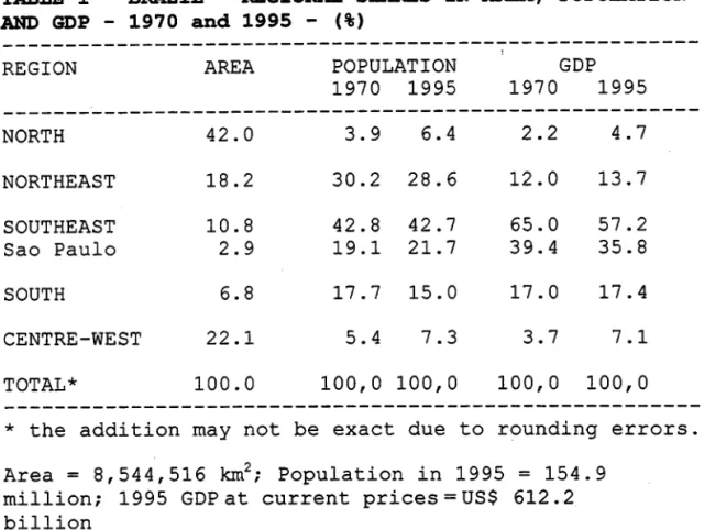
Economic activity in Brazil is concentrated in a relatively small portion of the territory.

In 1995, the four states located in the Southeast, which occupy together only 11 % of the

country's area, accounted for 43% ofthe population and·57% ofthe Brazilian GDP (Table 1).

More important, the differences in per capita incomes (PCIs) across states and regions

are significant. Brazil's per capita income, evaluated at the current exchange rate, amounted to

US$ 3 953, in 1995. The PCI of the richest state (Distrito Federal), at US$ 7 946, was two

times higher than the national mean and more than seven times higher than the per capita

income of the poorest state (US$ 1 067, in Piaui). While the per capita income of the

Northeast, the poorest region, was less than half the country's mean, the Southeast had a PCI

34% higher than the national average (Tables 2 and 3).

Although, as indicated above, spatial concentration is stiIl high, the geographical

ＮＭＭＭＭｾｾＭｾｾ＠ ＭＭＭＭｾＭＭＭＭＭＭＭＭｾＭＭＭＭＭＭＭｾＭＭＭＭＭＭ - - - --- - -- - - -ＭｾｾｾｾｾｾｾｾｾｾｾｾｾｾＭ

..

_.

-"

Southeast falling from 65% to 57%, while the shares of alI other regions, especially the North

and Centre-West, increased (Table 1).

Figure 1 shows that the dispersion of the state per capita incomes around the national

mean has also been reduced, in the past 25 years. The variables RATI070 and RATI095 in

that figure are the ratios ofthe state PCIs to the national mean, in 1970 and 1995, respectively,

ordered according to their 1970 values. As can be readily seen from Figure 1, for 20 of the 25

states, RATI095 is elo ser to 1 than RATI070.

The information regarding the differences in state per capita incomes, shown in Figure

1, can be summarised in a single measure of the degree of inequality in the interstate income

distribution - Theil's inequality index, given by:

(1)

where Pi

=

=

country's GDP, L

=

=

For a perfectly egalitarian income distribution, defined as the situation in which alI

states have the same per capita income, the value of Theil's index will be zero. While this is

the rninirnum value that can be tak.en by the index, there is no maximum value defined for it.

The estimated value of Theil's index for the Brazilian interstate income distribution in

1995 is 0.116, with the

inter-regional

the total inequality among the states and the intra-regional differences playing a relatively

ir ..

ｾＮ＠

Annual estimates of Theil's index, for the period 1970/1995, suggest that

0'-convergence, i.e. a reduction in the dispersion of the PCIs around the national mean, took

place among the Brazilian states, at a relatively fast speed, between 1975 and 1986. After

1986, this index still tends to decline, but now only at a very slow pace (Table 3)2.

Increased equality in the

inter-regional

capita incomes within the Southeast (31 %) together account for 92% of the reduction in the

Theil's index, between 1970 and 1995. The remaining 8% are e,q,lained by the reduction in

inequality which also occurred within the other four regions (Ferreira, 1998).

2.2 B-Convergence

An inverse relationship between the growth rates of the state per capita incomes and

the initial PCI leveIs, what has been termed ｾＭ｣ｯｮｶ･ｲｧ･ｮ｣･Ｌ＠ is a necessary (but not sufficient)

condition for O'-convergence. Figure 2 shows that, as already could be inferred from the results

presented in the previous section, ｾＭ｣ｯｮｶ･ｲｧ･ｮ｣･＠ can be observed among the Brazilian states,

in the period 1970/1995.

The equation for the straight line adjusted to the data in Figure 2 is shown as Equation

4.1, in Table 4, where GROWTH

=

between 1970 and 1995 and INPCI

=

1970 (measured in dollars of 1995).

The sign and statistical significance of the coefficient on the 1970 income leveIs

suggest the existence of (at least as a first approximation, unconditional or absolute) ｾﾭ

c.

the recent empiricalliterature, which, in general, has detected absolute ｾＭ｣ｯｮｶ･ｲｧ･ｮ｣･＠ within

sets of "more similar" economies, such as states or regions of the same country

(Sala-i-Martin, 1996).

The speed of convergence of 1.0%, implied by the value of the coefficient on INPCI,

however, is well below the estimates of Sala-i-Martin (1996) for the US states (2.1%), the

Japanese prefectures (1.9%) and 90 regions in Europe (1.5%)3.

The value of ｾ＠ increases substantially when other variables, which are usually assumed

to determine per capita income in the steady-state, are introduced in the convergence

regression. Steady-state per capita income depends on the steady-state leveI of labor

productivity and on the rate of participation in the labor force. Long run productivity,

following Mankiw, Romer and Weil (1992), is, in turn, presumed here to be determ.ined by the

rate ofinvestment, a mea:sure ofthe stock ofhuman capital (average schooling) and the rate of

growth of the labor force. Estimates of this standard specification for the per capita growth

equation are presented in Tables 4,5,6 and 7.

The equations in Tables 4, 5 and 6 are cross-section regressions, referring to the period

1970/1995 (Table 4) and to the sub-periods 1970/80 (Table 5) and 1980/95 (Table 6). The

equations in Table 7 are pooled time series cross-section regressions, estimated by pooling the

data used in the regressions in Tables 5 and 6.

In each of those equations, GROWTH and GEAP are the average annual rates of per

capita income growth and labour force growth, in the corresponding period of estimation. The

variables INVRATE, SCHOOL andPART, in Tables 5, 6 and 7, are initial year (Le. either

Ｎｾ＠

••

•

tb.e economicalIy active population (EAP) and tb.e rate of participation in tb.e Iabour force

(EAP/populationt.

In

investment in 1970 and 1980, while SCHOOL and PART carne from averaging tb.e

infonnation on schooling and tb.e rate of participation for tb.e years 1970, 1980 and 19955 •

FoIlowing Sachs and Wamer (1997), a non-linear reIationship between schooling and

growtb. was assumed in alI regressions. We expect a positive sign for tb.e coefficient on

SCHOOL and a nega tive sign for tb.e coefficient on SCHOOLSQ (= SCHOOL squared), so

that, otb.er things equal, growtb. wiIl be higher in states witb. an intennediate levei tb.an in states

witb. very low or very high (in Brazilian tenns) leveIs of schooling.

A time effect, consisting of a dummy variabIe, witb. a value of zero, in tb.e period

1970/80, and a value of 1, in tb.e period 1980/95, was added to tb.e pooIed regressions, in Table

7, to controI for tb.e substantial difference in tb.e macroeconomic environment between tb.e twO

periods (tb.e 1970s were tb.e years of tb.e Brazilian "miracIe", a decade during which tb.e

Brazilian GDP per capita increased by 82%, while tb.e post-1980 years can be characterized as

a period of acute macroeconomic instability and stagnation of per capita output6 ).

The pooIed regressions also incIuded an interaction tenn, allowing for a change in tb.e

coefficient of tb.e initial per capita income leveIs between tb.e two periods.

FinalIy, two dummy variabIes, for tb.e states of Amazonas and Amapa, witb. a value of

1 for tb.ose states in tb.e period 1970/80 and zero otb.erwise, were added to Equations 7.1-7.37_•

AlI RHS variables, with the exception of the dummies, entered tb.e regressions in log

fonn.

In

was

coefficients are t-statistics calculated from heterocedasticity-consistent standard errors, while

.-• ã

..

•

the figures in the rows Nonnality, W and RESET are p-values for Jarque-Beras's test of

nonnality of the residuals, White's heterocedasticity test and Ramsey's test of model

specification, respectively.

Because of lack of data on schooling, the state of Acre was not inc1uded in the

regressions. Given the idiosyncratic nature of employment and economic activity in its area

(which corresponds to Brasilia, the nation's capital), the Distrito Federal was also excluded

from the calculations.

The regressions, in Tables 4, 5, 6 and 7, explain a considerable proportion of the

variation in growth rates, in the different periods to which they refer. The cross-section

regressions in Table 4, for example, account for approximately three quarters of the variation

in growtb. rates, in the 25 years under analysis.

The coefficients on the RHS variables display, in general, the theoretically predicted

signs, the only exception here being. the coefficient on the rate of labour force growtb., in

Equation 6.2, which, however, is not significantly different from zero.

The value of the speed of conditional convergence implied by the coefficients on the

initial income leveIs varies widely, from around 3%, in the cross-section regressions referring

to the whole 1970/95 period (Equations 4.3-4.5) to more than 7%, in the estimates for the

1970s (Equations 5.2-5.4), but is always considerably higher than that derived from the

absolute convergence regressions (Equations 4.1, 4.2,5.1 and 6.1)8 .

The coefficients on the rate of investment and the rate of labour force growth are not

significantly different from zero, whenever a fuIl specification of the growth equation is

...

."

one of those two variables exc1uded from the RHS, the statistical significance of the

coefficient on the remaining variable, in some cases, becomes high enough to make it possible

to reject the null hypothesis of a value of zero for it, at the 10% leveI, in a one side t-test

(Equations 4.5,5.3, 7.2 and 7.3). A nega tive correlation between the two variables, which is a

possible explanation for these results, would seem to be consistent with the notion that capital

and labour move in opposite directions, when there are differences in labour productivity (and,

therefore, in per capita incomes) among regions ofthe same country.

The coefficients on the schooling variables, in Equations 4.3-4.5 and Equations

7.1-7.3, which give estimates for the whole períod under analysis, suggest that the effect of

education on growth reaches a maximum at an average leveI of schooling between 4 and 5

years (the highest leveI of average schooling, in 1995, was 7.45 years, in the state of Rio de

Janeiro).

The results obtained also indica te that, as expected, per capita income growth is

positively correlated with the rate of participation in the labour force.

The intercept dummy, in the pooled regressions in Table 7, has the expected negative

sign, confirming that, other things equal, growth rates tended to be lower in the post-1980

years than in the 1970s, due to the poor macroeconomic conditions prevailing in the former

período

The interaction term in those regressions has a positive sign, suggesting tb.at the states

were approaching their steady state leveIs of per capita income at a slower pace, after 1980

(Equations 7.1-7.3). A similar conc1usion is suggested by a comparison ofthe estimates ofthe

·

and less than 4%, for the post-1980 years). Absolute convergence, however, again according to

Tables 5 and 6 (Equations 5.1 and 6.1), was faster afier 1980 than in the 1970s.

An interpretation that reconciles these two seemingly contradictory results goes as

follows. In the 1970s, a decade of generally high rates of per capita income growth,

convergence was restricted mainly to the states located in the Southeast, South and Centre

West regions (on1y in 5 of the 15 states located in the North and Northeast, the poorest

regions, the per capita income gap with respect to the national average was reduced in this

period). Afier 1980, simultaneously to the dramatic reduction in growth rates, the speed of

convergence among the rich states decelerated, while the poor states, in the North and

Northeast, started to catch up. As a consequence of these different influences, the estimates of

the speed of absolute and conditional convergence moved in opposite directions, between the

two periods.

The results described in this section are, in general, consistent with the hypothesis of

conditional ｾＭ｣ｯｮｶ･ｲｧ･ｮ｣･Ｌ＠ i.e. with the notion that on1y states with similar structural

characteristics (here represented by the propensity to invest, the stock of human capital, the

rate of labor force growth and the rate of participation) converge to the same steady-state leveI

of per capita income. The main implications of these results for the convergence prospects in

Brazil will become clear in Section 3.

3. TIIE LONG RUN INTERSTATE INCOME DISTRIBUTION IN BRAZIL:

ＬＮＭＭＭＭＭＭＭＭＭＭＭＭＭＭＭＭＭＭＭＭＭＭＭＭｾＭＭＭＭＭＭＭＭＭＭ

••

•

What is the long run shape of the interstate income distribution implied by the

tendencies just described? What can we expect that distribution to be, in the steady state, given

the regional growth experience in Brazil, in the last 25 years?

Jones (1997) suggests that the long run distribution of income among a set of

economies can be inferred from the principie

01

to which an economy' s per capita income should grow at a rate proportional to the gap

between its current and steady state values. Naming the factor of proportionality as the "speed

of convergence", we have:

growth of state i' s relative per capita income = speed

of convergence x percentage gap to own steady state

where the relative per capita income is the ratio of state i' s' PCI to thehighest state PCI.

(2)

The expression in (2) constitutes the main pillar of the recent empírical literature on

conditional ｾＭ｣ｯｮｶ･ｲｧ･ｮ｣･＠ and has motivated a large volume of research, in which, as in the

previous section of this paper, econometrics has been employed to provide estimates of the

speed of convergence and to expIain differences in growth rates.

In

assumption regarding the speed of convergence, that expression could be used to calcula te the

distribution ofthe steady state (relative) per capita incomes.

The results of such an exercise, based on information avaiIable for the Brazilian states,

•

•

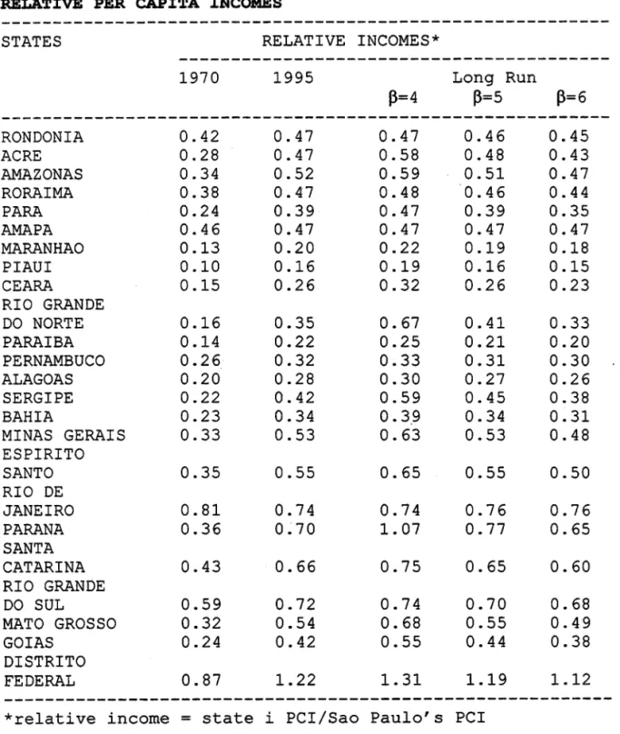
·-The first two columns in that table report the actual relative state per capita incomes

with respect to Sao Paulo (the largest and most successfu1:state economy), in 1970 and 1995 .

The Iong run estimates, shown in the Iast three columns, were derived from data on the relative

per capita income leveIs in 1970 and growth rates for the period 1970/1995, assuming values

for the speed of convergence of 4%, 5% and 6%.

When the speed of convergence is presumed to be 5%, the implied steady-state relative

per capita incomes are practically equal to the current (1995) relative PCIs and further gains

with respect to Sao Paulo are expected only for a very small group of states.

A value of

f3

moving toward leveIs ofrelative income, in the long run, lower than those reached in 1995, a

scenario that does not seem to be toa rea1istic.

A value of

f3

the prospects for a reduction in the gap between Sao Paulo and the other state economies, in

the Iong run. Note, however, that even in this case, for a non-negligible number of states,

including some ofthe poorest states in the Northeast, the predicted gains seem small (specially

when compared to those of the period 1970/95), which means that the current relative PCIs in

those states might be already quite close to their steady-state values.

Finally, values of the speed of convergence below 4% result in implausibly high

estimates of the long run relative per capita income for some states and are, therefore,

discarded (in this respect, see also Jones (1997)).

Are values of

f3

..

.

.

•

income leveIs in Equation 4.5, in Table 4, is equal to -2.528 (the value of that coefficient

which would correspond to an implied ｾ］ＴＥＩ＠ gives a p-value of 52%. Similar tests for the

cases of ｾ］ＵＥ＠ and ｾ］ＶＥ＠ result in p-values of 22% and 10%, respectively.

The estimates of the long run interstate income distribution derived from the

hypotheses of ｾ］ＴＥ＠ and ｾ］ＵＥ＠ not only seem to be consistent with the previous econometric

results but also constitute, at least in the context of the present exercise, the most intuitively

plausible interval in which the state PCIs may be expected to be found in the long run, given

the recent trends observed in the interstate distribution.

Another procedure that ean be used to "forecast" the shape of the long run ineome

distribution is based on Markov transition analysis and was first applied to the study of

eonvergenee by Quah (1993a, 1993b)9.

The Markov approaeh assumes that, given I possible ineome leveIs, each state has a

probability Pi(t) of being in leveI I at time t and a transition probability ID;j(t) of being in leveI j

at time t+l. Assuming, for simplicity, that the transition probabilities do not ehange over time

and ordering them as the Ix! transition matrix M, we get:

p(t+l) = p(t)M = p(O)M (3)

where p(t) is a Ix! row vector whose elements are the time-dependent probabilities Pi(t) and M

is the produet of t identieal M matrices .

W •

..

s=sM (4)

where s characterises the likely long run distribution of cross-state mcomes (European

Commission, 1997).

This approach has some advantages with respect to the conventional tests of ( j and

p-convergence adopted in Sections 2.1 and 2.2 as well as with respect to the exercise reported in

Table 8. First, itprovides information on what is happening to the entire cross-section of

(state) economies, i.e. it does not focus on any particular economy but on the shape of the

distribution as a whole (Quah, 1996; Jones, 1997). Second, "[it] provides evidence on

persistence and stratitication; on the formation of convergence clubs; and on the cross section

distribution polarising into twin peaks ofrich and poor" (Quah, 1996, pp. 1046Yo. Finally, it

does not assume that the states are growing toward constant targets, admitting, instead, shifts

in the steady state positions. In this sense, it provides a prediction of the very long run income

distribution (Jones, 1997).

To perform this exercise, I have assumed that, at any point in time, a state can be found

in one of the following tive situations, detined by its relative per capita income levei: "very

poor" (state PCI below 50% ofthe national mean); "poor" (state

pcr

the national mean); "medium" (state

pcr

"rich" (state PCI between 120% and 150% ofthe national mean); ''very rich" (state PCI above

150% ofthe national mean)ll .

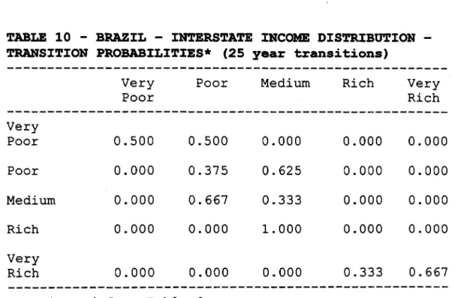
The Markov ana1ysis requires first the construction of the two way IxI cross-tabulation

4 •

and situationj in 199512_{• The second step is to derive, from the frequencies observed in Table}

9, the estimates ofthe ID;j transition probabilities that appear in Table 10.

In the period 1970/1995, a majority of states (fourteen in a total of twenty five) were

"movers". As shown in Table 9, five ofthe ''very poor" and five ofthe "poor" states, in 1970,

had moved to the immediately superior income category by 1995. Four states, on the other

hand, descended, in the per capita income ladder, to categories inferior to the ones in which

they found themselves in 1970. The other eleven states (among them, five ofthe ''very poor"

and two of the ''very rich" states, in 1970) were "stayers", remaining in the same situation

throughout.

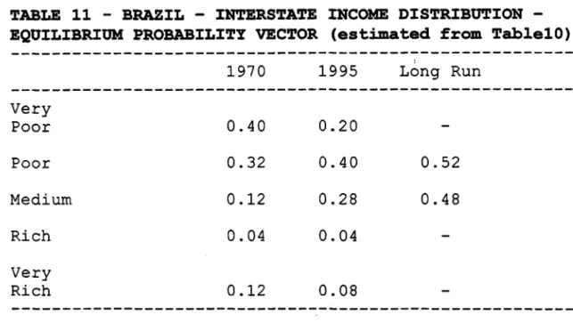
Using the transition probabilities in Table 10, the equilibrium probability vector,

giving the proportion of states at each of the five income leveIs in the stead.y state, was

estimated. The results are shown in Table 11, together with the 1970 and 1995 actual

distributions.

Table 11 suggests a tendency for the Brazilian states to move towards the middle

income categories. The proportion of "very poor" states, which fell from 40% to 20%, between

1970 and 1995, is predicted to become zero in the long run. Similarly, for the "very rich" and

"rich" states, the figures in Table 11 add up to 16%, in 1970, 12%, in 1995, and, again, zero, in

the steady state. The percentages of states in the "poor" and "medium" income intervals, in

turn, are expected to increase from 32% and 12%, in 1970, to 52% and 48%, respectively, in

the very long run. Although a substantial reduction in the interstate income inequality is

predicted by this exercise, absolute ｾＭ｣ｯｮｶ･ｲｧ･ｮ｣･＠ does not result, Le. the states are not

.

.

..

-An obvious flaw of the exercise reported in Tables 9-11 is the small number of

observations. The results in those tables were derived from data for the years 1970 and 1995

and, thus, refer to 25 year transitions. Tables 12-13 report the results of a similar exercise,

based on the 5 year transitions observed for the periods 1970/75, 1975/80, 1980/85, 1985/90

and 1990/95. The two exercises, thus, differ in two respects: the number of observations (25,

in the first case; 125, in the second) and the time horizon ofthe observed changes from which

the transitions matrices were derived (25 year changes and 5 year changes, respectively). A

third difference consists in that, in the second exercise, the "medium" income group was

partitioned in two different categories ("below the national average" and "above the national

average").

Comparing the entries in the main diagonals in Tables 10 and 12, we find, as expected,

higher persistence in the latter table than in the former. Both tables suggest a tendency for the

"very rich" and "rich" states to move toward lower leveIs of (relative) income and no tendency

for the states in the "medium" or lower (relative) income leveis to move in the opposite

direction (i.e. toward the "rich" and ''very rich" categories). Table 12, however, differs from

Table 10 in that there is a 5% probability for the "poor" and "below average" states to falI to

the ''very poor" income group.

As a consequence, while the long run distribution in Table 13, as that in Table 11, does

not display any ''very rich" and "rich" strata, it does contain a ''very poor" group of states. A

second distinctive feature ofthe results in Table 13 is that the expected proportions of states in

ＮＮＭＭＭＭＭＭｾＭＭ ｾＭＭｾＭＭｾＭＭＭＭＭＭＭ - -

-'"

.

,,-run distributions, in both tables, are, in any case, characterised by the same concentration of

states in the "poor" and "medium" income leveIs, i.e. by some degree of convergence.

4. CONCLUSIONS

The

roam

1) The usual measures of dispersion in the interstate income distribution

suggest that a-convergence was an unequivocal feature of the regional growth

experience in Brazil, between 1970 and 1986. The process of convergence seems,

however, to have slowed down almost to a halt, afier 1986.

2) A standard growth model, in which per capita income growth is assumed to

depend on the initial income leveI, the rate of investment, average schooling, the

rate of growth of the labour force and the rate of participation, explains a

substantial amount ofthe variation in growth rates in the period 1970/95. It should

be noted, however, that the performance of the model was not as satisfactory when

only data' for the 1980/95 years (a period characterised by Iow growth rates and

high economic instability) were used in its estimation.

3) The results of the growth regressions are consistent with the hypothesis of

conditional ｾＭ｣ｯｮｶ･ｲｧ･ｮ｣･Ｌ＠ the proposition that (only) states with similar structural

characteristics tend towards the same steady state per capita income leveI. As

predicted by the model, the rates of growth were found to vary directly with the

rate of investment, average schooling and the rate of participation and inversely

.'

relationship between schooling and per capita income growth is non-linear, with

intennediate leveIs of schooling having a highel' impact on growth than low or high

leveIs.

4) The point estimate for the speed of (conditional) convergence, when data

for the entire 1970/95 period were used in the estimation, was approximately 3%.

Conditional convergence seems to have been faster in the 1970s than after 1980.

5) Some evidence was found of a negative correlation between the rate of

investment and the rate of growth of the labour force, a result consistent with the

theoretical predictions regarding factor mobility, in the neoc1assical model.

6) Different estimates of the long run interstate income distribution pointed

7)

towards a tendency for the great majority of states to cluster in the interval between

50% and 120% ofthe national average (100% ofthe states, in Table 11, and 82%,

in Table 13 - against 44%, in 1970, and 68%; in 1995). Therefore, while we may

expect, on the basis of the trends observed between 1970 and 1995, further

reductions in the interstate income inequality, the data again do not support the

hypothesis of absolute f3-convergence.

Some exercises have suggested that the relative per capita incomes of a

significant number of states (Table 8) and the number of ''very poor" and "poor"

states (Table 13) were, in 1995, already quite c10se to their steady state values.

These results offer a possible explanation for the apparent weakening of the process

·

.

..

-NOTES

1. Previous work on the interstate income distribution in Brazil includes Azzoni (1994, 1996),

Ellery Jr. and Cavalcanti Ferreira (1994), Ferreira and Diniz (1995), Ferreira (1996) and

Ferreira (1998).

2.The coefficient of variation (standard deviation normalized by the mean) of the state PCIs

also fell, from 0.645, in 1970, to 0.462, in 1986, and increased slightly, afterwards, to reach a

leveI of 0.494, in 1995 (Table 3). The coefficient of variation is the measure of cr-convergence

most commonly adopted in the literature. I have, however, opted for emphasizing here the

results based on Theil' s index, because this index has the desirable feature of weighting the

(relative) state per capita incomes by the states' shares in the total population. In any case, the

evolution of the coefficient of variation was similar to that of the L index, during most of the

period under analysis.

3. The speed of convergence ｾ＠ can be inferred from the coefficient b in the regression

GROWTH

=

=

two observations used to estimate the average annual rates of growth, corresponding to 25

years, in this case (Sachs and Warner, 1997). Other country estimates ofthe speed ofabsolute

convergence reported in Sala-i-Martin (1996) are: Germany (1.4%), United Kingdom (2.0%),

w"

4. Direct infonnation on total investment at the state levei is not available. Data on industrial

investment (mining

+

proxy for total state investment, in those two years, was, thus, constructed by assuming that

the share of a state in the country's capital fonnation Was the same as its share in industrial

investment.

5. Mankiw, Romer and Weil (1992), among many others, also average the infonnation on the

right hand side (RHS) variables in their estimates of growth regressions. Endogeneity,

specially in relation to the rate ofinvestment, may, however, be a concem in this case. That is

one of the reasons why regressions using initial year values of the rate of investment,

schooling and the rate of participation, as welI as regressions in which the rate of investment

was exc1uded from the RHS, are also reported. The steady state levei of labor productivity

depends on the steady state levei of human capital, not on its initial period value or average

value during the period of estimation (Mankiw, Romerand Weil, 1992). To take this into

account, equations were estimated where final year values of SCHOOL were used (Islam,

1995). These latter results, which do not depart significant1y from those shown in Tables 4-7

are available from the author upon request.

6. The average annual rate ofper capita GDP growth felI from 6.6%, in the 1970s, to 0.1%, in

the period 1980/95. This context of low growth rates and high uncertainty and instability,

perhaps, explains why the perfonnance. of the model was, in general, less satisfactory, when

only data for the post-1980 years were used in its estimation (Equations 6.2-6.4).

7. Those were the states with, respectively, the highest (9.8%) and lowest (1.9%) rates ofper

."

Amazonas is explained by the creation of the Zona Franca de Manaus, a duty-free area

specialising mainly in the production of durable consumption goods (electrical appliances and

electronics) for the domestic market.

8. As it is well known, these bigher (conditional) values of ｾ＠ refer to the speed at wbich the

state PCIs are moving toward their own steady-state values, wbich may differ across states and

regions. What Islam (1995) observed with respect to the world income distribution also seems

to apply here: there may be little soIace to be derived from finding that the Brazilian states are

converging at a faster rate, if the points to wbich they are converging may remain very

different.

9. This technique has also been recently employed to determine the impact of the Single

Market Programme on the distribution of income and convergence among 169 regions in

Europe (European Commission, 1997) and adopted by Jones (1997) in bis study of the world

income distribution.

10. According to Quah, this is the main deficiency of the cr-convergence tests: on the basis of

such tests, it is not possible to uncover intra-distribution movements, the existence of

convergence clubs, ''twin-peaks dynamics" etc. With respect to the ｾＭ｣ｯｮｶ･ｲｧ･ｮ｣･＠ tests, Quah

argues that ''the cross-section correlation between growth rates and income leveIs revea1s even

less, its interpretation being plagued by a version of Galton's Fallacy" (Quah, 1996 and also

1993b).

11. Since the per capita incomes of even the richest states in Brazil are well below those of the

developed countries, the notions of "rich" and "very rich" adopted here, obviously, only make

sense when related to the Brazilian contexto

-

.

.,.

.

ｾ＠

.

..

-REFERENCES

Azzoni, Carlos (1994). Crescimento econômico e convergência das rendas regionais: o caso brasileiro, Anais do

XXIr

A.zzoni, Carlos (1996). Economic growth and regional income inequalities in Brazil (1939-1992), University of Sao Paulo, mimeo.

European Commission (1997). Regional growth and convergence, The Single Market Review,

subseries VI, vol. 1. Office for Official Publications of the European CommunitieslK.ogan Page-Earthscan.

Ellezy Jr., Roberto and Pedro Cavalcanti Ferreira (1994). Crescimento econômico e convergência entre as rendas dos estados brasileiros, Anais do XVIo Encontro Brasileiro de Econometria (SBE), pp. 264-286.

Ferreira, Afonso and Clelio Diniz (1995). Convergência entre as rendas per capita estaduais no Brasil, Revista de Economia Política 15(4), pp. 38-56.

Ferreira, Afonso (1996). A distribuição interestadual da renda no Brasil (1950-85), Revista Brasileira de _Economia 50(4), pp. 469-485.

Ferreira, Afonso (1998). Evolucao recente das rendas per capita estaduais no Brasil, Revista de Economia Politica 18(1), pp. 90-97.

Islam, Nazrul (1995). Growth empirics: a panel data approach, Quarterly Journal of Economics 110, pp. 1127-1170.

Jones, Charles (1997). On the evolution ofthe world income distribution, Journal ofEconomic Perspectives 11(3), pp. 19-36.

Mankiw, N. D. Romer and D. Weil (1992). A contribution to the empirics of economic growth, QuarterlyJournal ofEconomics 107(2), pp. 407-437.

Quah, Danny. (1993a). Empirical cross-section dynamics in economic growth, European Economic Review 37, pp. 426-434.

Quah, Danny (1993b). Galton's fallacy and tests ofthe convergence hypothesis, Scandinavian Journal ofEconomics 95(4), pp. 427-443.

Quah, D. (1996). Twin peaks: growth and convergence in models of distribution dynamics,

,,"

Sachs, Jeffrey and Andrew Warner (1997). Fundamental sources of long run growth, American Economic Review 87(2), pp. ＱＸＴｾＱＸＸＮ＠

ｓ｡ｬ｡ｾｩｾｍ｡ｲｴｩｮＬ＠ Xavier. (1996). The c1assical approach to convergence ana1ysis, Economic

."

TABLE 1 - BRAZIL - REGIONAL SUARES IN AREA, POPOLATION AND GDP - 1970 and 1995 - (%)

---REGION ARE A POPULATION

1970 1995

GDP 1970 1995

---NORTH 42.0 3.9 6.4 2.2 4.7

NORTHEAST 18.2 30.2 28.6 12.0 13.7

SOUTHEAST 10.8 42.8 42.7 65.0 57.2 Sao Paulo 2.9 19.1 21.7 39.4 35.8

SOUTH 6.8 17.7 15.0 17.0 17.4

CENTRE-WEST 22.1 5.4 7.3 3.7 7.1

TOTAL* 100.0 100,0 100,0 100,0 100,0

---* the addition may not be exact due to rounding errors.

Area = 8,544,516 km2; Population in 1995 = 154.9

mil1ion; 1995 GDP at current prices = US$ 612.2

billion

TABLE 2 - BRAZIL - REGIONAL GDP PER CAPITA RELATIVE TO TBE NATIONAL AVERAGE

REGION 1970 1995

---NORTH 0.58 0.72

NORTHEAST 0.40 0.48

Piaui 0.21 0.27

SOUTHEAST 1.52 1. 34

Rio de Janeiro 1. 66 1.22

Sao Paulo 2.06 1. 65

SOUTH 0.96 1.16

CENTRE-WEST 0.68 0.97

Distrito Federal 1. 79 2.01

OI' •

.-TABLE 3 - BRAZIL - INTERSTATE INCOME DISTRIBOTION - 1970/1995

YEAR Theil's Index

1970 0.216

1975 0.203

1980 0.164

1985 0.128

1986 0.119

1987 0.122

1988 0.123

1989 0.120

1990 0.119

1991 0.117

1992 0.119

1993 0.116

1994 0.111

1995 0.116

Coefficient of variation (standard deviation/ mean) 0.645 0.662 0.564 0.494 0.462 0.471 0.485 0.504 0.488 0.475 0.483 0.483 0.480 0.494 Richest State PCI*/ Poorest State PCI+

9.75 8.90 8.44 7.04 6.33 6.57 7.03 8.21 7.16 7.37 7.56 7.12 6.99 7.38

...

.

.

TABLE 4 - BRAZIL - TESTS OF ｾＭｃｏｎｖｅｒｇｅｎｃｅ＠ - CROSSSECTION RESULTS -1970/95 (dependent variable

=

RHS VARIABLES Eq.4.1 Eq.4.2 Eq.4.3 Eq.4.4 Eq.4.5

ＭＭＭＭＭＭＭＭＭＭＭＭＭＭＭＭＭＭＭＭＭＭＭＭＭＭＭＭＭＭＭＭＭＭＭＭＭＭＭＭＭＭＭＭＭＭＭＭＭＭＭｾＭＭ ＭＭＭＭＭＭＭＭＭＭＭＭＭ

Constant INPCI I NVRATE SCHOOL SCHOOLSQ GEAP PART

number of

9.790 (5.803)

-0.904 (-3.784)

1.024

observations 25

Adjusted R2 0.363

Normality 0.453

W 0.674

RESET 0.208

10.568 (6.366) -1. 021 (-4.370) 1.179 23 0.410 0.467 0.849 0.104 -9.579 (-1. 769) -2.048 (-3.168) 0.153 (0.512) 13.227 (2.869) -4.525 (-2.206) -0.268 (-0.427) 5.038 (3.146) 2.869 23 0.718 0.819 0.558 0.747 -9.062 (-1. 729) -1. 953 (-3.670) 14.208 (4.733) -4.931 (-3.545) -0.408 (-0.960) 4.733 (3.446) 2.679 23 0.731 0.586 0.533 0.811 -10.656 (-1.800) -2.172 (-4.029) 0.261 (1.491) 12.028 (4.599) -4.026 (-3.207) 5.573 (4.617 ) 3.133 23 0.729 0.961 0.553 0.631

Defini tion of the variables: GROWTH

=

capita income growth (1970/95); INPCI

=

1970; INVRATE

=

SCHOOL

=

=

average annual rate of growth of the labour force (1970/1995); PART

=

""

.

,,"

.,

-.

•

TABLE 5 - BRAZIL - TESTS OF ｾＭｃｏｎｖｅｒｇｅｎｃｅ＠ - CROSSSECTION RESULTS -1970/80 (dependent variable

=

---RHS VARIABLES Eq.5.1 Eq.5.2 Eq.5.3 Eq.5.4

---Constant 12.763 -16.555 -14.468 -19.737

(3.554) (-0.911) (-0.835) (-1.258)

INPCI -0.826 -5.360 -5.153 -5.867

(-1.561) (-2.613) (-2.893) (-3.317)

I NVRATE 0.277 0.562

(0.454) (1.234)

SCHOOL 14.321 14.957 13.464

(4.610) (5.513) (4.848)

SCHOOLSQ -5.673 -6.018 -5.102

(-3.050) (-4.242) (-3.223)

GEAP -0.733 -1. 034

(-0.736) (-1. 480)

PART 16.191 15.423 17.727

(2.036) (2.113) (2.709)

ｾ＠ 0.862 7.678 7.243 8.836

number of

observations 23 23 23 23

Adjusted R2 _{0.014 0.402 0.431 0.423}

Normality 0.709 0.310 0.473 0.219

W 0.164 0.763 0.605 0.718

RESET 0.310 0.107 0.097 0.261

Defini tion of the variables: GROWTH

=

capita income growth; INPCI

=

year; INVRATE

=

=

years of schooling in the initial year; GEAP

=

growth of the labour force; PART

=

....

.,

-.

-•

TABLE 6 - BRAZIL - TESTS OF ｾＭｃｏｎｖｅｒｇｅｎｃｅ＠ - CROSSSECTION RESULTS -1980/95 (dependent variable

=

RHS VARIABLES

Constant INPCI INVRATE SCHOOL SCHOOLSQ GEAP PART SERGIPE

ｾ＠

Number of Observations

Adjusted R2

Normality W RESET Eq.6.1 11.546 (5.977) -1. 363 (-5.660) 1.524 23 0.496 0.042 0.616 0.309 Eq.6.2 7.588 (0.978) -2.940 (-3.479) 0.260 (0.514) 7.101 (1.667) -1. 933 (-1. 063) 0.558 (0.891) 2.557 (1.064) 3.877 23 0.507 0.004 0.981 0.562 Eq.6.3 13.658 (3.691) -2.316 (-4.220) 7.175 (2.872) -2.195 (-2.104) 2.844 23 0.555 0.008 0.782 0.397 Eq.6.4 13.470 (3.799) -2.232 (-4.291) 6.107 (2.459) -1.724 (-1. 679) 2.145 (13.522) 2.718 23 0.744 0.416 0.929 0.479

....

""

"

.

.'

TABLE 7 - BRAZIL - TESTS OF ｾＭｃｏｎｖｅｒｇｅｎｃｅ＠ - POOLED ESTIMATION -1970/95 (dependent variable

=

---RHS VARIABLES Eq.7.1 Eq.7.2 Eq.7.'3

---Constant 15.602 13.937 17.400

(1.421) (1.314) (1.854)

DUMMY -13.738 -13.929 -14.087

(-3.856) (-3.873) (-4.149)

INPCI -4.235 -4.497 -3.848

(-6.547) (-5.992) (-6.102)

DUMMY* 1.062 1.082 1.114

INPCI (2.371) (2.401) (2.601)

I NVRATE 0.422 0.550

(1. 016) (1.431)

SCHOOL 9.666 9.214 10.695

(4.340) (4.584) (5.915)

SCHOOLSQ -3.129 -2.853 -3.776

(-2.636) (-2.609) (-4.118)

GEAP -0.366 -0.785

(-0.639) (-1. 427)

PART 4.610 5.429 3.696

(1.328) (1. 606) (1.274)

Number of

Observations 46 46 46

Adjusted R2 _{0.922 0.923 0.921}

Normality 0.815 0.853 0.817

W '0.582 0.288 0.533

RESET 0.694 0.684 0.581

Defini tion of the variables: GROWTH = average annual rate of per capi ta

income growth in 1970/80 and 1980/95; INPCI = per capita income levels in

1970 and 1980; INVRATE = rate of investment in 1970 and 1980; SCHOOL = years

of schooling in 1970 and 1980; GEAP = average annual rate of growth of the

labour force in 1970/80 and 1980/95; PART = rate of participation in 1970

and 1980; DUMMY

=

...

.

."

-••

TABLE 8 - BRAZIL - LONG RON ESTlMATES OF TBE STATES RELATlVE PER CAPITA INCOMES

STATES RELATIVE INCOMES*

1970 1995 Long Run

(3=4

(3=5

(3=6

RONDONIA ACRE AMAZONAS RORAIMA PARA AMAPA MARANHAO PIAUI CEARA

RIO GRANDE DO NORTE PARAIBA PERNAMBUCO ALAGOAS SERGIPE BAHIA

MINAS GERAIS ESPIRITO SANTO RIO DE JANEIRO PARANA SANTA CATARINA RIO GRANDE DO SUL

MATO GROSSO GOlAS DISTRITO FEDERAL 0.42 0.28 0.34 0.38 0.24 0.46 0.13 0.10 0.15 0.16 0.14 0.26 0.20 0.22 0.23 0.33 0.35 0.81 0.36 0.43 0.59 0.32 0.24 0.87 0.47 0.47 0.52 0.47 0.39 0.47 0.20 0.16 0.26 0.35 0.22 0.32 0.28 0.42 0.34 0.53 0.55 0.74 0.70 0.66 0.72 0.54 0.42 1.22 0.47 0.58 0.59 0.48 0.47 0.47 0.22 0.19 0.32 0.67 0.25 0.33 0.30 0.59 0.3,9 0.63 0.65 0.74 1. 07 0.75 0.74 0.68 0.55 1. 31 0.46 0.48 0.51 0.46 0.39 0.47 0.19 0.16 0.26 0.41 0.21 0.31 0.27 0.45 0.34 0.53 0.55 0.76 0.77 0.65 0.70 0.55 0.44 1.19

*relative income

=

...

.

ｾ＠

••

TABLE 9 - BRAZXL - CROSS-TABULATXON OF TBE STATES ACCORDXNG TO TBEXR GDP PER CAPXTA RELATXVE TO TBE NATXONAL AVERAGE -1970 and 1995

Very Poor

Poor

1970 Medium

Rich Very Rich Very Poor 5 1995

Poor Medium Rich

5

3 5

2 1

1

1

TABLE 10 - BRAZXL - XNTERSTATE INCOME DXSTRIBUTXON -TRANSXTXON PROBABXLXTXES* (25 year transitions)

Very Poor Poor Medium Rich Very Rich Very Poor 0.500 0.000 0.000 0.000 0.000 Poor 0.500 0.375 0.667 0.000 0.000

Medium Rich

0.000 0.000

0.625 0.000

0.333 0.000

1. 000 0.000

0.000 0.333

Very Rich 0.000 0.000 0.000 0.000 0.667 Very Rich 2

---*

-...

"

.

••

TABLE 11 - BRAZIL - INTERSTATE INCOME DISTRIBUTION -EQUILIBRIOM PROBABILITY VECTOR (estimated from Table10)

1970 1995 Long Run

Very

Poor 0.40 0.20

Poor 0.32 0.40 0.52

Medium 0.12 0.28 0.48

Rich 0.04 0.04

Very

Rich 0.12 0.08

TABLE 12 - BRAZIL - INTERSTATE INCOME DISTRIBUTION -TRANSITION PROBABILITIES (5 year transitions)

Poor Very Poor Poor Below Average Above Average Rich Very Rich Very 0.805 0.051 0.053 0.000 0.000 0.000 Poor 0.195 0.718 0.263 0.000 0.000 Below Average 0.000 0.231 0.474 0.400 0.000

0.000 0.000

Above Rich Very Rich Average

0.000 0.000 0.000

0.000 0.000 0.000

0.210 0.000 0.000

0.600 0.000 0.000

0.143 0.857 0.000

0.000 0.083 0.917

number of transitions with starting points in each income

ＮＮＬＮＮＢＮＮＬＭｾＭＭＭＭＭＭｾＭＭＭＭＭＭＭＭｾＭＭＭＭＭ --- --- - - - -ＭＭＭＭＭＭＭＭＭＭＭＭＭＭＭｾ＠

"

.

-•

TABLE 13 - BRAZIL - INTERSTATE INCOME DISTRIBUTION -EQOILIBRIUM PROBABILITY VECTOR Ｈ･ｳｴｾｴ･､＠ from Tab1e 12)

Very Poor

Poor

Below Average

Above Average

Rich

Very Rich

1970

0.40

0.32

0.12

0.04

0.12

1995 Long Run

0.20 0.18

0.40 0.39

0.16 0.28

0.12 0.15

0.04

...

...

•

FIGURE 1

ＲＮＵｾ＠

________________________________

2.0

1.5

1.0

0.5

·

_·

_·

_·

·

_·

_·

_·

·

_·

_·

_·

·

_·

.

ｾ＠

.

\ /\

"

ＭＭＭＭＭＭＭｾ＠ \ ＭｦｾＭＭＭＭｩＭＭｾＭＭＭＭＭＭＭＭＭＭＭＭＭＭＭＭＭＭＭＭＭＭＭＭＭＭＭＭＭＭＭＭＭＭＭＭ \ ' \

'\,' , ,/ ... _ ...

-

-

• '

..

2 4

6

8 10 12 14 16 18 20 22 24

...

ｾ＠

5

.JI"

+

+

+

4

+

+

+ +

+

++

+

₊

₊

:r:

+

.-

₊

ｾ＠

3

+

O

_o::

+

+

C)

+

2

+

₊

+

1

6.0

6.5

7.0

.7.5

8.0

8.5

, I

!

N.Cham. P/EPGE SPE F383c

Autor: Ferreira, Afonso Henrique Borges

Título: Convergence in Brazil : recent trends and long run

1111111111111111111111111111111111111111

ｾＺｯｾｾＸＸ＠

FGV -BMHS N° Pat.: F2423/99

000088988