DAE Tools: equation-based object-oriented
modelling, simulation and optimisation
software
Dragan D. Nikolic1,2 1DAE Tools Project, Belgrade, Serbia
2MABE, Faculty of Science & Engineering, University of Limerick, Limerick, Ireland
ABSTRACT
In this work, DAE Tools modelling, simulation and optimisation software, its programming paradigms and main features are presented. The current approaches to mathematical modelling such as the use of modelling languages and general-purpose programming languages are analysed. The common set of capabilities required by the typical simulation software are discussed, and the shortcomings of the current approaches recognised. A new hybrid approach is introduced, and the modelling languages and the hybrid approach are compared in terms of the grammar, compiler, parser and interpreter requirements, maintainability and portability. The most important characteristics of the new approach are discussed, such as: (1) support for the runtime model generation; (2) support for the runtime simulation set-up; (3) support for complex runtime operating procedures; (4) interoperability with the third party software packages (i.e. NumPy/SciPy); (5) suitability for embedding and use as a web application or software as a service; and (6) code-generation, model exchange and co-simulation capabilities. The benefits of an equation-based approach to modelling, implemented in a fourth generation object-oriented general purpose programming language such as Python are discussed. The architecture and the software implementation details as well as the type of problems that can be solved using DAE Tools software are described. Finally, some applications of the software at different levels of abstraction are presented, and its embedding capabilities and suitability for use as a software as a service is demonstrated.
Subjects Scientific Computing and Simulation
Keywords Modelling, Simulation, Optimisation, Modelling languages, Model exchange, Domain specific languages, Equation-based, DAE, Code generation
INTRODUCTION
In general, two main approaches to mathematical modelling currently exist: (a) use of modelling languages, either domain specific or multi-domain such as Modelica (Fritzson & Engelson, 1998), Ascend (Piela et al., 1991), gPROMS (Barton & Pantelides, 1994), GAMS (Brook, Kendrick & Meeraus, 1988), Dymola (Elmqvist, 1978), APMonitor (Hedengren et al., 2014), and (b) use of general-purpose programming languages, either lower level third-generation languages such as C, C++ and Fortran (i.e. PETSc–a suite of data structures and routines for the scalable solution of scientific applications,Balay et al., 2015, and SUNDIALS–Suite of Nonlinear and Differential/Algebraic Equation Solvers, Hindmarsh et al., 2005), or higher level fourth-generation languages such as Python (i.e. Assimulo–a high-level interface for a wide variety of ODE/DAE solvers Submitted5 December 2015
Accepted7 March 2016
Published6 April 2016
Corresponding author Dragan D. Nikolic, dnikolic@daetools.com
Academic editor Linda Petzold
Additional Information and Declarations can be found on page 26
DOI10.7717/peerj-cs.54
Copyright 2016 Nikolic
Distributed under
written in C and Fortran, Andersson, Fuhrer & Akesson, 2015) and multi-paradigm numerical languages: MATLAB (MathWorks, Inc., 2015), Mathematica (Wolfram Research, Inc., 2015), Maple (Waterloo Maple, Inc., 2015), Scilab (Scilab Enterprises, 2015), and GNU Octave (Eaton et al., 2015). The lower-level general purpose languages are also often used for the development of the efficient, tailor-made software (i.e. large-scale finite difference and finite element solvers) targeting one of the available high-performance computing architectures such as General Purpose Graphics Processing Units (GPGPU), Field-Programmable Gate Arrays (FPGA), vector processors and Data Flow Engines (DFE). In addition, some modelling tools provide the Python scripting interface to the simulator engine: APMonitor, JModelica (Akesson et al., 2010), and OpenModelica (Fritzson et al., 2005); however, their API is limited to the loading of developed models, execution of simulations and processing of the results only. Domain Specific Languages (DSL) are special-purpose programming or specification languages dedicated to a particular problem domain and directly support the key concepts necessary to describe the underlying problems. They are created specifically to solve problems in a particular domain and usually not intended to be able to solve problems outside it (although that may be technically possible in some cases). More versatile, multi-domain modelling languages (such as Modelica or gPROMS) are capable of solving problems in different application domains. Despite their versatility, modelling languages commonly lack or have a limited access to the operating system, third-party numerical libraries and other capabilities that characterise full-featured programming languages, scripting or otherwise. In contrast, general-purpose languages are created to solve problems in a wide variety of application domains, do not support concepts from any domain, and have a direct access to the operating system, low-level functions and third-party libraries.
The most important tasks required to solve a typical simulation or optimisation problem include: the model specification, the simulation setup, the simulation execution, the numerical solution of the system of algebraic/differential equations, and the
functionality. Finally, the current trends in IT industry show that there is a high demand for cloud solutions, such as Software as a Service (SaaS), Platform as a Service (PaaS) and web applications.
A modelling language implemented as a single monolithic software package can rarely deliver all capabilities required. For instance, the Modelica modelling language allows calls to “C” functions from external shared libraries but with some additional pre-processing. Simple operating procedures are supported directly by the language but they must be embedded into a model, rather than separated into an independent section or function. gPROMS also allows very simple operating procedures to be defined as tasks (only in simulation mode), and user-defined output channels for custom processing of the results. The runtime model generation and complex operating procedures are not supported. Invocation from other software is either not possible or requires an additional application layer. On the other hand, Python, MATLAB and the software suites such as PETSc have an access to an immense number of scientific software libraries, support runtime model generation, completely flexible operating procedures and processing of the results. However, the procedural nature and lack of object-oriented features in MATLAB and absence of fundamental modelling concepts in all three types of environments make development of complex models or model hierarchies difficult.
In this work, a new approach has been proposed and implemented in DAE Tools software which offers some of the key advantages of the modelling languages coupled with the power and flexibility of the general-purpose languages. It is a type of hybrid approach–it is implemented using the general-purpose programming languages such as C++ and Python, but provides the Application Programming Interface (API) that resembles a syntax of modelling languages as much as possible and takes advantage of the higher level general purpose languages to offer an access to the operating system, low-level functions and large number of numerical libraries to solve various numerical problems. To illustrate the new concept, the comparison between Modelica and gPROMS grammar and DAE Tools API for a very simple dynamical model is given in theSource Code Listings 1–3, respectively. The model represents a cylindrical tank containing a liquid inside with an inlet and an outlet flow where the outlet flowrate depends on the liquid level in the tank. It can be observed that the DAE Tools API mimics the expressiveness of the grammar of modelling languages to provide the key modelling concepts while retaining the full power of general purpose programming languages. More details about the API is given in the sectionArchitecture.
Listing 1 Buffer Tank model (Modelica)
modelBufferTank
// Import libs
importModelica.Math.*;
parameter RealDensity;
parameter RealCrossSectionalArea;
RealHoldUp(start = 0.0);
RealFlowIn;
RealFlowOut;
RealHeight;
equation
// Mass balance
der(HoldUp) = FlowIn-FlowOut;
// Relation between liquid level and holdup
HoldUp = CrossSectionalArea * Height * Density;
// Outlet flowrate as a function of the liquid level
FlowOut = Alpha * sqrt(Height);
endBufferTank;
Listing 2 Buffer Tank model (gPROMS)
PARAMETER
Density AS Real
CrossSectionalArea AS Real
Alpha AS Real
VARIABLE
HoldUp AS Mass FlowIn AS Flowrate FlowOut AS Flowrate Height AS Length
EQUATION
# Mass balance
$HoldUp = FlowIn-FlowOut;
# Relation between liquid level and holdup
HoldUp = CrossSectionalArea * Height * Density;
# Outlet flowrate as a function of the liquid level
FlowOut = Alpha * sqrt(Height);
Listing 3 Buffer Tank model (DAE Tools)
classBufferTank(daeModel):
def__init__(self, Name, Parent = None, Description =""): daeModel.__init__(self, Name, Parent, Description)
self.HoldUp = daeVariable("HoldUp", mass_t, self) self.FlowIn = daeVariable("FlowIn", flowrate_t, self) self.FlowOut = daeVariable("FlowOut", flowrate_t, self) self.Height = daeVariable("Height", length_t, self)
defDeclareEquations(self):
# Mass balance
eq = self.CreateEquation("MassBalance")
eq.Residual = self.HoldUp.dt()-self.FlowIn() + self.FlowOut()
# Relation between liquid level and holdup
eq = self.CreateEquation("LiquidLevelHoldup")
eq.Residual = self.HoldUp()-self.Area() * self.Height() * self.Density()
# Outlet flowrate as a function of the liquid level
eq = self.CreateEquation("OutletFlowrate")
eq.Residual = self.FlowOut()-self.Alpha() * Sqrt(self.Height())
The article is organised in the following way. First, the DAE Tools programming paradigms and the main features are introduced and discussed. Next, its architecture and the software implementation details are analysed. After that, the algorithm for the solution of DAE systems is presented and some basic information on how to develop models in DAE Tools given. Then, two applications of the software are demonstrated: (a) multi-scale modelling of phase-separating electrodes, and (b) a reference
implementation simulator for a new domain specific language. Finally, a summary of the most important characteristics of the software is given in the last section.
MAIN FEATURES AND PROGRAMMING PARADIGMS
DAE Tools is free software released under the GNU General Public Licence. The source code, the installation packages and more information about the software can be found on the website (http://www.daetools.com). Models can be developed in Python or C++, compiled into an independent executable and deployed with no additional run time libraries. Problems that can be solved are initial value problems of implicit form described by a system of linear, non-linear, and partial-differential equations (only index-1 DAE systems, at the moment). Systems modelled can be with lumped or distributed
supported. Currently, Sundials IDAS (Hindmarsh et al., 2005) order, variable-coefficient BDF solver is used to solve DAE systems and calculate sensitivities. IPOPT (Wa¨chter & Biegler, 2006), BONMIN (Bonami et al., 2008), and NLopt (Johnson, 2015) solvers are employed to solve (mixed integer) non-linear programming problems, and a range of direct/iterative and sequential/multi-threaded sparse matrix linear solvers is interfaced such as SuperLU/SuperLU_MT (Li, 2005), PARDISO (Schenk, Wa¨chter & Hagemann, 2007), Intel PARDISO, and Trilinos Amesos/AztecOO (Sala, Stanley & Heroux, 2006).
the initial values can be easily obtained from the other software. Operating procedures are completely flexible (within the limits of a programming language itself) and models can be manipulated in any user-defined way. Processing of the results is also completely flexible. However, the modelling concepts in DAE Tools cannot be expressed directly in the programming language and must be emulated in its API. Also, it is programming language dependent. To certain extent, this can be overcome by the fact that Python shines as a glue language, used to combine components written in different programming languages and a large number of scientific software libraries expose its functionality to Python via their extension modules.
Regarding the available modelling techniques, three approaches currently exist (Morton, 2003): (a) sequential modular, (b) simultaneous modular, and (c) equation-based (acausal). The equation-equation-based approach is adopted and implemented in this work. A brief history of the equation-based solvers and comparison of the sequential-modular and equation-based approaches can be found in Morton (2003)and a good overview of the equation-oriented approach and its application in gPROMS is given byBarton & Pantelides (1993). According to this approach, all equations and variables which
constitute the model representing the process are generated and gathered together. Then, equations are solved simultaneously using a suitable mathematical algorithm (Morton, 2003). In the equation-based approach, equations are given in an implicit form as functions of state variables and their derivatives, degrees of freedom (the system variables that may vary independently), and parameters:
Fðx_;x;y;pÞ ¼0
wherexrepresents state variables,x˙their derivatives,ydegrees of freedom andp parameters. Input-output causality is not fixed providing a support for different simulation scenarios (based on a single model) by fixing different degrees of freedom.
The hybrid approach allows an easy interaction with other software packages/libraries. First, other numerical libraries can be accessed directly from the code, and since the Python’s design allows an easy development of extension modules from different languages, a vast number of numerical libraries is readily available. Second, DAE Tools are developed with a built-in support for NumPy (http://numpy.scipy.org) and SciPy (http://scipy.org) numerical packages; therefore, DAE Tools objects can be used as native NumPy data types and numerical functions from other extension modules can directly operate on them. This way, a large pool of advanced and massively tested numerical algorithms is made directly available to DAE Tools.
DAE system of sizeN(Ns+ 1), whereNis the size of the original DAE system andNsis the number of model parameters. More information about the sensitivity analysis using the forward sensitivity method can be found in the Sundials documentation.
DAE Tools also provide code generators and co-simulation/model exchange standards/interfaces for other simulators. This way, the developed models can be simulated in other simulators either by generating the source code, exporting a model specification file or through some of the standard co-simulation interfaces. To date, the source code generators for c99, Modelica and gPROMS languages have been developed. In addition, DAE Tools functionality can be exposed to MATLAB, Scilab and GNU Octave via MEX-functions, to Simulink via user-defined S-functions and to the simulators that support FMI co-simulation capabilities. The future work will concentrate on support for the additional interfaces (i.e. CAPE-OPEN) and
development of additional code generators.
Parallel computation is supported using only the shared-memory parallel
programming model at the moment. Since a repeated solution of the system of linear equations typically requires around 90–95% of the total simulation time, the linear equations solver represents the major bottleneck in the simulation. Therefore, the main focus was put on performance improvement of the solution of linear equations using one of the available multi-threaded solvers such as SuperLU_MT, Pardiso and Intel Pardiso.
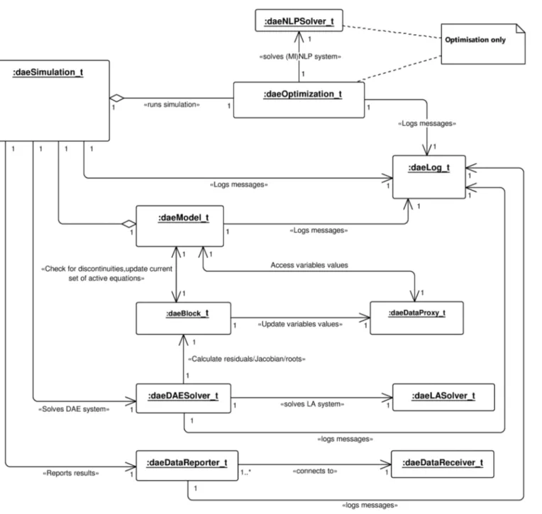
ARCHITECTURE
DAE Tools consists of six packages:core,activity,solvers,datareporting,logging, andunits. All packages provide a set of interfaces (abstract classes) that define the required functionality. Interfaces are realised by the implementation classes. The implementation classes share the same name with the interface they realise with the suffix _tdropped (i.e. the classdaeVariableimplements interfacedaeVariable_t).
Package “core”
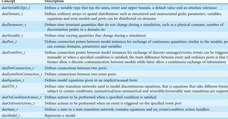
This package contains the key modelling concepts. The class diagram with interfaces (abstract classes) is presented inFig. S1. The most important modelling concepts are given inTable 1. Interface realisations are given inFig. S2. Models in DAE Tools are represented by thedaeModelclass and contain the following elements: domains, parameters, variables, equations, state transition networks, ports, event ports, actions to be performed when a given condition is satisfied, actions to be performed when an event is triggered on a given event port, and components (instances of other models, used to form a hierarchy of models). ThedaeModelUML class diagram is presented inFig. S3.
Package “activity”
Package “solvers”
This package contains interfaces that define an API for numerical solution of systems of Differential Algebraic Equations (DAE), systems of Linear Equations (LA), and (mixed-integer) nonlinear programming problems (NLP or MINLP), and auxiliary classes. The class diagram with the defined interfaces is presented inFig. S4:daeDAESolver_t(defines a functionality for the solution of DAE systems),daeNLPSolver_t(defines a functionality for the solution of (MI)NLP problems),daeLASolver_t(defines functionality for the solution of systems of linear equations) anddaeIDALASolver_t(derived fromdaeLASolver_t,used by Sundials IDAS linear solvers). Interface realizations are given inFig. S5. Current
implementations include Sundials IDAS DAE solver, IPOPT, BONMIN and NLOPT (MI) NLP solvers and SuperLU, SuperLU_MT, PARDISO, Intel PARDISO and Trilinos (Amesos and AztecOO) sparse matrix linear solvers. Since all these linear equation solvers use different sparse matrix representations, a generic interface (templatedaeMatrix<typename FLOAT>) has been developed for the basic operations performed by DAE Tools software such as setting/getting the values and obtaining the matrix properties. This way, DAE Tools objects can access the matrix data in a generic fashion while hiding the internal
implementation details. To date, three matrix types have been implemented:
daeDenseMatrix,daeLapackMatrix(basically wrappers around C/C++ and Fortran two-dimensional arrays), a template classdaeSparseMatrix<typename FLOAT, typename INT> (sparse matrix) and its realizationdaeCSRMatrix<typename FLOAT,typename INT> implementing the Compressed Row Storage (CSR) sparse matrix representation. Table 1 The key modelling concepts in DAE Tools software.
Concept Description
daeVariableType_t Defines a variable type that has the units, lower and upper bounds, a default value and an absolute tolerance
daeDomain_t Defines ordinary arrays or spatial distributions such as structured and unstructured grids; parameters, variables,
equations and even models and ports can be distributed on domains
daeParameter_t Defines time invariant quantities that do not change during a simulation, such as a physical constant, number of
discretisation points in a domain etc.
daeVariable_t Defines time varying quantities that change during a simulation
daePort_t Defines connection points between model instances for exchange of continuous quantities; similar to the models, ports
can contain domains, parameters and variables
daeEventPort_t Defines connection points between model instances for exchange of discrete messages/events; events can be triggered
manually or when a specified condition is satisfied; the main difference between event and ordinary ports is that the former allow a discrete communication between models while latter allow a continuous exchange of information
daePortConnection_t Defines connections between two ports
daeEventPortConnection_t Defines connections between two event ports
daeEquation_t Defines model equations given in an implicit/acausal form
daeSTN_t Defines state transition networks used to model discontinuous equations, that is equations that take different forms
subject to certain conditions; symmetrical/non-symmetrical and reversible/irreversible state transitions are supported
daeOnConditionActions_t Defines actions to be performed when a specified condition is satisfied
daeOnEventActions_t Defines actions to be performed when an event is triggered on the specified event port
daeState_t Defines a state in a state transition network; contains equations and on_event/condition action handlers
Package “datareporting”
This package contains interfaces that define an API for processing of simulation results by thedaeSimulation_tanddaeDAESolver_tclasses, and the data structures available to access those data by the users. Two interfaces are defined:daeDataReporter_t(defines a functionality used by a simulation object to report the simulation results) and daeDataReceiver_t(defines a functionality/data structures for accessing the simulation results). A number of data reporters have been developed for: (a) sending the results via TCP/IP protocol to the DAE Tools Plotter application (daeTCPIPDataReporter), (b) plotting the results using the Matplotlib Python library (daePlotDataReporter), and (c) exporting the results to various file formats (such as MATLAB MAT, Microsoft Excel, html, xml, json and HDF5). An overview of the implemented classes is given inFig. S6.
Package “logging”
This package contains only one interfacedaeLog_tthat define an API for sending messages from the simulation to the user. Interface realizations are given inFig. S7. Three implementations exist:daeStdOutLog(prints messages to the standard output),daFileLog (stores messages to the specified text file), and daeTCPIPLog(sends messages via TCP/IP protocol to thedaeTCPIPLogServer; used when a simulation is running on a remote computer).
Package “units”
Parameters and variables in DAE Tools have a numerical value in terms of a unit of measurement (quantity) and units-consistency of equations and logical conditions is strictly enforced (although it can be switched off, if required). The package contains only two classes:unit andquantity. Both classes have overloaded operators +,-,, / and to
support creation of derived units and operations on quantities that contain a numerical value and units. In addition, the package defines the basic mathematical functions that operate onquantityobjects (such assin,cos,tan,sqrt,pow,log,log10,exp,min,max, floor,ceil,absetc.).
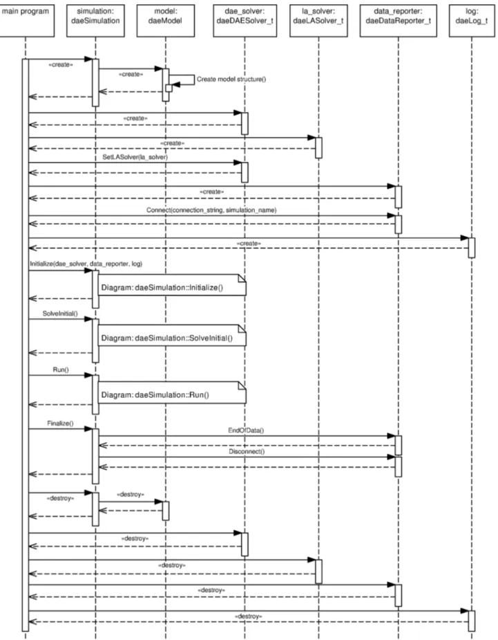
SOLUTION OF A DAE SYSTEM
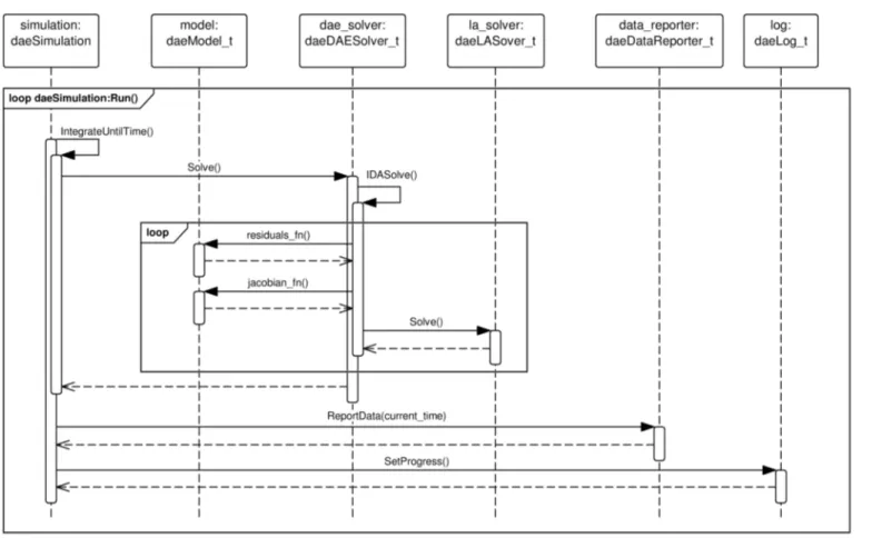
indaeSimulation::SolveInitial()function, (IV) integration of the DAE system in time in daeSimulation::Run()function, and (V) clean-up indaeSimulation::Finalize()function followed by destruction of objects in the main program. A typical sequence of calls during the DAE Tools simulation are given inFig. 2.
Phase I: creation of objects
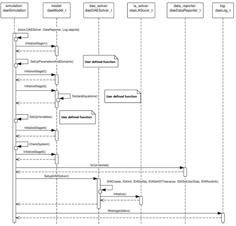
Phase II: initialisation and runtime checks
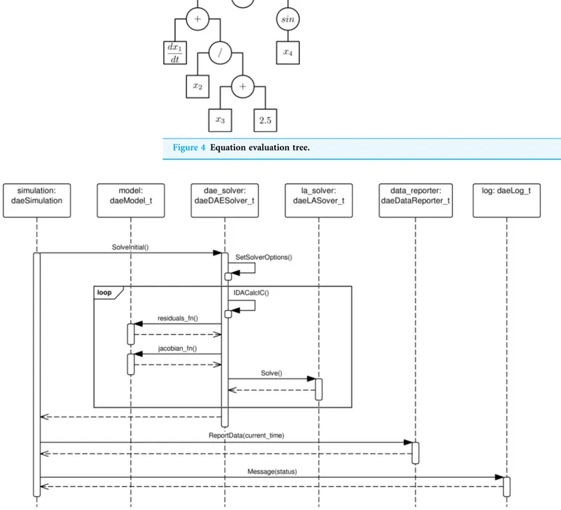
The variables access the data using their global index. The user-defined function SetUpParametersAndDomains() from the daeSimulation-derived class is now called where the parameters values are assigned and the distribution domains initialised. In stage 2 of initialisation, the port and model arrays are created and every variable obtains assigned the global index. Distributed variables obtain a separate index for every point in domains they are distributed on. In stage 3, based on the number of variables and their types, the memory storage for variables values and derivatives is allocated in the data proxy object, the user-defined function DeclareEquations() from the daeModel-derived classes called to create equations, state transition networks, port connections and OnCondition/OnEventhandlers, and the initial variables values and absolute tolerances are set. In the stage 4, the equations get initialised and expanded into an array of residual expressions (one for every point in domains that the equation is distributed on). Every residual expression is evaluated to form an evaluation tree. The concept of representing equations as evaluation trees is employed for evaluation of residual equations and their gradients (which represent a single row in the Jacobian matrix). This is achieved by using the operator overloading technique for automatic differentiation adopted from the ADOL-C library (Walther &
Griewank, 2012). Evaluation trees consist of unary and binary nodes, each node representing a parameter/variable value, basic mathematical operation (+,-,, /,) or
a mathematical function (sin,cos,tan, arcsin, arccos, arctan,sinh,cosh, tanh, arcsinh, arccosh, arctanh, arctan2, erf,sqrt, pow, log,log10, exp,min, max, floor, ceil, abs,sum, product, integral, etc.). The mathematical functions are overloaded to operate on a heavily modified ADOL-C class adouble, which has been extended to contain
information about domains, parameters and variables. In adition, a newadouble_array class has been introduced to support the above-mentioned operations on arrays of parameters and variables. Once built, the evaluation trees can be used for several purposes: (a) to calculate equation residuals, (b) to calculate equation gradients, (c) to export equation expressions into the MathML or LaTeX format, (d) to generate the source code for different languages, and (e) to perform various types of runtime checks. A typical evaluation tree is presented in Fig. 4. In stage 5, the daeBlock instance is created which is used by a DAE solver during the integration of the DAE system. It represents a block of equations and holds the currently active set of equations (including those from state transition networks) and root functions. Finally, the whole system is checked for errors/inconsistencies and the DAE solver initialised.
Phase III: calculation of initial conditions
A sequence of calls during the calculation of initial conditions in daeSimulation:
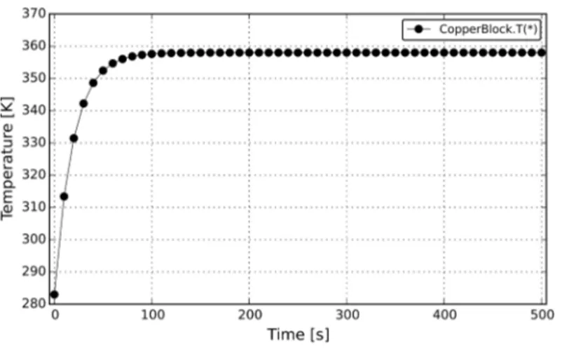
Phase IV: integration in time
A sequence of calls during the integration of the system indaeSimulation::Run()function is given inFig. 6. The default implementation callsdaeSimulation::IntegrateUntilTime() anddaeSimulation::ReportData()functions in a loop until the specified time horizon is
Figure 4 Equation evaluation tree.
reached. TheIntegrateUntilTime()function uses theIDASolve()function that repeatedly calls the functions to evaluate equations residuals, Jacobian matrix and root functions, solves the resulting system of linear equations and checks for possible occurrences of discontinuities until the specified tolerance is achieved.
Phase V: clean up
This phase includes a call todaeSimulation::Finalize()function which performs internal clean-up and memory release, followed by destruction of objects instantiated during phase I.
DEVELOPING MODELS WITH DAE TOOLS
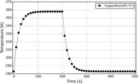
Documentation section of the DAE Toools website (http://www.daetools.com/docs/index. html), subsectionspyDAE User Guide,pyDAE API Reference, andTutorials, respectively. The model describes a block of copper at one side exposed to the source of heat and at the other to the surroundings with the constant temperature and the constant heat transfer
coefficient. The process starts at the temperature of the metal of 283 K. The integral heat balance can be described by the following ordinary differential equation:
mcpdT
dt ¼Qin AðT TsurrÞ
wheremis a mass of the block,cpis the specific heat capacity,Tis the temperature,Qinis the input power of the heater,ais the heat transfer coefficient,Ais the surface area of the block andTsurris the temperature of the surroundings. The copper block model is simulated for 500 s. At a certain point in time, the heat produced by the heater becomes equal to the heat removed by natural convection and the system reaches the steady-state.
Listing 4 CopperBlock model (Python)
fromdaetools.pyDAEimport*
frompyUnitsimportm, kg, s, K, Pa, J, W
# Part 1: creating a model classCopperBlock(daeModel):
def__init__(self, Name, Parent = None, Description =""): daeModel.__init__(self, Name, Parent, Description)
self.m = daeParameter("m", kg, self, "Mass of the copper block") self.cp = daeParameter("c_p", J/(kg*K), self, "Specific heat capacity") self.alpha = daeParameter("α", W/((m**2)*K), self,"Heat transfer coefficient") self.A = daeParameter("A", m**2, self,"Surface area for the heat transfer") self.Tsurr = daeParameter("T_surr", K, self,"Temperature of the surroundings")
self.Qin = daeVariable("Q_in", power_t, self,"Power of the heater") self.T = daeVariable("T", temperature_t, self,"Block temperature")
defDeclareEquations(self):
daeModel.DeclareEquations(self)
eq = self.CreateEquation("HeatBalance","Integral heat balance equation") eq.Residual = self.m() * self.cp() * self.T.dt()-self.Qin() + \
self.alpha() * self.A() * (self.T()-self.Tsurr())
for a specified period of time which is default, or a complex one where various actions can be taken during the simulation). The simulation classes for the copper block model are shown in Source Code Listing 5(Python).
Listing 5 CopperBlock simulation (Python)
# Part 2: setting up a simulation
classsimCopperBlock(daeSimulation):
def__init__(self):
daeSimulation.__init__(self)
self.m = CopperBlock("CopperBlock")
defSetUpParametersAndDomains(self): self.m.cp.SetValue(385 * J/(kg*K)) self.m.m.SetValue(1 * kg)
self.m.alpha.SetValue(200 * W/((m**2)*K)) self.m.A.SetValue(0.1 * m**2)
self.m.Tsurr.SetValue(283 * K)
defSetUpVariables(self):
# Set input power of the heater
# It is a degree of freedom (DOF) and must be assigned
self.m.Qin.AssignValue(1500 * W)
# Set an initial condtion for the temperature
self.m.T.SetInitialCondition(283 * K)
Running a simulation requires the following steps: (a) instantiation of DAE and LA solvers, data reporter, data receiver, and log objects; (b) setting a time horizon and a reporting interval; (c) initialisation of the simulation; (d) calculation of the initial conditions; (e) running simulation; and (f) cleaning up. The simulation performed in Python is given in theSource Code Listing 6. The complete source code of the copper block models developed in Python and C++ are given in theSupplemental Listings S1and S2, respectively. The simulation results for the copper block model are presented inFig. 7.
Listing 6 Running the CopperBlock simulation (Python)
# Part 3: running a simulation
# Create Log, Solver, DataReporter and Simulation object
log = daePythonStdOutLog()
daesolver = daeIDAS()
datareporter = daeTCPIPDataReporter()
simulation = simCopperBlock()
# Enable reporting of all variables
simulation.m.SetReportingOn(True)
# Set the time horizon and the reporting interval
simulation.ReportingInterval = 10
simulation.TimeHorizon = 500
# Connect the TCP/IP data reporter (the default address is "localhost:50000")
datareporter.Connect("","CopperBlock")
# Initialize the simulation
simulation.Initialize(daesolver, datareporter, log)
# Solve the system at time = 0
simulation.SolveInitial()
# Run the simulation
simulation.Run()
# Clean-up
simulation.Finalize()
The previous example was very simple. DAE Tools also support some advanced features such as discontinuous equations and state transition networks. More information about state transition networks and their types can be found in
Barton & Pantelides (1993). Consider a slightly more complex problem now: the same copper block at the ambient temperature (283 K) is allowed to warm up for 200 s, the heat source is then switched off and the metal cools down to the ambient temperature. This problem can be modelled using the concept of symmetrical State Transition Networks (STN); in DAE Tools this type of STN can be created using IF, ELSE_IF, ELSE, and END_IF functions from the daeModel class. From the modellers perspective, these function behave in a similar fashion as ordinary if-else_if-else blocks in all programming languages and select the active set of equations based on the specified logical conditions. The source code of this model is given in Source Code Listing 7 and the simulation results in Fig. 8. The
Listing 7 CopperBlock model with the symmetrical reversible STN (Python)
classCopperBlock(daeModel):
: : :
defDeclareEquations(self):
: : :
self.IF(Time() < Constant(200*s))
eq = self.CreateEquation("Q_on","The heater is on")
eq.Residual = self.Qin()-Constant(1500 * W)
self.ELSE()
eq = self.CreateEquation("Q_off","The heater is off") eq.Residual = self.Qin()
self.END_IF()
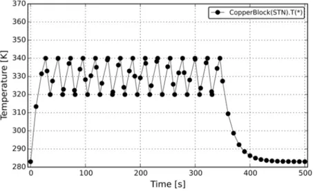
Another commonly used type of state transition networks is a non-symmetrical STN. This type of STN in DAE Tools can be created by using STN, STATE, and END_STNfunctions from thedaeModelclass. To illustrate this concept, consider again the same copper block problem. The process starts again at the temperature of 283 K. However, this time the temperature of the copper block is allowed to reach 340 K and once that is done its temperature is kept in the interval between 320–340 K for 350 s by switching the heater on and off. After 350 s, the heat source
is permanently switched off and the block cools down to the ambient temperature. The source code of the new model is given in Source Code Listing 8 and the simulation results in Fig. 9. The complete source code is given in Supplemental Listing S4.
Listing 8 CopperBlock model with the non-symmetrical irreversible STN (Python)
classCopperBlock(daeModel):
: : :
defDeclareEquations(self):
: : :
self.stnRegulator = self.STN("Regulator")
self.STATE("HeaterOn")
eq = self.CreateEquation("HeaterInput") eq.Residual = self.Qin()- Constant(1500 * W)
self.ON_CONDITION(self.T()> Constant(340*K),
switchToStates = [ (′Regulator′,′HeaterOff′) ] ) self.ON_CONDITION(Time() > Constant(350*s),
switchToStates = [ (′Regulator′,′RegulatorOff′) ] )
self.STATE("HeaterOff")
eq = self.CreateEquation("HeaterInput") eq.Residual = self.Qin()
self.ON_CONDITION(self.T() < Constant(320*K),
switchToStates = [ (′Regulator′,′HeaterOn′) ]) self.ON_CONDITION(Time() > Constant(350*s),
switchToStates = [ (′Regulator′,′RegulatorOff′) ] )
self.STATE("RegulatorOff")
eq = self.CreateEquation("HeaterInput") eq.Residual = self.Qin()
self.END_STN()
APPLICATIONS
To date, DAE Tools have been applied to several diverse scientific areas such as gas adsorption, porous membranes, crystallisation, electrochemistry and biological neural networks. Two projects utilising DAE Tools software at different levels of abstraction are presented in this work. The first example illustrates applicability of DAE Tools to development of multi-scale models. In this example, the authors took advantage of the built-in interoperability with Python NumPy library to perform vector operations on NumPy arrays to form the DAE system. The second example illustrates two important DAE Tools capabilities: (a) embedding into another software (a domain specific language simulator) running on a server and providing its functionality through a web service or web application, and (b) defining the modelling concepts from a new application domain using the DAE Tools fundamental modelling concepts.
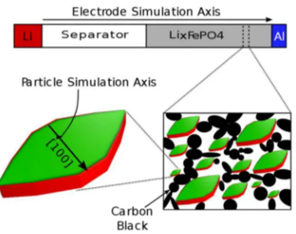
Multi-scale model of phase-separating battery electrodes
Supplemental Information. Spatial discretisation of the governing equations is carried out using the finite volume method, as solid particles are described as residing within individual electrode volumes, as depicted inFig. 10.
The resulting discretised set of equations is a large system of DAE’s. Differential equations come from the discretised transport equations, and algebraic constraints arise from electrostatic equations and constraints on the total integrated reaction rate (current). InLi et al. (2014), the discretised system of DAE’s was integrated in time using MATLAB’s ode15s solver and subsequently reimplemented using DAE Tools, allowing a direct comparison between the two integrators. Using default solver tolerances for both (10-3in MATLAB and 10-5in DAE Tools), a number of simulations were carried out using both the MATLAB implementation and the DAE Tools implementation, and in each case the simulation outputs were indistinguishable. Despite obtaining equivalent outputs, the implementation using DAE Tools consistently ran more quickly (Fig. 11), up to ten times faster (4.22 times, in average). This speedup is a result of its built-in support for automatic differentiation facilitating rapid and accurate derivative evaluation for solution of the highly non-linear system of equations involved in time stepping. In contrast, the ode15s solver creates a numerical approximation of the Jacobian matrix if the Jacobian calculation function is not provided as an input; therefore, the convergence rate is much slower. The significant loss in performance illustrates the benefits of the object-oriented DAE Tools API and the automatic differentiation capabilities it provides, since the calculation of derivatives by hand for all functions in the MATLAB model is very difficult and error-prone for a system of this size and complexity. In addition, the equation-oriented modelling approach made the implementation both easier to code and easier to read in comparison to the non-intuitive mass-matrix approach for coupled differential variables used in the MATLAB version. Finally, the object-oriented approach and clear model separation of DAE Tools also facilitates a much more maintainable and extensible code base in which particle models can be easily interchanged, added, and incorporated into other electrode models.
NineML domain specific language
DAE Tools software has been used as a reference implementation simulator for the “Network Interchange format for NEuroscience” (NineML) Modelling Language. NineML is an open source xml-based domain specific language for modelling of networks of spiking neurones. It is a simulator-independent language with the aim of providing an unambiguous description of neuronal network models for efficient model sharing and reusability between different simulators (such as NEURON, NEST, NeuroML/LEMS etc.). The language has emerged from a joint effort of experts in the fields of computational neuroscience, simulator development and simulator-independent language initiatives (NeuroML, PyNN), grouped in the INCF Multiscale Modelling Task Force (http://www. incf.org). NineML consists of two layers: an Abstraction Layer (AL) contains
and layers; and (d) connectivity patterns–projections, connection probabilities, etc. Apart from the specification, the language contains a set of additional tools: (a) Python library (lib9ml); (b) abstraction layer component tester and report generator (DAE Tools based); and (c) the reference implementation simulator (DAE Tools based). The source code and more information about the language and the whole project can be found on the INCF’s portal (http://software.incf.org/software/nineml).
Abstraction layer component tester and report generator
The purpose of the application is validation and testing of abstraction layer components and generation of model reports (as a help to components developers). The application is available in three flavours: (a) desktop application with the pyQt graphical user interface; (b) web application with the jQuery user interface; and (c) web service with the
REpresentational State Transfer (REST) API. The latter two were implemented using the Web Service Gateway Interface (WSGI) running under Apache HTTP Debian
GNU/Linux server with the mod_python server module. The application inputs are: the AL component, one or more tests (optional), parameters values, initial conditions and inputs to the analogue and event ports. The application produces the model report (in PDF
Figure 11 Parity plot for simulation runs with different inputs (MATLAB vs. DAE Tools).
or html format) and tests results (variable plots). The role of DAE Tools software is to process NineML xml input files, generate the model structure using the lib9ml library, execute the server-side simulations, produce reports and deliver them to the clients.
NineML reference implementation simulator
The NineML reference implementation simulator represents a small scale simulator for testing and validating purposes, with the full support for the NineML language. All input information are given in a simulator-independent format: NineML xml files (mathematical models) and SED-ML xml file (simulation settings). SED-ML is the Simulation Experiment Description Markup Language an xml-based format for encoding simulation experiments (http://sed-ml.org). It is based on the Minimal Information About a Simulation
Experiment guidelines (MIASE,http://biomodels.net/miase) and used to specify: (a) the definition of the model(s) to be used; (b) the definition of the simulation settings to be used; (c) the experimental tasks to be run; and (d) the post processing of the results and outputs (2D-plots, 3D-plots, data tables etc.). The simulator utilises the fundamental modelling concepts in DAE Tools: parameters, variables, equations, ports, models, state transition networks and discrete events as a basis for implementation of the higher-level concepts from the NineML language such as neurons, synapses, connectivity patterns, populations of neurons and projections. Again, the role of DAE Tools software is to process NineML and SED-ML xml input files, generate the model structure, execute the simulation, and produce the results based on inputs from SED-ML file. The simulator implements the synchronous (clock-driven) simulation algorithm and the system of equations is integrated continuously using the variable-step variable-order backward differentiation formula using Sundials IDA DAE solver. The exact event times (spike occurrences) are calculated by detecting
discontinuities in model equations using root functions. An overview of the simulator is presented inFig. 12.
CONCLUSIONS
DAE Tools modelling, simulation and optimisation software, its programming paradigms, the main features and capabilities have been presented in this work. Some shortcomings of the current approaches to mathematical modelling have been recognised and analysed, and a new hybrid approach proposed. The hybrid approach offers some of the key advantages of modelling languages paired with the flexibility of the general purpose languages. Its benefits have been discussed such as the support for the runtime model generation, runtime simulation set-up and complex runtime operating procedures, interoperability with the third party software packages, and embedding and code-generation capabilities. The software architecture and the procedure for transformation of the model hierarchy into a DAE system as well as the algorithm for the solution of the DAE system have been presented. The most important modelling concepts available in the DAE Tools API required for model development and simulation execution have been outlined.
The software has successfully been applied to two different scientific problems. In the first example, the authors took advantage of the object-oriented characteristics of the software and the interoperability with the NumPy library for the development of a model hierarchy to mathematically describe operation of lithium-ion batteries at different physical scales. In the second example, the DAE Tools software has been used as a reference implementation simulator for the new XML-based domain specific language (NineML). DAE Tools embedding capabilities have been utilised to provide a simulator available in three versions: (a) desktop application, (b) web application and (c) web service.
The current work concentrates on a further support for systems with distributed parameters (i.e. high-resolution finite volume schemes with flux limiters), the additional optimisation algorithms and the parallel computation using the general purpose graphics processing units and systems with the distributed memory. The parallel computation will rely on the code generation capabilities to produce the C source code for the DAE/ODE solvers that support the MPI interface such as PETSc and Sundials IDAS/PVODE, including the data partitioning and the routines for the inter-process communication of data.
ACKNOWLEDGEMENTS
The case study Multi-scale model of phase-separating battery electrodeshas been
performed and the corresponding subsection written by Raymond B. Smith, Department of Chemical Engineering, Massachusetts Institute of Technology, Cambridge,
Massachusetts, USA.
ADDITIONAL INFORMATION AND DECLARATIONS
Funding
The author received no funding for this work.
Competing Interests
Author Contributions
Dragan D. Nikolic analyzed the data, wrote the paper, prepared figures and/or tables, performed the computation work, reviewed drafts of the paper.
Data Deposition
The following information was supplied regarding data availability: http://www.daetools.com.
http://sourceforge.net/projects/daetools.
Supplemental Information
Supplemental information for this article can be found online athttp://dx.doi.org/ 10.7717/peerj-cs.54#supplemental-information.
REFERENCES
Akesson J, Arzen K-E, Gafvert M, Bergdahl T, Tummescheit H. 2010.Modeling and optimization with Optimica and JModelica.org–languages and tools for solving large-scale dynamic optimization problems.Computers & Chemical Engineering34(11):1737–1749
DOI 10.1016/j.compchemeng.2009.11.011.
Andersson C, Fuhrer C, Akesson J. 2015.Assimulo: a unified framework for ODE solvers.
Mathematics and Computers in Simulation116:26–43DOI 10.1016/j.matcom.2015.04.007. Balay S, Abhyankar S, Adams MF, Brown J, Brune P, Buschelman K, Dalcin L, Eijkhout V,
Gropp WD, Kaushik D, Knepley MG, McInnes LC, Rupp K, Smith BF, Zampini S, Zhang H. 2015.PETSc users manual. Techical Report ANL-95/11–Revision 3.6, Argonne National Laboratory.Available athttp://www.mcs.anl.gov/petsc/petsc-current/docs/manual.pdf. Barton PI, Pantelides CC. 1993.gPROMS–a combined discrete/continuous modelling
environment for chemical processing systems.Simulation Series25:25–34.
Barton PI, Pantelides CC. 1994.Modeling of combined discrete/continuous processes.AIChE Journal40(6):966–979DOI 10.1002/aic.690400608.
Bonami P, Biegler LT, Conn AR, Cornue´jols G, Grossmann IE, Laird CD, Lee J, Lodi A, Margot F, Sawaya N, Wa¨chter A. 2008.An algorithmic framework for convex mixed integer nonlinear programs.Discrete Optimization5(2):186–204. In Memory of George B. Dantzig
DOI 10.1016/j.disopt.2006.10.011.
Brook A, Kendrick D, Meeraus A. 1988.GAMS, a User’s Guide. SIGNUM Newsletter
23(3–4):10–11DOI 10.1145/58859.58863.
Eaton J, Bateman D, Hauberg S, Wehbring R. 2015.GNU Octave Version 4.0.0 manual: a high-level interactive language for numerical computations.Available at
http://www.gnu.org/software/octave/doc/interpreter/.
Elmqvist H. 1978.A Structured Model Language for Large Continuous Systems. Ph.D. thesis. Lund: Department of Automatic Control, Lund University.
Fritzson P, Aronsson P, Lundvall H, Nystrom K, Pop A, Saldamli L, Broman D. 2005.The openmodelica modeling, simulation, and development environment. In:46th Conference on Simulation and Modelling of the Scandinavian Simulation Society (SIMS2005),Trondheim, Norway, October 13–14, 2005. Oulu: SIMS–Scandinavian Simulation Society.
Fritzson P, Engelson V. 1998.Modelica—a unified object-oriented language for system modeling and simulation. In: Jul E, ed.ECOOP’98—Object-Oriented Programming, Volume 1445 of
Hedengren JD, Shishavan RA, Powell KM, Edgar TF. 2014.Nonlinear modeling, estimation and predictive control in apmonitor.Computers & Chemical Engineering70:133–148 (Manfred Morari Special Issue)DOI 10.1016/j.compchemeng.2014.04.013.
Hindmarsh AC, Brown PN, Grant KE, Lee SL, Serban R, Shumaker DE, Woodward CS. 2005. SUNDIALS: suite of nonlinear and differential/algebraic equation solvers.ACM Transactions on Mathematical Software31(3):363–396DOI 10.1145/1089014.1089020.
Johnson SG. 2015.The NLopt nonlinear-optimization package. Version 2.4.2.Available at
http://ab-initio.mit.edu/wiki/index.php/NLopt.
Li XS. 2005.An overview of SuperLU: algorithms, implementation, and user interface.ACM Transactions on Mathematical Software31(3):302–325DOI 10.1145/1089014.1089017. Li Y, El Gabaly F, Ferguson TR, Smith RB, Bartelt NC, Sugar JD, Fenton KR, Cogswell DA,
Kilcoyne DAL, Tyliszczak T, Bazant MZ, Chueh WC. 2014.Current-induced transition from particle-by-particle to concurrent intercalation in phase-separating battery electrodes.
Nature Materials13(12):1149–1156DOI 10.1038/nmat4084.
MathWorks, Inc. 2015.MATLAB. Matlab 8.5 (R2015a). Natick: MathWorks.Available at
https://mathworks.com/products/matlab.
Morton W. 2003.Equation-oriented simulation and optimization. In:Proceedings of the National Academy of Sciences of India, Section A: Physical Sciences. New Delhi: Springer India3:317–357
Available athttp://www.dli.gov.in/data_copy/upload/INSA/INSA_1/2000c4d6_317.pdf. Piela PC, Epperly TG, Westerberg KM, Westerberg AW. 1991.ASCEND: an object-oriented
computer environment for modeling and analysis: the modeling language.Computers & Chemical Engineering15(1):53–72DOI 10.1016/0098-1354(91)87006-U.
Sala M, Stanley K, Heroux M. 2006.Amesos: a set of general interfaces to sparse direct solver libraries. In:Proceedings of PARA’06 Conference,Umea, Sweden. Available athttps://www. researchgate.net/publication/220840090_Amesos_A_Set_of_General_Interfaces_to_Sparse_ Direct_Solver_Libraries.
Schenk O, Wa¨chter A, Hagemann M. 2007. Matching-based preprocessing algorithms to the solution of saddle-point problems in large-scale nonconvex interior-point optimization.
Computational Optimization and Applications36(2):321–341DOI 10.1007/s10589-006-9003-y. Scilab Enterprises. 2015.Scilab: free and open source software. Version 5.5.2. Versailles: Scilab
Enterprises.Available athttp://www.scilab.org.
Wa¨chter A, Biegler LT. 2006.On the implementation of an interior-point filter line-search algorithm for large-scale nonlinear programming.Mathematical Programming106(1):25–57 DOI 10.1007/s10107-004-0559-y.
Walther A, Griewank A. 2012.Getting started with ADOL-C. Boca Raton: Chapman-Hall CRC Computational Science, 181–202DOI 10.1201/b11644-8.
Waterloo Maple, Inc. 2015.Maple. Waterloo: Waterloo Maple, Inc.Available athttp://www. maplesoft.com/products/maple/.
Wolfram Research, Inc. 2015.Mathematica. Version 10.1. Champaign: Wolfram ResearchInc.